Abstract
With the rapid development of more electric aircraft (MEA) in recent years, the aviation electric power system (AEPS) has played an increasingly important role in safe flight. However, as a highly reliable system, because of its complicated flight conditions and architecture, it often proves significant uncertainty in its failure occurrence and consequence. Thus, more and more stakeholders, e.g., passengers, aviation administration departments, are dissatisfied with the traditional system reliability analysis, in which failure uncertainty is not considered and system reliability probability is a constant value at a given time. To overcome this disadvantage, we propose a new methodology in the AEPS reliability evaluation. First, we perform a random sampling from the probability distributions of components’ failure rates and compute the system reliability at each sample point; after that, we use variance, confidence interval, and probability density function to quantify the uncertainty of system reliability. Finally, we perform the new method on a series–parallel system and an AEPS. The results show that the power supply reliability of AEPS is uncertain and the uncertainty varies with system time even though the uncertainty of each component’s failure is quite small; therefore it is necessary to quantify system uncertainty for safer flight, and our proposed method could be an effective way to accomplish this quantization task.
1. Introduction
Motived by the demand for greener (less gas emission and fuel consumption), more efficient, more flexible, and safer flight, the aircraft industry has seen tremendous progress in the efforts of moving towards more electric aircraft (MEA) [1,2,3]. Compared with conventional aircraft in which on-board loads rely on a combination of pneumatic, mechanical hydraulic, and electrical power, MEA uses electrical power to drive all of these loads [4,5]. As MEA technique develops, aircraft has integrated a large number of electrical loads, many of which are incredibly critical systems for aircraft safety, e.g., flight control system, fuel pumps, and ice-bleeding system [6]. Obviously, the failure of AEPS may cause these critical systems to lose power and consequently lead to severe accidents. For example, on 7 January 2008, a Boeing 747 lost its main power because of water entering the generator control unit and had to use its battery backup. Since this accident happened while the aircraft was descending into Bangkok, there was no serious consequence, but the power loss could cause severe accidents if it took place over the Pacific Ocean [7].
With the goal of decreasing such incidents and accidents, AEPS reliability must be evaluated. Unfortunately, though recently there are many pieces of research about ground power grids [8,9,10,11,12,13], including the mechanism of communication network failure on power system, vulnerability analysis against cyber-attacks, reliability modeling of generation, transmission, and distribution system, etc., they are not suitable for aviation electrical power system (AEPS) as it should be regarded as an irreparable micro-grid during operation with extremely high-reliability requirement which is different from the ground system [14,15]. Up to now, compared with ground power system reliability studies, the literature on AEPS reliability is minimal. Reference [16] proposes a reliability design methodology of three-phase power converters for the applications of aircraft; Reference [17] provides a reliability comparison of various converter topologies. However, these works only analyze the reliability at a component level and the effects of component failure on the entire system not discussed. As a widely used tool in aircraft system reliability analysis, failure mode and effects analysis (FMEA) is always used to investigate the cause-effect relations within the system [18], including the causality between components and the propagation paths from component failure to system failure. Nevertheless, FMEA is only a qualitative method; the quantitative indicators such as system reliability and the mean time to failure (MTTF) of a system cannot be calculated. To perform a quantitative reliability analysis on AEPS at a system level, Reference [6] presents several reliability analysis tools that can be used for AEPS, including Markov analysis, fault tree, and Bayesian network analysis. However, this analysis is in the concept level and no details about system reliability modeling and evaluation. To make these above methods feasible in practice, References [14,19,20,21] put forward practical algorithms for applying minimal cut set, fault tree, minimal path set, and Bayesian network. However, all these works compute system reliability by integrating all the components into an equivalent graph and use constant failure rate for each component without considering the fact that failure rate may vary with loading conditions, weather conditions, pilot experience, etc. This disadvantage in the above works is discussed in Reference [15] and the point of view that component failure rate is an uncertain value rather than a constant value during operation is proposed. However, the uncertainty impacts of the component failure rate on the whole system reliability have not been investigated.
On one hand, it is widely known that AEPS is a large scale system composed of thousands of components, which are provided by thousands of suppliers, as well as a complex network interacting with other aircraft systems such as flight control system and navigation system; Consequently, it is practically impossible for engineers to precisely capture all the characteristics of AEPS, nor understanding the interaction mechanism with other systems completely, which means there must be some epistemic uncertainty [22,23] in AEPS analysis. On the other hand, unlike ground systems, flight environment is exceptionally complicated (aircraft system cannot operate in a static environment); therefore, failure caused by aleatory uncertainty [24] cannot be avoided during flight, either. Accordingly, if the component failure rate is regarded as a constant value, the system reliability must also be a constant probability value, resulting in a loss of the uncertain information mentioned above. However, the uncertainty information is of great importance both for a comprehensive understanding of the system and for the system improvement, such as risk control, maintenance. For instance, to ensure safe flight, the system reliability uncertainty information could be a warning for us that we must take some actions to lower the uncertain risk when the uncertainty information shows that it still has a high potential /probability of falling into an unacceptable low-reliability interval even though the mean value of system reliability is high enough.
Above all, affected by epistemic and aleatory uncertainty, the constant failure rate is just an ideal hypothesis in AEPS reliability analysis, which is not consistent with the truth of practical engineering. In fact, Zio [25,26] proposes that if a system is more natural to be influenced by uncertainties, it is more suitable to treat inner parameters of the system as random variables (however, no details about the reliability evaluation of AEPS in consideration of uncertainty in these works). Inspired by this, to overcome the disadvantages of the existing approaches and to meet the rigid reliability requirement of AEPS, we take the viewpoint that the component’s failure rate in AEPS is a variable which follows some kinds of probability distribution as a starting point and we come up with an approach for AEPS reliability evaluation in the presence of uncertainty. It mainly consists of three steps: first, we use Monte-Carlo simulation method to perform random sampling from the probability distributions of components’ failure rates; and then compute the system reliability (explicitly speaking, system reliability in AEPS refers to the power supply reliability at each load point) at each sample point based on minimal path set method where we obtain the minimal path sets by a combination use of adjacent matrix and depth-first search; thirdly, we obtain the probability density distribution of system reliability as well as the mean value, variance, and confidence intervals of system reliability by managing a statistical calculation on those system reliability values computed in the former step. To verify the proposed approach, we apply this methodology to two examples and give a depth discussion on the effectiveness and reasonability in the aspect of system reliability analysis.
The rest of the paper is organized as follows: Section 2 gives a brief introduction to background of AEPS reliability assessment, including the architecture and function of AEPS, as well as some reliability preliminaries, which is the theoretical basis of the whole paper; Section 3 presents the proposed approach for quantifying how the failure uncertainty in the component level propagates to the uncertainty of system reliability. Section 4, we apply the new method to two systems, one is a series–parallel structure (the basic form of complex AEPS), and the other is a typical AEPS. Conclusions and future work are drawn in Section 5.
2. Background of System Reliability Analysis
2.1. Reliability Preliminaries
Reliability indices: Reliability is defined as the probability of a component to perform its predefined functions under the stated conditions for a given period time [27,28]. The reliability function, R(t) = P(T > t), in practice is usually given by
where N(0) denotes the number of the components at initial time t = 0; N(t) denotes the number of surviving components at time t; F(t) stands for failure function, which is the complementary of reliability function.
Failure rate λ(t) is defined as the probability of the component to fail in the next per unit time, which has not yet failed at time point t. Its observed value is the ration of failures that occurs in t’s next per unit time to the total number of components that still survive at time t, express by
Based on Equation (2), the reliability function R(t) can be written as a function of the failure rate λ(t), expressed as
where the failure rate λ(t) of a component during its life is often described by the Bath-Tub Curve, see Figure 1. It has three periods: early failure period, accidental failure period, and wear out period. In AEPS, components usually operate during the accidental failure period (so this period also called using life), where λ(t) is a constant value λ and Equation (3) is equivalent to
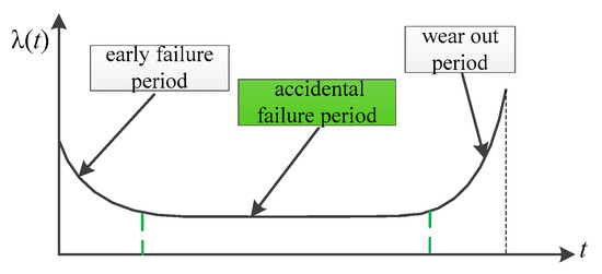
Figure 1.
Bath-Tub Curve [28].
However, it is clear to us that the failure rate is a constant value if and only if the conditions in which the component operates will not change. This is scarcely possible during the flight.
Reliability network: For reliability evaluation, a system is always modeled as a model in which the components are connected in series or parallel. A reliability network is defined as a network structure in which components are connected in a combination of both series and parallel [29], and a typical example of such networks is AEPS.
For a series system, the system operates normally when and only when all the components in this structure work normally, and the system fails as long as one of them fails. According to this logic, the reliability function of a series system composed of N components can be expressed by
For a parallel system, the system fails when and only when all the components in this system fail, and the system can normally work when one of them can operate successfully. According to this logic, the reliability of a parallel system composed of N components can be expressed by
In Equations (5) and (6), represents the reliability function of the system over time under study; Ci represents the ith component of the system; the is the reliability function of the ith component and can be evaluated based on Equation (4) when the failure rate λi of the ith component is known. Please note that we will continue to use these notations N in the following of the paper.
For a reliability network, it is usually hard to extract its equivalent series–parallel form manually, and thus in order to get its reliability function , we need to identify a way to capture all minimal path sets of the network first. A minimal path set is a set of components in which the system can normally work when all the components in the set work successfully, and any failure of them will cause the minimal path set to fail to support the normal work of the system. The system fails when and only when all the minimal path sets fail. Thus, from the point of a functional and logical relationship, all the minimal paths amount to a parallel structure, and components in each minimal path set amount to a series structure, see Figure 2, where the donation represents the ith component of the system’s mth minimal path set, and nm represents the number of components in the mth minimal path set. Then according to Equations (5) and (6), the reliability function of a network can be expressed by
where Ai represents the ith minimal path set of the system; P(Ai) is the work probability of the ith minimal path set and equals to the product of the reliability of components in the ith set; represents the probability that both the ith and jth minimal path work successfully and equals to product of the reliability of components in the ith or jth minimal path set; the notations , and other similar omitted items in Equation (7) have the similar implications with and P(Ai).
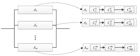
Figure 2.
System equivalent reliability network constructed according to minimal path sets.
2.2. AEPS Reliability Evaluation
A brief introduction to AEPS: An AEPS is designed to deliver power to selected loads. The loads may include avionics, life support, propulsion, communications, guidance, navigation, and control system [6,30]. In general, the primary function of an AEPS is to meet the power requirement of these loads. To achieve this goal, equipment for power generating, power storage, power distribution and operation of loads constitute the architecture of AEPS [31]. A typical AEPS is shown in Figure 3 and more other similar AEPSs with its corresponding introduction can be found in References [1,19,20,21,32,33,34,35].
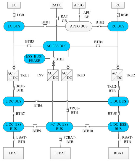
Figure 3.
The architecture of a typical AEPS [21].
In Figure 3, there are four power channel as the power generating consists of four alternators: left and right variable frequency generator (LG, RG), an auxiliary power unit generator (APUG) used as backup when LG and RG fail, and an emergency power unit-ram air turbine generator (RATG) which generates power for essential three-phase alternating current bus (AC ESS BUS) used as backup when LG, RG, and APUG fail. The power storage consists of three main buttery modules: left, right battery (LBAT, RBAT) and flight control battery (FCBATT) which supply direct current (DC) power to left, right essential DC bus (L DC ESS BUS, RDC ESS BUS) and flight control essential DC bus (FC DC ESS BUS). To distribute the energy of power sources generated in battery modules and power generators to the system selected loads which obtain the required power directly from the DC and AC buses (e.g., LG BUS, RG BUS, L DC BUS, etc.), and to prevent over-current from causing unintended damage to the system components, electromechanical current relays, contactors, and breakers are used to route the power from the power sources to the buses by redundancy and reconfiguration. In addition, essential single-phase AC bus (ESS BUS 1 PHASE) is used to support the operation of the single-phase emergency electrical equipment, and a tie bus APUG BUS is used to distributing the power from one channel to other power channels. Finally, one invert (INV) and three transformer rectifier units (TRU) are added to the network at various points for the AC-to-DC and DC-to-AC transfer in the network of AEPS.
AEPS reliability evaluation: Each component such as the generator, battery, transformer rectifier, current relay, bus, etc. can be abstracted as a corresponding node. In particular, the node that corresponds to a generator or battery is defined as a source node, and the node that corresponds to the power supply bus which supports the operation of selected loads is defined as sink node or load point. In addition, if there is power flow from one component to another, then draw a directed line between these two nodes that these two components correspond to. By this definition, the architecture of AEPS can be viewed as a network.
As the function of an AEPS is to deliver the power generated in source nodes to the sink nodes in which the selected loads get the energy they need directly, and there are many sink nodes in one AEPS. In other words, the primary function of an AEPS is equivalent to the statement that whether the required power can be exported from these sink nodes successfully. Thus, unlike traditional system which usually has one probability for quantifying its reliability, AEPS reliability may contain several probabilities, and each refers to the probability of one sink node to perform its intended function of supporting the normal operation of the selected loads, and thus in the following when we say AEPS reliability evaluation, it mean computing the power supply reliability of its each sink node.
In AEPS, we define a sink node’s path set as a way composed of a series of components that can deliver the power generated by a source node to the sink node. Then a minimal path set of one sink node is a way that rules out the repetitive components from its path set. It is clear that we can use Equation (4) and Equation (7) to calculate the exact value of a sink node’s power supply reliability at time t if all the minimal path sets of the sink node and all the components’ constant failure rates are known. Moreover, the sink node’s power supply reliability curve is a linking route of the reliability values at different time t, Figure 4 is an example curve for a sink node’s power supply reliability, where the dot stands for the computed reliability at the selected time point t.
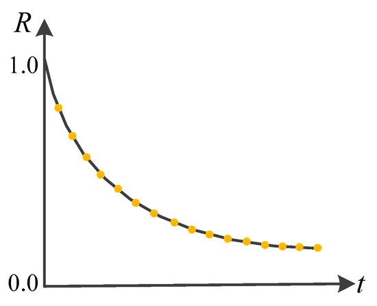
Figure 4.
An example of system reliability curve [32].
3. A Proposed Approach for AEPS Reliability Uncertainty Evaluation
We know that components of AEPS usually operate during their using life period, but we should also know that the failure rate in this period is a roughly average value obtained from multiple data sources by experts or engineers. As the flight conditions change, the failure rate of one component in a different environment must be different. It is not hard to imagine that a component’s failure rate is higher when operating in bad weather than that in good weather, see Figure 5. Moreover, we also know when engineers perform reliability analysis on an AEPS, in traditional method, they should assign each component with a failure rate which is a reference value based on a comprehensive analysis of multiple source data, e.g., laboratory failure data, similar components’ history operating data, data given by component suppliers, etc. However, as AEPS is a complex network of which different engineers have a different understanding, it is scarcely possible for different engineers to reach a consensus on an exact value for each component’s failure rate, in other words, the constant failure rate assigned to each component in practice is an empirical value and the value varies with engineers’ experience, see Figure 6.
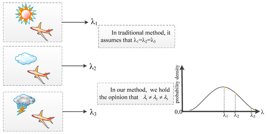
Figure 5.
An example of uncertainty arising from the flight environment.
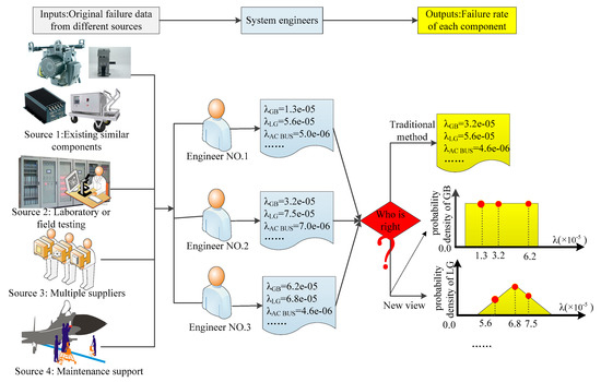
Figure 6.
An example of uncertainty arising from engineer experience.
In the traditional method, the specific value of each component’s failure rate must be decided even though many values for one component are all possible according to current experience and data. By contrast, we hold the view that the values (of course we need rule out the impossible ones first) given by each engineer has its reasonableness and limitations, and thus we depict each component’s failure rate with a probability distribution in which all the possible values given by different engineers can be contained.
Above all, because of the variability of flight environment and the difference of different engineers, there is much uncertainty in components’ failure rates of AEPS. To perform a rigid reliability analysis, it is more suitable for us to treat the component’s failure rate as a random variable that follows some probability distribution [24,26,36,37], such as normal, triangle, and lognormal distribution.
Base on the analysis above, we propose a methodology for AEPS reliability evaluation in the presence of uncertainty. The framework of the proposed system reliability uncertainty analysis in system improvement is provided in Figure 7, and the main steps for system reliability uncertainty calculation are outlined in Figure 8. In the following, we will give a detailed explanation of the proposed method.
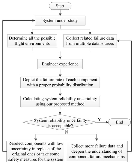
Figure 7.
The framework for system improvement based on system reliability uncertainty analysis.
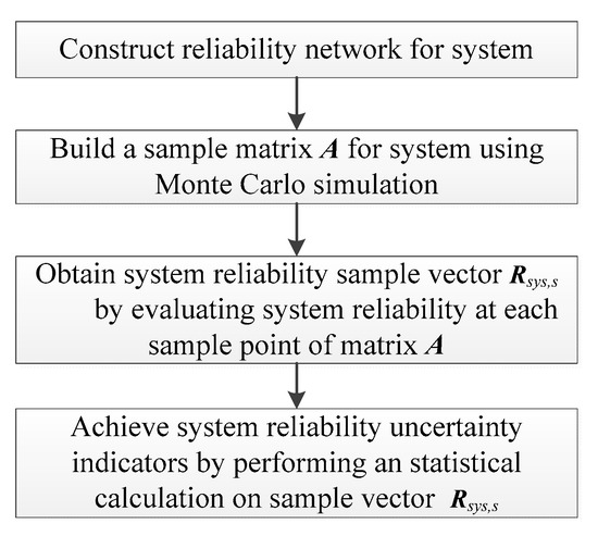
Figure 8.
The flow chart for assessing the reliability uncertainty of AEPS.
① Construct reliability network for system. Here we mean we obtain each sink node’s minimal path sets by performing a depth-first search on the adjacency matrix D of the AEPS, where D is a matrix with dimensions of N × N, and N is the number of components in the AEPS. For the element dij in the matrix D, dij denotes the power direction from node i and node j in the network, and if node i points to node j, then dij = 1, else dij = 0, 1 ≤ i, j ≤ N. By performing a depth-first search on matrix D, we develop an algorithm for obtaining each sink node’s minimal path sets, see Figure 9.
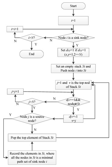
Figure 9.
Algorithm for obtaining minimal path sets by depth-first search.
② Build a sample matrix A for the system. Specifically speaking, for component i (1 ≤ I ≤ N), by using inverse transformation method [38], we generate M pseudo-random numbers λ1i, λ2i…λMi from the probability distribution F(λi) that component i follows. Matrix A composes of these random numbers and expressed by
where the row vector λk of A is the kth sample point of the system, 1 ≤ k ≤ M, and the element λji represents the jth pseudo-random number that we generate from the distribution F(λi). In practice, the probability distribution F(λi) can also be written as its equivalent probability density function form f(λi).
③ Evaluate system reliability at each sample point. To be specific, for k = 1,2…M, we do as follows:
(i) Suppose that the failure rate of the 1st, 2nd … Nth component of the system is equal to the sample value , separately. Based on this, we calculate the reliability of each component by using Equation (4) at a given system time T, and we get a vector .
(ii) As we have got each sink node’s minimal path sets in the first step, the sth sink node’s power supply reliability denoted by can be computed by bringing the parameters into Equation (7), 1 ≤ s ≤ Num, where Num represents the number of sink nodes in AEPS.
The power supply reliability of sink node s at each sample point constitutes a reliability sample vector denoted by .
④ Perform a statistical calculation on sample vector Rsys,s to quantify the uncertainty of system reliability. The quantitative indicators for measuring power supply reliability uncertainty of the sink node s are the sample variance and a (1-α) confidence interval . The mean value is also provided as the auxiliary explanation of these two indicators. The corresponding calculation formula is shown in Equations (9)–(11).
In Equation (11), we generate a new sequence R1, R2…RM by sorting the data of vector Rsys,s according to ascending order, and Rp represents the pth number in the new sequence. Xp represents the confidence limit of vector Rsys,s. We obtain the lower confidence limit by bringing into Equation (11), and obtain the upper confidence limit by setting in Equation (11). When = 0.05, based on Equation (11), we can get a 95% confidence interval of system reliability.
In addition, as the shape of probability density function can reflect the uncertainty level of a system qualitatively, too. In general, the shorter and the fatter the curve of the probability density function of a system is, the more uncertainty it has. Therefore, for an in-depth analysis of the power supply reliability uncertainty of sink node s, we also perform a kernel density function estimation [39] on the sample vector Rsys,s using Equation (12).
Equation (12) is a weighted average, where is the probability density value of power supply reliability of sink node s, h is the bandwidth which can be calculated using the equation based on Rule of Thumb proposed by Silverman [40,41], and the kernel function k(·) is a weight function. As the kernel function is symmetrical about the origin and its integral is 1.0, the Gaussian function can be chosen as the kernel function of Equation (12). Consequently, Equation (12) can be written as Equation (13).
The statement that system reliability uncertainty is acceptable means whether system reliability has an excellent probability of being at a low level, which does not meet the airworthiness regulation or other reliability requirements.
4. Case Study
To illustrate the method, we present two case studies:
1. A system is made up of four components with failure rates lognormally distributed, and we set four sub-cases for this system. In each sub-case, the lognormally distribution parameters are set to be different from the other cases. Then we perform the proposed method to evaluate the system reliability uncertainty in different sub-cases and focus on analyzing the reasonability of the proposed method by a comprehensive comparison of the evaluation results of the four sub-cases.
2. The AC part of the AEPS shown in Figure 3 is discussed, and the failure rates of components are triangle distributed. This case allows us to explain the advantages and the functions of the proposed method, as well as some conclusions about AEPS reliability uncertainty made.
4.1. Reliability Uncertainty Analysis on a Series–Parallel System
Figure 10 is a series–parallel system composed of four components C1, C2, C3, and C4. To verify the new proposed method, four sub-cases that correspond to different uncertainty levels of component’s failure rate are assumed as follows:
| Case 1: | C1: μ1 = −3.5066, σ1 = 0.0; C2: μ2 = −3.5066, σ2 = 0.0; |
| C3: μ3 = −3.5066, σ3 = 0.0; C4: μ4 = −3.5066, σ4 = 0.0; | |
| Case 2: | C1: μ1 = −3.5066, σ1 = 0.05; C2: μ2 = −3.5066, σ2 = 0.05; |
| C3: μ3 = −3.5066, σ3 = 0.05; C4: μ4 = −3.5066, σ4 = 0.05; | |
| Case 3: | C1: μ1 = −3.5066, σ1 = 0.05; C2: μ2 = −3.5066, σ2 = 0.1; |
| C3: μ3 = −3.5066, σ3 = 0.05; C4: μ4 = −3.5066, σ4 = 0.1; | |
| Case 4: | C1: μ1 = −3.5066, σ1 = 0.05; C2: μ2 = −3.5066, σ2 = 0.025; |
| C3: μ3 = −3.5066, σ3 = 0.05; C4: μ4 = −3.5066, σ4 = 0.025. |
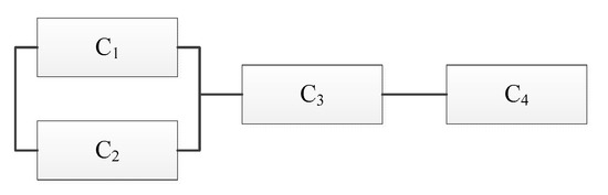
Figure 10.
A series–parallel system.
In the four sub-cases, the failure rate of each component follows a lognormal distribution, see Equation (14), where the standard deviation σi is used to describe the uncertain degree that the failure rate λi varies around the mean failure rate . To discuss the effect of component failure rate uncertainty on system reliability, the mean value μi in each lognormal distribution is set to the same value μi = −3.5066 (the expectation of component failure rate equals to = 0.03), and the standard deviation σi is set to different values in the four sub-cases.
Then we apply the proposed method to the four sub-cases at a given time T = 7 h, the computation results shown in Figure 11 and Table 1. Now we conduct a discussion about the results.
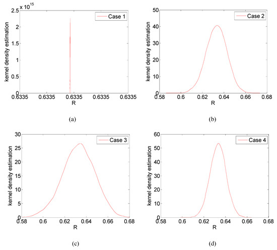
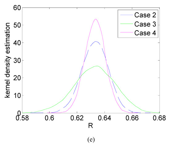
Figure 11.
The kernel density function of the series–parallel system reliability in Case 1~4. (a) Kernel density function in Case 1; (b) Kernel density function in Case 2; (c) Kernel density function in Case 3; (d) Kernel density function in Case 4; (e) System reliability uncertainty comparison of Case 2~4.

Table 1.
The series–parallel system reliability uncertainty results of in Case1~4 (M = 1000).
First, from the second row of Table 1, we see that the mean reliability of the system in four cases basically equals each other. The reason lies in that the mean failure rates of the components under the four cases are the same and equal to 0.03. Theoretically, as the minimal path sets of the system are {C1, C3, C4} and {C2, C3, C4}, based on Equation (7), we can get the theoretical value of the mean reliability of the system by bringing the mean failure rates of components and the minimal path sets into Equation (15).
where R(Ci) = e−0.03T and thus Rsys = 0.633473079. Comparing the theoretical value Rsys with the results obtained using the new method shown in the first row of Table 1, we can see that the absolute errors in the four cases are 0.000027, −0.000273, −0.000773 and −0.000273 separately, and the corresponding relative errors are 0.004%, 0.04%, 0.12%, and 0.04%. It proves that by using our method, the mean reliability of the system can be obtained, or we say that the new method is at least as capable of assessing system reliability as traditional methods.
Secondly, from the second row of Table 1, we see that the variance of Case 1 almost equals 0.0, the variance of Case 2 is slightly more significant than that of Case 4, and Case 3 has a maximum variance among the four cases. The results are in accordance with the 95% confidence interval results of the four cases shown in the third row of Table 1 (the width of 95% confidence interval in Case 1 almost equals to 0.0, the confidence interval in Case 2 is slightly wider than that of Case 4, and the confidence interval in Case 3 is the widest.) Accordingly, the probability density function curve of system reliability in Case 1 obtained by our method is almost an impulse form, the curve of Case 2 is a little shorter and fatter than that of Case 4 and the curve of Case 3 is the “shortest and fattest”, see Figure 11.
All the results stated above indicate that the uncertainty in Case 3 is the largest, Case 2 and Case 4 take the second and third place, separately. There exists no uncertainty for the system in Case 1.
To illustrate the correctness of the results we get, we turn back to look at the standard deviation σi we assigned to the four sub-cases. It can be seen that the standard deviation σi of each failure rate in Case 1 is set to 0.0, which means no uncertainty existing in component failure or we say each failure rate is a constant value in Case 1; and thus theoretically, the system reliability must be a specific value on the basis of Equations (4) and (15), which is in accordance with the result that no uncertainty exists in Case 1 we computed. Moreover, it is clear that the standard deviation σi of the same component in Case 3 is either equivalent to or larger than that of the other cases; therefore, the system reliability in Case 3 has the most massive uncertainty. In addition, because the standard deviation σi of C2 and C4 in Case 2 is more significant than those in Case 4, system reliability uncertainty in Case 2 is more significant than that in Case 4.
Based on the analysis above, we conclude that the uncertainty of system reliability caused by component failure uncertainty can be adequately evaluated by using our proposed simulation method, and at a given time T the more uncertainty that the component has, the more uncertain the system reliability is.
It is important to note that although the results we compute are at an assumed time T = 7 h, using the proposed method, we can also get similar uncertainty results at other assumed system time T, i.e., the parameter T does not affect the above conclusions, we are free to assume a different time T and apply the proposed method to the four cases.
4.2. Reliability Uncertainty Analysis of Aviation Electric Power System
In this part, we apply the new method to analyze the AC subsystem of Figure 3, the components which contain are LG, LGB, LG BUS, BTB1, APUG BUS, APU GB, APUG, BTB2, RG BUS, RGB, RG, BTB3, AC ESS BUS, BTB4, RATG, RATGB, BTB5, INV, and ESS BUS 1 PHASE. There are four sink nodes (power supply buses) supporting the operation of AC electrical equipment in the system, and they are LG BUS, RG BUS, AC ESS BUS, and ESS BUS 1 PHASE. With regard to component failure rate in aircraft engineering, it is often shown that different experts or engineers have a consensus on the order of magnitude that one component’s failure rate should be approximately within by taking the general changes in flight conditions (e.g., climate, weather, and flight load) into consideration, but it is difficult to reach a consensus on the specific value that the component’s failure rate should exactly be because of the difference of different personal experience. In addition, hence, when we refer to different papers (see References [14,15,20,21,32,34]), we see that even for the same component, different values of the failure rate are provided in different papers while these values are all almost in the same order of magnitude, i.e., if one component’s failure rate is 5.00 × 10⁻⁶ per hour in some literature, in fact, the failure rate have a tremendous potential probability of being a value that ranges from 1.00 × 10⁻⁶ to 9.99 × 10⁻⁶ per hour (when considering some more extreme or complex flight condition than usual, or estimating failure rate by less experienced engineers, the failure rate can also change beyond its generic orders of magnitude, here we do not consider this extreme condition. In other words, the uncertainty that we assign to the component of AEPS is much conservative here), and 5.00 × 10⁻⁶ per hour just may be the most likely value of the failure rate according to the available data and generic personal experience. Triangle distribution is useful in depicting a random variable if one only knows the maximum, minimum, and the most likely value of it, and thus here we treat each failure rate λi as a variable that obeys such a distribution shown in Equation (16), where the mode λmode is the value that is repeated most often in the Reference [14,21], the upper limit λupper and lower limit λlower of the triangle distribution is the maximum and minimum value among the numbers of the same order of magnitude with the mode value λmode, see Table 2.
Table 2.
Component failure rates of AC subsystem.
We set system time T = 1000 h, T = 2000 h…T = 60,000 h, and apply the new method to compute power supply reliability of the sink node LG BUS, RG BUS, AC ESS BUS, and ESS BUS 1 PHASE. The minimal path sets of each sink node obtained by the algorithm in Figure 9 are listed in Table A1 in Appendix A; the achieved power supply reliability of LG BUS and RG BUS at these time points is shown in Table 3, as well as that of AC ESS BUS and ESS BUS 1 PHASE shown in Table 4. Moreover, the corresponding kernel density function curve of power supply reliability of LG BUS at T = 5000 h, T = 10,000 h, T = 15,000 h, T = 20,000 h, and T = 250,000 h, is provided in Figure 12; the variance curve of power supply reliability of each sink node over system time T is also presented in Figure 13. Now we perform an in-depth analysis on these results.
Table 3.
Power supply reliability uncertainty results of LG BUS and RG BUS (M = 10,000).
Table 4.
Power supply reliability uncertainty results of AC ESS BUS and ESS BUS 1 PHASE (M = 10,000).
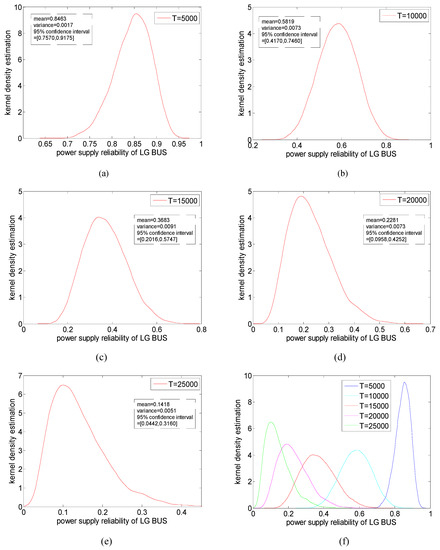
Figure 12.
The kernel density function of LG BUS power supply reliability at different time T. (a) Kernel density function at T = 5000; (b) Kernel density function at T = 10,000; (c) Kernel density function at T = 15,000; (d) Kernel density function at T = 20,000; (e) Kernel density function at T = 25,000; (f) Comparison of kernel density function at different T.
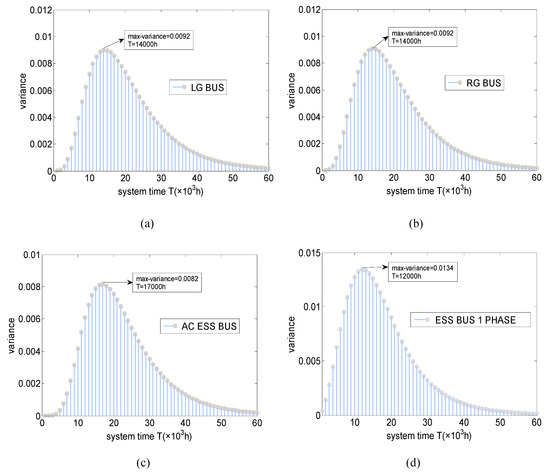
Figure 13.
Power supply reliability variance of each sink node over system time T. (a) Power supply reliability variance of LG BUS; (b) Power supply reliability variance of RG BUS; (c) Power supply reliability variance of AC ESS BUS; (d) Power supply reliability variance of ESS BUS1 PHASE.
First, in comparison with the traditional reliability results of Table A2 in Appendix A in which each sink node’s power supply reliability is a constant value at a given system time T and none uncertainty information is revealed in the final result, according to the results in Table 3 and Table 4 achieved by the new method, it is no doubt that the power supply reliability of each sink node shows an apparent uncertainty even though the failure uncertainty of each component is quite small (Both the maximum and minimum possible failure rate of each component is in the same order of magnitude); i.e., our method can quantify the reliability uncertainty of AEPS effectively. For example, we see that for the power supply reliability of LG BUS, its mean reliability is 0.9896, and 95% confidence interval is [0.9831, 0.9947] at T = 1000 h. That means the reliability has a probability of 0.95 varying from 0.9831 to 0.9947 (the width of confidence interval is 0.0116), and for safety-critical system, it is a degree of uncertainty which cannot be neglected; as is known that from the point of safety control and maintenance, system reliability being 0.98 is very different from system reliability being 0.99 for strict airworthiness regulations. Usually, to improve system reliability by 10 × 10−5, much effort and money would be cost (e.g., carefully redesign and evaluation by more experienced experts, choose some more reliable and expensive component, strong maintenance support). In addition, for passengers, the intuitive feelings of safety under these two values are also very different, for example, when one passenger knows the system reliability is 0.9947 after a just 1000 h of continuous system operation without any maintenance, he will take the airplane with a high probability and else if he knows the reliability also may be 0.9831 which is below 0.99, he may give up on the airplane. On the other hand, we find that LG BUS power supply reliability gotten in the traditional method is a constant value 0.9935. It is just one possible value in the interval [0.9831, 0.9947] we computed, and it proves to be more optimistic than the uncertainty reliability results as it is a high percentile in the interval and is larger than the mean value 0.9896 of uncertainty results. In addition, from Figure 12c, we even see that LG BUS power supply reliability still has a potential of being larger than 0.6 after a continuous operation of 15,000 h without any maintenance, but it also has a potential of being less than 0.2; furthermore, by comparing the reliability results for LG BUS in Table 3 and Table A2 at T = 15,000 h, we find the power supply reliability in traditional method is still far more optimistic than the uncertainty results. All the data proves that even though failure uncertainty of all the components is not apparent, they may also cause very significant uncertainty for the power supply reliability of LG BUS as system time increases. For other sink nodes, similar comparison results can also be obtained. Overall, the uncertainty information of power supply reliability missed in traditional results can be captured using our method, which cannot only helps engineers decide when measures should be taken to improve the system as Figure 7 but also helps other stakeholders, e.g., passengers, aviation administration departments, gain a more comprehensive understanding of system reliability and make more reliable decisions.
Secondly, we see that the uncertainty of the power supply reliability of each sink node is time-varying even though the parameter of the probability distribution each component’s failure rate obeys is constant. To be specific, according to the obtained variance each sink node’s power supply reliability in Table 3 and Table 4, we note that the uncertainty increases with time at first, then it reaches a peak value at some system time point, finally, it decreases from the peak. Accordingly, from Figure 12, we can find that the kernel density function curve of power supply reliability of LG BUS at T = 15,000 h is the shortest and fattest among the curves at T = 5000 h, T = 10,000 h…T = 25,000 h, which proves that the power supply reliability uncertainty of LG BUS is a parabolic function of system time when the component failure rate distribution is given, which can also be demonstrated in Figure 13a. In addition to LG BUS, according to the variance curves in Figure 13b–d, we can also see that the uncertainty of power supply reliability of RG BUS, AC ESS BUS, and ESS BUS 1 PHASE shows the same changing rule with system time T.
Why does system reliability uncertainty change with system time T, and is the changing rule we achieved that system reliability uncertainty is a parabolic function of system time T reasonable? Generally speaking, according to Equation (4), each component’s failure probability is quite small at the initial operation stage of system (T equals a small value), and thus the system inevitably runs safely and reliably with a high probability, which necessarily leads to a small uncertainty for system reliability at such an early stage. We can explain it in an extreme way, suppose that the system time T is 0 now, on the base of Equation (7) it is not difficult for us to imagine that the system is bound to run successfully (system reliability is 1.0) no matter whether the component failure rate is constant or not because each component must be reliable at T = 0 on the basis of Equation (4), which means there is no uncertainty, or we say reliability uncertainty is 0 at T = 0 because system success is a deterministic event at this time.
As T advances, the system reliability is undoubtedly a process of gradual decrease from 1.0. The system reliability is no longer 1.0 and begins to show some uncertainty because the uncertainty of component failure rate begins to have an effect on the whole system when T does not equal to 0 according to Equations (4) and (7). Due to the non-negative nature of uncertainty, the system reliability uncertainty must increase from its initial value 0 as system reliability uncertainty gradually appears from T = 0.
Moreover, when T increases to a time point at which the chance for system failure is approximately equivalent to the chance for system operating successfully, because it is a most challenging time to figure out the system is successful or in fail, the system reliability uncertainty inevitably reaches its peak at such a time point. To illustrate this, taking LG BUS power supply reliability as example, from Table 3 and Figure 12, we know that when system time is around T = 10,000~15,000 h, the 95% confidence interval has a high potential of including the reliability value of 0.5, indicating that the probability of system being successful and that of being in fail is basically equivalent during T = 10,000~15,000 h; then we turn to the variance values at these time points in Table 3 and Figure 13a, we can find that the uncertainty of LG BUS power supply reliability reaches its peak around system time T = 14,000 h, belonging to the time interval 10,000~15,000 h.
As T increases further from the peak time point, the chance for system failure increases and begins to be higher than that for system operating successfully, which means that compared with peak time point, it begins to become more accessible for us to distinguish the system state (successful or in fail), and hence system uncertainty begins to decrease. We can explain it in another extreme way when T increase to positive infinity, the reliability of each component must be 0 on the base of Equation (4), therefore system reliability must tend to be 0.0 according to Equation (7); i.e., the system state is a deterministic failure event when T = +∞, hence the uncertainty of system reliability inevitably equals 0 again.
All in all, from the changing process of system reliability with system time T explained above, we can conclude that system reliability uncertainty is a changing process that when T changes from 0, it increases from 0, and reaches to the peak around the time point when the chance for system failure is approximately equivalent to that for system operation, and then it decreases from the peak when T increases further, finally, it goes back to be 0 when T tends to infinity. Clearly, the process explained above is in accordance with the results we have achieved that power supply reliability uncertainty is a quadratic function of system time T with a maximum value.
In the AC subsystem of Figure 3, Generator includes LG, APUG, RG, RATG; AC BUS includes LG BUS, RG BUS, APUG BUS, AC ESS BUS, ESS BUS 1 PHASE; BTB/GB includes LGB, RGB, APUGB, BTB1~BTB4.
5. Conclusions and Future Work
As the traditional method for system reliability analysis cannot capture the uncertainty at a system level which caused by epistemic and aleatory uncertainty, we are committed to finding a method for quantifying and computing the system reliability uncertainty that propagates from component failure uncertainty. First, we briefly summarize the AEPS architecture and its reliability calculation method under the assumption that the failure rate of each component is a constant value; Furthermore, based on the Monte-Carlo simulation principle, in consideration of failure rate uncertainty, we put forward the probability density function, variance, and confidence interval of the system reliability as the indicators for measuring system reliability uncertainty, as well as the method for computing these indicators are presented and explained in detail. The main contribution of our work can be summarized as follows: (1) To the author’s knowledge, it is the first work in the literature to propose a method for assessing AEPS system reliability in consideration of failure uncertainty. Unlike traditional methods using constant component failure rate, the impact of component failure uncertainty on the whole system reliability is quantified in our work. (2) The reliability evaluation of two systems is performed by the newly proposed method, which proves the validity of the method. The results of the first system show that our proposed method has the ability of depicting system reliability uncertainty effectively under different level of component failure uncertainty; the results of the second system, a real-world AEPS, show that system reliability uncertainty is a quadratic function of system time T, and the uncertainty (measured by variance, confidence interval, and the probability density function) of system reliability may be significant and we must pay attention to it even though the component failure has a low degree of uncertainty.
Though it proves that the new method can provide theoretical reference for the AEPS reliability uncertainty analysis, but the following limitations still exist: (1) In the example of the aviation power system in our paper, the probability distribution of the failure rate of each component is based on the existing literature and expert experience, not directly calculated from historical data. Therefore, in the following, we will focus on the calculation of the probability distribution of the component failure rate on the base of the existing failure data. (2) We know during the flight, AEPS should be regarded as an irreparable micro-grid, which is very different from the ground system, but it does not mean AEPS cannot be maintained daily. In fact, the daily maintenance quality always has a significant impact on the system reliability, for example, good/lousy maintenance can improve/decreases reliability. In this paper, this maintenance has not been considered so far, which is more complicated than the usual ground system. Hence, how to integrate the maintenance factor into the reliability uncertainty analysis is another research direction.
Author Contributions
Conceptualization, Y.W. and X.G.; Funding acquisition, M.Y.; Investigation, Y.C.; Methodology, Y.W.; Project administration, S.L.; Resources, M.Y.; Software, Y.W. and Y.C.; Supervision, Y.L.; Validation, Y.W. and S.L.; Writing—original draft, Y.W.; Writing—review and editing, X.G. All authors have read and agreed to the published version of the manuscript.
Funding
The research was funded by the Natural Science Foundation of Shaanxi Provincial Department of Education of 2018 (No. 18JK0572) and Foundation item: Quality and Reliability Fundamental Project of China’s Ministry of Industry and Information Technology’s Twelfth Five-year Plan (No. 2052013B003).
Conflicts of Interest
The authors declare no conflict of interest.
Appendix A
Table A1.
Minimal path sets of AC subsystem.
Table A1.
Minimal path sets of AC subsystem.
| Sink Node | List | The Components of Each Minimal Path Set in AC Subsystem |
|---|---|---|
| LGBUS | 1 | LGBUS, LGB, LG |
| 2 | APUG, APUGB, APUG BUS, BTB1, LG BUS | |
| 3 | RG, RGB, RG BUS, BTB2, APUG BUS, BTB1, LG BUS | |
| RGBUS | 1 | RG, RG, RG BUS |
| 2 | APUG, APUGB, APUG BUS, BTB2, RG BUS | |
| 3 | LG, LGB, LG BUS, BTB1, APUG BUS, BTB2, RG BUS | |
| AC ESS BUS | 1 | LG, LGB, LG BUS, BTB3, AC ESS BUS |
| 2 | APUG, APUGB, APUG BUS, BTB1, LG BUS, BTB3, AC ESS BUS | |
| 3 | RG, RGB, RG BUS, BTB2, APUG BUS, BTB1, LG BUS, BTB3, AC ESS BUS | |
| 4 | RG, RGB, RG BUS, BTB4, AC ESS BUS | |
| 5 | APUG, APUGB, APUG BUS, BTB2, RG BUS, BTB4, AC ESS BUS | |
| 6 | LG, LGB, LG BUS, BTB1, APUG BUS, BTB2, RG BUS, BTB4, AC ESS BUS | |
| 7 | RATG, RATGB, AC ESS BUS | |
| ESS BUS 1 PHASE | 1 | LG, LGB, LG BUS, BTB3, AC ESS BUS, BTB5, ESS BUS 1 PHASE |
| 2 | APUG, APUGB, APUG BUS, BTB1, LG BUS, BTB3, AC ESS BUS, BTB5, ESS BUS 1 PHASE | |
| 3 | RG, RGB, RG BUS, BTB2, APUG BUS, BTB1, LG BUS, BTB3, AC ESS BUS, BTB5, ESS BUS1PHASE | |
| 4 | RG, RGB, RG BUS, BTB4, AC ESS BUS, BTB5, ESS BUS 1 PHASE | |
| 5 | APUG, APUGB, APUG BUS, BTB2, RG BUS, BTB4, AC ESS BUS, BTB5, ESS BUS 1 PHASE | |
| 6 | LG, LGB, LG BUS, BTB1, APUG BUS, BTB2, RG BUS, BTB4, AC ESS BUS, BTB5, ESS BUS1PHASE | |
| 7 | RATG, RATGB, AC ESS BUS, BTB5, ESS BUS 1 PHASE | |
| 8 | FCBAT, FC DC ESS BUS, INV, BTB5, ESS BUS 1 PHASE |
Table A2.
Power supply reliability of four sink nodes by using the traditional method of Section 2.2.
Table A2.
Power supply reliability of four sink nodes by using the traditional method of Section 2.2.
| T (h) | LG BUS | RG BUS | AC ESS BUS | ESS BUS 1 PHASE |
|---|---|---|---|---|
| 1000 | 0.9935 | 0.9935 | 0.9950 | 0.9814 |
| 2000 | 0.9829 | 0.9829 | 0.9895 | 0.9624 |
| 3000 | 0.9678 | 0.9678 | 0.9830 | 0.9427 |
| … | … | … | … | … |
| 11,000 | 0.7200 | 0.7200 | 0.8369 | 0.7334 |
| 12,000 | 0.6821 | 0.6821 | 0.8066 | 0.6998 |
| 13,000 | 0.6443 | 0.6443 | 0.7747 | 0.6651 |
| 14,000 | 0.6071 | 0.6071 | 0.7414 | 0.6299 |
| 15,000 | 0.5708 | 0.5708 | 0.7073 | 0.5944 |
| 16,000 | 0.5355 | 0.5355 | 0.6727 | 0.5590 |
| 17,000 | 0.5014 | 0.5014 | 0.6379 | 0.5239 |
| 18,000 | 0.4687 | 0.4687 | 0.6033 | 0.4896 |
| 19,000 | 0.4375 | 0.4375 | 0.5692 | 0.4561 |
| … | … | … | … | … |
| 59,000 | 0.0185 | 0.0185 | 0.0244 | 0.0098 |
| 60,000 | 0.0170 | 0.0170 | 0.0225 | 0.0089 |
References
- Roboam, X. New trends and challenges of electrical networks embedded in “more electrical aircraft”. In Proceedings of the 2011 IEEE International Symposium on Industrial Electronics, Gdansk, Poland, 27–30 June 2011; pp. 26–31. [Google Scholar]
- Buticchi, G.; Costa, L.; Liserre, M. Improving system efficiency for the more electric aircraft: A look at dc\/dc converters for the avionic onboard dc microgrid. IEEE Ind. Electron. Mag. 2017, 11, 26–36. [Google Scholar] [CrossRef]
- Sarlioglu, B.; Morris, C.T. More electric aircraft: Review, challenges, and opportunities for commercial transport aircraft. IEEE Trans. Transp. Electrif. 2015, 1, 54–64. [Google Scholar] [CrossRef]
- Rosero, J.A.; Ortega, J.A.; Aldabas, E.; Romeral, L. Moving towards a more electric aircraft. IEEE Aerosp. Electron. Syst. Mag. 2007, 22, 3–9. [Google Scholar] [CrossRef]
- Van Den Bossche, D. The A380 flight control electrohydrostatic actuators, achievements and lessons learnt. In Proceedings of the 25th International Congress of the Aeronautical Sciences, Hamburg, Germany, 3–8 September 2006; pp. 1–8. [Google Scholar]
- Telford, R.D.; Galloway, S.J.; Burt, G.M. Evaluating the reliability & availability of more-electric aircraft power systems. In Proceedings of the 2012 47th International Universities Power Engineering Conference (UPEC), London, UK, 4–7 September 2012; pp. 1–6. [Google Scholar]
- Knox, W.B.; Mengshoel, O. Diagnosis and reconfiguration using Bayesian networks: An electrical power system case study. In Proceedings of the 21st International Joint Conference on Artificial Intelligence, Pasadena, CA, USA, 13–17 July 2009; pp. 67–74. [Google Scholar]
- Shuvro, R.A.; Wang, Z.; Das, P.; Naeini, M.R.; Hayat, M.M. Modeling impact of communication network failures on power grid reliability. In Proceedings of the 2017 North American Power Symposium (NAPS), Morgantown, WV, USA, 17–19 September 2017; pp. 1–6. [Google Scholar]
- Jin, M.; Lavaei, J.; Johansson, K.H. Power grid ac-based state estimation: Vulnerability analysis against cyber attacks. IEEE Trans. Autom. Control 2018, 64, 1784–1799. [Google Scholar] [CrossRef]
- Kakran, S.; Chanana, S. Smart operations of smart grids integrated with distributed generation: A review. Renew. Sustain. Energy Rev. 2018, 81, 524–535. [Google Scholar] [CrossRef]
- Cadini, F.; Agliardi, G.L.; Zio, E. A modeling and simulation framework for the reliability/availability assessment of a power transmission grid subject to cascading failures under extreme weather conditions. Appl. Energy 2017, 185, 267–279. [Google Scholar] [CrossRef]
- Rosas-Casals, M.; Valverde, S.; Solé, R. A simple spatiotemporal evolution model of a transmission power grid. IEEE Syst. J. 2018, 12, 3747–3754. [Google Scholar] [CrossRef]
- Cortes, C.A.; Contreras, S.F.; Shahidehpour, M. Microgrid topology planning for enhancing the reliability of active distribution networks. IEEE Trans. Smart Grid 2017, 9, 6369–6377. [Google Scholar] [CrossRef]
- Zhao, Y.; Che, Y.; Lin, T.; Wang, C.; Liu, J.; Xu, J.; Zhou, J. Minimal Cut Sets-Based Reliability Evaluation of the More Electric Aircraft Power System. Math. Problems Eng. 2018, 2018, 1–11. [Google Scholar] [CrossRef]
- Xu, Q.; Xu, Y.; Tu, P.; Zhao, T.; Wang, P. Systematic Reliability Modeling and Evaluation for On-Board Power Systems of More Electric Aircrafts. IEEE Trans. Power Syst. 2019, 34, 3264–3273. [Google Scholar] [CrossRef]
- Burgos, R.; Chen, G.; Wang, F.; Boroyevich, D.; Odendaal, W.G.; Van Wyk, J.D. Reliability-oriented design of three-phase power converters for aircraft applications. IEEE Trans. Aerosp. Electron. Syst. 2012, 48, 1249–1263. [Google Scholar] [CrossRef]
- Aten, M.; Towers, G.; Whitley, C.; Wheeler, P.; Clare, J.; Bradley, K. Reliability comparison of matrix and other converter topologies. IEEE Trans. Aerosp. Electron. Syst. 2006, 42, 867–875. [Google Scholar] [CrossRef]
- Kritzinger, D. Aircraft System Safety: Military and Civil Aeronautical Application; Woodhead Publishing: Cambridge, UK, 2006. [Google Scholar]
- Zhang, B. Applying Reliability Analysis to Design Electric Power Systems for More-Electric Aircraft. Ph.D. Thesis, Graduate School, University of Maryland, College Park, MD, USA, 2014. [Google Scholar]
- Chwa, J.; Ameri, A.; Mozumdar, M. Improving reliability of aircraft electric power distribution system. In Proceedings of the 2014 IEEE Green Energy and Systems Conference (IGESC), Long Beach, CA, USA, 24–24 November 2014; pp. 61–66. [Google Scholar]
- Wang, Y.; Yang, M.; Miao, Z.; Dong, X. A Reliability Modelling Method for Aircraft Electrical Power System Based on Probability Network. In Proceedings of the 2018 5th International Conference on Mathematics and Computers in Sciences and Industry (MCSI), Corfu, Greece, 25–27 August 2018; pp. 155–159. [Google Scholar]
- Xiahou, T.; Liu, Y.; Jiang, T. Extended composite importance measures for multi-state systems with epistemic uncertainty of state assignment. Mech. Syst. Signal Proc. 2018, 109, 305–329. [Google Scholar] [CrossRef]
- Ferson, S.; Joslyn, C.A.; Helton, J.C.; Oberkampf, W.L.; Sentz, K. Summary from the epistemic uncertainty workshop: Consensus amid diversity. Reliab. Eng. Syst. Saf. 2004, 85, 355–369. [Google Scholar] [CrossRef]
- Crespo, L.G.; Kenny, S.P.; Giesy, D.P. Reliability analysis in the presence of Aleatory uncertainty. In Safety and Reliability–Safe Societies in a Changing World; CRC Press: Boca Raton, FL, USA, 2018; pp. 2349–2357. [Google Scholar]
- Zio, E. The Monte Carlo Simulation Method for System Reliability and Risk Analysis; Springer: London, UK, 2013. [Google Scholar]
- Baraldi, P.; Zio, E.; Compare, M. A method for ranking components importance in presence of epistemic uncertainties. J. Loss Prev. Process Ind. 2009, 22, 582–592. [Google Scholar] [CrossRef]
- Modarres, M.; Kaminskiy, M.P.; Krivtsov, V. Reliability Engineering and Risk Analysis: A Practical Guide, 3rd ed.; CRC Press: Boca Raton, FL, USA, 2016. [Google Scholar]
- Elsayed, E.A. Reliability Engineering, 2nd ed.; John Wiley & Sons: Hoboken, NJ, USA, 2012; pp. 1–120. [Google Scholar]
- Fotuhi-Firuzabad, M.; Billinton, R.; Munian, T.S.; Vinayagam, B. A novel approach to determine minimal tie-sets of complex network. IEEE Trans. Reliab. 2004, 53, 61–70. [Google Scholar] [CrossRef]
- Mengshoel, O.J.; Chavira, M.; Cascio, K.; Poll, S.; Darwiche, A.; Uckun, S. Probabilistic model-based diagnosis: An electrical power system case study. IEEE Ttans. Syst. Man. Cybern. A 2010, 40, 874–885. [Google Scholar] [CrossRef]
- Poll, S.; Patterson-Hine, A.; Camisa, J.; Garcia, D.; Hall, D.; Lee, C.; Sweet, A. Advanced diagnostics and prognostics testbed. In Proceedings of the 18th International Workshop on Principles of Diagnosis (DX-07), Nashville, TN, USA, 29–31 May 2007; pp. 178–185. [Google Scholar]
- Cai, L.; Zhang, L.; Yang, S.; Wang, L. Reliability assessment and analysis of large aircraft power distribution systems. Acta Aeronaut. Astronaut. Sin. 2011, 32, 1488–1496. [Google Scholar]
- Tang, B.; Yang, S.; Wang, L.; Zhang, H. Commercial aircraft distribution network reconfiguration based on power priority. In Proceedings of the 2016 IEEE 2nd Annual Southern Power Electronics Conference (SPEC), Auckland, New Zealand, 5–8 December 2016; pp. 1–5. [Google Scholar]
- Zhang, Y.; Kurtoglu, T.; Tumer, I.Y.; O’Halloran, B. System-Level Reliability Analysis for Conceptual Design of Electrical Power Systems. In Proceedings of the Conference on Systems Engineering Research (CSER), Redondo Beach, CA, USA, 14–16 April 2011; pp. 15–16. [Google Scholar]
- Bozhko, S.V.; Wu, T.; Hill, C.I.; Asher, G.M. Accelerated simulation of complex aircraft electrical power system under normal and faulty operational scenarios. In Proceedings of the IECON 2010 36th Annual Conference on IEEE Industrial Electronics Society, Glendale, AZ, USA, 7–10 November 2010; pp. 333–338. [Google Scholar]
- Zafiropoulos, E.P.; Dialynas, E.N. Reliability and cost optimization of electronic devices considering the component failure rate uncertainty. Reliab. Eng. Syst. Saf. 2004, 84, 271–284. [Google Scholar] [CrossRef]
- Blanks, H.S. Arrhenius and the temperature dependence of non-constant failure rate. Qual. Reliab. Eng. Int. 1990, 6, 259–265. [Google Scholar] [CrossRef]
- Kroese, D.P.; Taimre, T.; Botev, Z.I. Handbook of Monte Carlo Methods; John Wiley & Sons: Hoboken, NJ, USA, 2013; pp. 43–85. [Google Scholar]
- Scaillet, O. Density estimation using inverse and reciprocal inverse Gaussian kernels. J Nonparametr. Stat. 2004, 16, 217–226. [Google Scholar] [CrossRef]
- Silverman, B.W. Density Estimation for Statistics and Data Analysis; CRC Press: Baca Raton, FL, USA, 1986; pp. 34–75. [Google Scholar]
- Bianchi, M. Bandwidth selection in density estimation. In Xplore: An Interactive Statistical Computing Environment; Springer: New York, NY, USA, 1995; pp. 101–112. [Google Scholar]
© 2020 by the authors. Licensee MDPI, Basel, Switzerland. This article is an open access article distributed under the terms and conditions of the Creative Commons Attribution (CC BY) license (http://creativecommons.org/licenses/by/4.0/).