Novel Mode Adaptive Artificial Neural Network for Dynamic Learning: Application in Renewable Energy Sources Power Generation Prediction

Abstract

A reasonable dataset, which is an essential factor of renewable energy forecasting model development, sometimes is not directly available. Waiting for a substantial amount of training data creates a delay for a model to participate in the electricity market. Also, inappropriate selection of dataset size may lead to inaccurate modeling. Besides, in a multivariate environment, the impact of different variables on the output is often neglected or not adequately addressed. Therefore, in this work, a novel Mode Adaptive Artificial Neural Network (MAANN) algorithm has been proposed using Spearman’s rank-order correlation, Artificial Neural Network (ANN), and population-based algorithms for the dynamic learning of renewable energy sources power generation forecasting model. The proposed algorithm has been trained and compared with three population-based algorithms: Advanced Particle Swarm Optimization (APSO), Jaya Algorithm, and Fine-Tuning Metaheuristic Algorithm (FTMA). Also, the gradient descent algorithm is considered as a base case for comparing with the population-based algorithms. The proposed algorithm has been applied in predicting the power output of a Solar Photovoltaic (PV) and Wind Turbine Energy System (WTES). Using the proposed methodology with FTMA, the error was reduced by 71.261% and 80.514% compared to the conventional fixed-sized dataset gradient descent-based training approach for Solar PV and WTES, respectively.

1. Introduction

The application of Machine Learning (ML) has broken the barrier of correctly predicting different physical systems. The application of ML can be found in all sorts of industries. In today’s world, renewable energy-based sources are an integrated part of almost any power system. The successful prediction of renewable energy sources is highly essential for successful electricity market participation. These sources are highly weather-dependent; therefore, predicting the plant output is a challenging task. The research and application of ML for renewable energy sources plant output prediction has been increased in recent years. The increase in the number of publications indirectly indicates the necessity of such research, development in the ML field, and improved computational capacities. In Section 1.1 and Section 1.2, a brief discussion on the reviewed literature is conducted, where the necessity and scope for more research on this field can be found. The actual and abbreviated forms of the technical terms found in the reviewed literature and used in this paper are listed in

Table 1. List of abbreviations/acronyms found in reviewed literature and used in this work.

Full-Form	Abbreviation	Full-Form	Abbreviation
Mode Adaptive Artificial Neural Network	MAANN	Stationary Wavelet Transform	SWT
Artificial Neural Network	ANN	Random Forest	RF
Advanced Particle Swarm Optimization	APSO	Machine Learning and Statistical Hybrid Model	MLSHM
Fine-Tuning Metaheuristic Algorithm	FTMA	Auto-Gate Recurrent Unit	Auto-GRU
Photovoltaic	PV	Deep Learning	DL
Wind Turbine Energy System	WTES	Genetic Algorithm-based ANN	GA-ANN
Machine Learning	ML	Radiation Classification Coordinate	RCC
Feedforward Backpropagation	FFBP	Recurrent Neural Network	RNN
Feedforward Neural Network	FFNN	Conjugated Gradient Neural Network	CGNN
Multilayer Feed-Forward with Backpropagation Neural Networks	MFFNNBP	Neuro-Fuzzy System with Grid Partition	NF-GP
Nonlinear Autoregressive Network with Exogenous Inputs-based Neural Network	NARXNN	Enhanced PSO	EPSO
Bayesian Regularization	BR	Deep Neural Network-based Meta-Regression and Transfer learning	DNN-MRT
Levenberg-Marquardt	LM	Principal Component Analysis	PCA
Deep Belief Network	DBN	Gradient Boosting Tree	GBT
Long Short-Term Memory	LSTM	Least Absolute Shrinkage Selector Operator	LASSO
Adaptive Neuro-Fuzzy Inference System	ANFIS	k Nearest Neighbor	kNN
Adaptive Backpropagation	ABP	Extreme Gradient Boost	xGBoost
General Regression Neural Network	GRNN	Artificial Intelligence and Numerical Weather Prediction	AI-NWP
Backpropagation Neural Network	BPNN	Multiple Linear Regression	MLR
Elman Neural Network	ENN	Neuro-Fuzzy system with Subtractive Clustering	NF-SC
Multi-Layer Perceptron	MLP	Least-Square Support Vector Regression	LSSVR
Particle Swarm Optimization	PSO	M5 Regression Tree	M5RT
Particle Swarm Optimization-based Artificial Neural Network	PSO-ANN	Support Vector Machine	SVM
Broyden-Fletcher-Goldfarb-Shanno Quasi-Newton	BFGSQN	Correlation Coefficient	CC
Resilient Backpropagation	RB	Autoregressive Integrated Moving Average with Explanatory Variable	ARIMAX
Linear Regression	LR	Mean Squared Error	MSE
Support Vector Regression	SVR	Bayesian Information Criterion	BIC
Random Tree	RT	Mean Absolute Error	MAE
M5P Decision Tree	M5PDT	Standard Deviation of the Errors	SDE
Gaussian Process Regression	GPR	Sum of Squared Errors	SSE
Physical Photovoltaic Forecasting Model	P-PVFM	Gradient Descent	GD
Distributed Extreme Learning Machine	DELM	Decision Tree	DT

.

1.1. Literature Review for Output Power Prediction of Solar Photovoltaic (PV) System

Reviewed literature for solar PV systems can be broadly categorized according to the application of the variants of the neural network and hybrid methods. Under the category of variants of the neural network, different models such as Feedforward Backpropagation (FFBP), Feedforward Neural Network (FFNN), Multilayer Feed-Forward with Backpropagation Neural Networks (MFFNNBP), etc., with different learning algorithms, namely, Bayesian Regularization (BR) and Levenberg-Marquardt (LM), can be found in References [1,2,3,4,5,6,7,8,9]. In this category, the application of advanced neural network models, that is, Deep Belief Network (DBN), Autoencoder [10], Long Short-Term Memory (LSTM) [10,11,12], and Adaptive Neuro-Fuzzy Inference System (ANFIS) [13], was also found. In Reference [14], Adaptive Backpropagation (ABP) is used for dynamic training of the network. In the mentioned works, the proposed methods were compared with many neural network-based models. For example, General Regression Neural Network (GRNN) [1], Backpropagation Neural Network (BPNN), Elman Neural Network (ENN) [8], Multi-Layer Perceptron (MLP) [10,12], etc., with different training algorithms, for instance, PSO-ANN [13], LM [4,6], BR, Broyden-Fletcher-Goldfarb-Shanno Quasi-Newton (BFGSQN), Resilient Backpropagation (RB), etc. [6]. Also, many non-neural network-based methods have been applied for comparisons. Linear Regression (LR) [2,7], persistent [2], Support Vector Regression (SVR), Random Tree (RT) [5], M5P Decision Tree (M5PDT), Gaussian Process Regression (GPR) [7], and Physical Photovoltaic Forecasting Model (P-PVFM) [10] are some examples of such methods.

Under the category of hybrid methods, Distributed Extreme Learning Machine (DELM), and an information fusion rule-based hybrid model, have been found in Reference [15]. Similarly, other hybrid methods such as ANN-PSO with K-mean clustering [16], Stationary Wavelet Transform (SWT) with Random Forest (RF) [17], ML, image processing, and acoustic classification-based technique [18] are also found. Machine Learning and Statistical Hybrid Model (MLSHM) and Auto-GRU are found in Reference [19]. Authors have proposed a generalized ensemble model integrating Deep Learning (DL) techniques for solar power forecasting in Reference [20]. Additionally, a separate ensemble algorithm was assigned for clustering the dataset. The GA-ANN method for solar power forecasting was proposed in Reference [21]. Finally, in Reference [22], a simple Radiation Classification Coordinate (RCC)-LSTM-based algorithm for very short-term solar power forecasting was proposed, where the proposed model has achieved better accuracy over other compared models.

1.2. Literature Review for Output Power Prediction of Wind Turbine Energy System (WTES)

In the case of WTES, the reviewed literature can be broadly classified into three categories. Category one is the variants of neural networks, where the application of probabilistic neural network with Recurrent Neural Network (RNN) [23], DBN [24], Conjugated Gradient Neural Network (CGNN) [25], RNN [26], and Neuro-Fuzzy System with Grid Partition (NF-GP) [27] can be found. Hybrid models of neural network class such as SVR with Enhanced PSO (EPSO)-ANN [28], Deep Neural Network-based Meta-Regression and Transfer learning (DNN-MRT) [29], hybrid model using Principal Component Analysis (PCA) and DL [30], hybrid LSTM [31], and LSTM-RNN [32] are also found. Non-neural network-based ML algorithms, namely, CART-Bagging [33], Gradient Boosting Tree (GBT) [34], Least Absolute Shrinkage Selector Operator (LASSO), k Nearest Neighbor (kNN), Extreme Gradient Boost (xGBoost), RF and SVR [35], Artificial Intelligence and Numerical Weather Prediction (AI-NWP) [36], Decision Tree (DT), and RF [37] are found, too. The mentioned methodologies are mostly compared with Multiple Linear Regression (MLR) [28], persistence approach [34], Neuro-Fuzzy system with Subtractive Clustering (NF-SC), Least-Square Support Vector Regression (LSSVR), M5 Regression Tree (M5RT) [27], and Support Vector Machine (SVM) [37], etc.

1.3. Research Gaps and Motivation for the Proposed Methodology

The reviewed works have demonstrated the supremacy of ML/DL, and almost all the papers have given importance to the size of the dataset, forecasting duration, forecasting methodology, model performance, etc. But two important factors, which are dynamic learning (except References [14,17] for solar PV and Reference [34] for WTES), and determination of output impacting dominant input variables, also known as correlation analysis (except References [2,6,16,20,22] for solar PV and Reference [32] for WTES) were not covered. Also, none of them were applied together. The necessity of dynamic learning and correlation analysis is discussed in Section 1.3.1 and Section 1.3.2. The discussed works are summarized in

Table 2. Summary of the reviewed literature.

Solar PV
Category	Proposed Methodology	Compared Methodologies	Correlation Analysis	Dynamic Learning
Variants of neural network	ANN (FFBP/FFNN/MFFNNBP/NARXNN) [1,2,3,4,5,6,7,8,9] DBN [10], Autoencoder [11], LSTM [10,11,12], ANFIS [13], ABP [14]	GRNN [1], LR [2,7], persistent [2], LM [4,6], SVR, RT [5], BR, BFGSQN, RB etc. [6], M5PDT, GPR [7], BPNN, BPNN-GA, ENN, etc. [8], MLP [8,10], P-PVFM [10], SVM [12], PSO-ANN [13]	Yes [2,6]	Yes [14]
Hybrid Models	ANN-PSO with K-mean clustering [16], DELM and information fusion rule combined [15], SWT and RF combined [17], ML, Image Processing, and acoustic classification-based technique [18], MLSHM and Auto-GRU [19], General ensemble model with DL technique [20], GA-ANN [21], RCC-LSTM [22]	SVR [16], LSTM [22]	Yes [16,20,22]	Yes [17]
Wind Turbine Energy Systems
Category	Proposed Methodology	Compared Methodologies	Correlation Analysis	Dynamic Learning
Variants of neural network	Probabilistic neural network with RNN [23], DBN [24], CGNN [25], RNN [26], NF-GP [27]	NF-SC, LSSVR, M5RT [27]	Not found	Not found
Hybrid Models	SVR and Hybrid SVR with EPSO-ANN [28], DNN-MRT [29], PCA and DL [30], Hybrid LSTM [31], LSTM-RNN [32]	MLR [28], Four multivariate model [31]	Yes [32]	Not found
Non-neural network ML	CART-Bagging [33], GBT [34], ML [35], AI-NWP [36], DT, and RF [37]	Persistence approach [34], LASSO, kNN, xGBoost, RF and SVR [35], SVM [37]	Not found	Yes [34]

, featuring different categories, proposed, and compared methodologies, correlation analysis, and dynamic learning.

1.3.1. Necessity of Dynamic/Online Learning

Dynamic learning, which is commonly known as online learning, overcomes the problem of model training with a big fixed-sized dataset. The use of gradient descent backpropagation for neural network-based model training requires data division into multiple batches, as single batch training using all the samples in the training set may not guarantee an optimal model. On the other hand, dynamic learning trains the system with each entry of the data from the environment. An optimized model from the previous data entry can be a near-optimal solution point for the current data entry, making learning/training faster. The necessity of dynamic learning for renewable energy sources can be understood from Figure 1 and the related explanation.

If the model is trained using a “small” sized dataset, although the error of the model can be well below the acceptable error limit (black straight line), as the new data enters the system, due to lack of training on similar data, the error of the model may surpass the acceptable limit. Thus, in the future, a loss in profit may incur due to suboptimal performance. On the other hand, if a “big” sized dataset is chosen, the participant will lose its profit during the (Big-Critical) sized dataset duration by not participating in the market, as the model already reached its optimal state after the critical point (in terms of error performance). A dynamic learning approach can be adopted to participate in the market if the model error goes below the acceptable error limit. The model can stop participating, then retrain, and re-participate if the error gets larger. The conceptual diagram of the dynamic learning procedure can be understood from Figure 2.

As per the conceptual diagram, the forecasting model goes under the training/optimization cycle to reduce the error between the actual output from the physical system and predicted output from the forecasting model. The condition for training, training algorithms, etc., can be included inside the ’Forecasting model optimization’ block. This block considers all the previous data entries for optimization, as consideration of the current state will produce an optimal model for current input data only, which will fail to perform efficiently in the presence of different data, or data similar to previous/historical entries.

1.3.2. Necessity of Correlation Coefficient (CC) Analysis among the Input and Output Variables

Considering too many variables to develop a forecasting model increases the complexity. Also, all the variables may not have a dominant impact on the output. CC calculation can be a useful tool for determining dominant input variables. Application of Pearson correlation coefficient [38] analysis or sensitivity analysis on a fixed dataset was found in the literature as a CC analysis tool. Pearson correlation coefficient analysis works fine when a linear relationship between the considered variables (input and output) exists. Also, due to dependency on the data sample size, the use of CC analysis on a fixed-sized dataset may not represent the actual or stable relationship between the variables (input and output). To overcome the problem of dynamical selection of dominant variables, applications of tensor-based [39], autoregressive [40], and embedding-based methods [41] are found in a few recent studies. The applications are useful for multi-plant forecasting and change detection from multivariate time-series data from the smart grid considering the online/dynamic learning with smaller feature space. However, the use of Autoencoder [41] with a neural network-based forecasting model increases the complexity, as two different models (Autoencoder for feature extraction and neural network for forecasting) need to train on such a case. Also, Autoencoder does not guarantee the extracted features’ orthogonality; therefore, collinearity issues may exist in the reduced feature space [41]. The use of tucker decomposition in the tensor-based method has limitations with rank estimation, and the stability of the proposed method needs to confirm with different rank values [39]. Although these methods are beneficial, there always remains some scope to work with different algorithms that are yet to be implemented and can be used effectively.

1.4. Contribution of This Research

Therefore, considering the discussed problems, in this work, a dynamic learning algorithm has been proposed to train a variable structured ANN, which changes according to the selected dominant input variables. Each combination of the input variables is defined as “Mode.” Thus, the proposed algorithm has been named as “Mode Adaptive Artificial Neural Network (MAANN).” This adaptation of the Modes is made through dynamic CC analysis using Spearman’s rank-order correlation [42] algorithm. Spearman’s rank-order correlation algorithm performs robustly for both linear and nonlinear variables. Dynamic use of this algorithm helps the operator to choose dominant input variables and reveals the stability of the relationship between the variables. A stable relationship can be used to find the optimal size of the dataset or training termination criteria.

Also, in contrast to the conventional gradient descent and Autoregressive Integrated Moving Average with Explanatory Variable (ARIMAX) training technique, in this work, dynamic learning methodology has been proposed using some recent metaheuristic algorithms. Metaheuristic algorithms overcome the premature convergence and local minimum trapping problem of the gradient descent algorithm. Also, metaheuristic algorithms iteratively improve the result using the population set. Additionally, in this work, to avoid premature convergence, modification in the population-based algorithms has also been introduced, which is described in Section 2.

Therefore, the contributions of the work can be summarized as follows:

i.

Determination of dominant input variables and data stability analysis using the dynamic application of Spearman’s rank-order correlation.

ii.

Application of recent population-based algorithms for better accuracy of the forecasting models compared to the conventional approach (fixed-sized dataset training with gradient descent and ARIMAX algorithm).

iii.

Algorithm validation by application on two different types of renewable sources of different locations, with different numbers of input variables and dataset size.

The paper has been organized as follows: in Section 2, related theories for the proposed algorithm are discussed. The selection of the dominant input variables and dataset stability determination using the Spearman rank-order correlation is also discussed in Section 2. In Section 3, the flow chart of the proposed algorithm is presented in detail. Section 4 consists of a description of the sites and the dataset, experimental results discussion, and analysis. Finally, in Section 5, the conclusion and scopes for the future works are presented. Before explaining the major sections, the list of the symbols frequently used in this article has been listed and shown in

Table 3. List of symbols used in this work.

Symbol	Description	Symbol	Description
$n$	Number of input variables	$p_g^b$	Best remembered swarm positions
$N$	Number of hidden layer nodes	$W_{max}$ and $W_{min}$	Maximum and Minimum value of inertia
$\mathrm{f}$	Output function of the single-layer feedforward neural network	$Max gen$	Maximum number of generations
$OW$	Output layer weight vector $\in R^{1xN}$	$\mathrm{pop}$	Size of the population for the metaheuristic optimizations
$\xi (.)$	Hidden layer activation function	$p$ and $r$	Random variables associated with the FTMA exploitation and randomization stage
$IW$	Input layer weight matrix$\in R^{Nxn}$	$\rho$	Spearman’s rank-order correlation
$y$	Arbitrary input variable	$d$	Rank wise distance between two variables
$OB$	Bias of the output layer	$th$	Correlation coefficient Threshold value
$j$	Input variable sample number	z	Predefined number of sample entry when ANN training can be stopped
$l$	Number of observations/lengths of the input variables	$eph$	Error threshold limit for training
$\widehat{Y}$ and $Y$	predicted and actual output of the ANN	$Z^{\prime }$	Min–Max feature scaling variable
$x$	solution particle	$X_{max}$, $X_{min}$	Minimum and Maximum value of the input variable
$i$	Location/position of any arbitrary solution from the set of the solution vector	$Y_{max}, Y_{min}$	Minimum and Maximum value of the output variable
$k$	any parameter (weights/biases) within the neural network which needs to be optimized	$m$	Arbitrary occurrence number of a specific Mode
$g$	Generation number	M	Mode number
$rand$	Random number (ranges within 0–1)	$k^{\prime }$	Number of parameters to be estimated
$v$	Velocity of the solution particle	$\widehat{L}$	Maximized value of the likelihood function of the Model
$w$	Inertia (ranges within 0–1)	P	Number of parameters (weights and biases) in ANN in case of BIC
$c_1$ and $c_2$	Cognitive and social parameters(range between 0 and 2)	$\sigma$	Standard deviation
$p_g^i$	Best remembered individual position	$\mu$	Mean of the population

.

It should be mentioned that the solution particle $x$ changes with the change in the optimization iteration cycle. Therefore, the changed values of solution positions are mentioned using the super and subscripts, which can be found in the descriptions of the optimization algorithms of Section 2.2.

2. Related Theories for the Proposed Methodology

ANN, metaheuristic algorithms, and Spearman’s rank-order correlation are the heart of the proposed dynamic learning algorithm. Therefore, in this section, an introduction to the concepts are given.

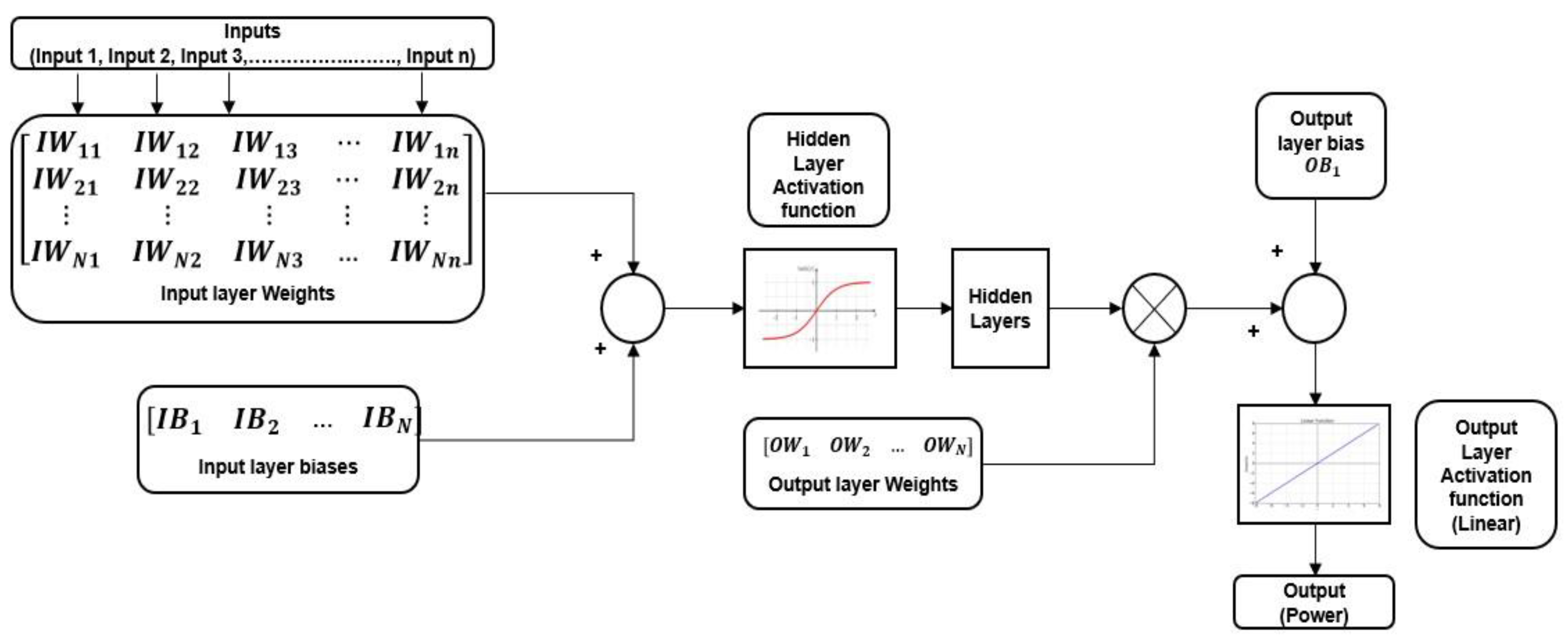
2.1. Artificial Neural Network (ANN)

Among the different ANN structures found in many studies in the literature, feedforward neural network [1,3,14] has been used in this work. The internal weights and biases will be varied according to the choice of input variables by correlation analysis. Figure 3 shows the ANN model in a vector-matrix notational-based structure.

The following equation can describe the output of a single layer feed forward neural network:

$$\mathrm{f}\left(y_j\right)=OW.\xi \left(IW.y_j+IB\right)+OB, j=1,\dots \dots \dots ,l$$

(1)

where $y_j$ is the $j^{th}$ sample input of the input variable $y$. The hyperbolic tangent function has been used as the hidden layer activation function in this work [43]. In the output layer, a linear activation function is used. Once the neural network’s predicted output is calculated using Equation (1), next, the error between the actual and predicted output should be calculated. In this work, to calculate the error during the learning process, Mean Squared Error ($\mathrm{MSE}$) is considered:

$$\mathrm{MSE}=\underset{\left(IW,IB,OW,OB\right)}{argmin}\frac{1}{l}{\displaystyle \sum }_{j=1}^l{\left({\widehat{Y\left(IW,IB,OW,OB\right)}}_j-Y_j\right)}^2$$

(2)

where, ${\widehat{Y}}_j \mathrm{and} Y_j$ are the predicted and actual output of the $j^{th}$ sample respectively, and $l$ is the number of training samples. The objective is to find the optimal values of weights $\left\{IW, OW\right\}$, and biases $\left\{IB,OB\right\}$, such that the error is reduced.

2.2. Optimization Algorithms

As discussed earlier, in this work, metaheuristic algorithms are used for the optimization (commonly known as training of ANN) of MAANN. Metaheuristic algorithms are population-based algorithms, and many of them are characterized by exploration and exploitation features. The exploration and exploitation feature improves optimization performance. The definition of exploration and exploitation properties can be found in Reference [44]. A general-purpose universal optimization strategy is impossible according to the No Free Lunch theory [45]; hence, there is always some scope to improve the result using new optimization techniques. Thus, three recent algorithms with fewer hyperparameters were chosen in this work. The chosen algorithms are: Jaya Algorithm (2016, hyperparameter: 0), Advanced Particle Swarm Optimization (APSO) (2018, hyperparameter: 3), and Fine-Tuning Metaheuristic Algorithm (FTMA) (2019, hyperparameter: 2).

2.2.1. Description of Jaya Algorithm

Jaya algorithm was proposed by Rao in 2015 [46]. It is a gradient-free algorithm and does not contain any hyperparameter. The essence of the Jaya algorithm is the Equation (3):

$$x_{k,\mathrm{i},g+1}=x_{k,\mathrm{i},\mathrm{g}}+rand\left(x_{k,best,\mathrm{g}}-\left|x_{k,\mathrm{i},\mathrm{g}}\right|\right)-rand\left(x_{k,worst,\mathrm{g}}-\left|x_{k,\mathrm{i},\mathrm{g}}\right|\right)$$

(3)

where $x_{k,i,g}$ is the $i^{th}$ candidate’s value of the $k^{th}$ variable at the $g^{th}$ iteration, $x_{k,best,g}$ and $x_{k,worst,g}$ are the best and worst values of the $k^{th}$ variable at the $g^{th}$ iteration, and $x_{k,i,g+1}$ is the updated position/value of the candidate solution.

2.2.2. Description of APSO

PSO [47] is a population-based stochastic optimization technique developed by Eberhart and Kennedy in 1995, whereas APSO was proposed in 2018 by Khan et al. [48]. The velocity and position updating equations of APSO are shown in Equations (4) and (5), respectively. Inertia, $w,$ in Equation (4) can be controlled according to Equation (6):

$$v_{g+1}^i=w{v}_g^i+c_{1}rand\left(p_g^i-x_g^i\right)+c_{2}rand\left(p_g^b-x_g^i\right)+w\left(\frac{c_1}{c_2}\right)\left(p_g^i-p_g^b\right)$$

(4)

$$x_{g+1}^i=x_g^i+v_{g+1}^i$$

(5)

$$w_g=W_{max}-\frac{\left(W_{max}-W_{min}\right)\left(g-1\right)}{Max gen}$$

(6)

The original velocity equation of PSO is modified by adding a third term on the right-hand side of Equation (4). The additional term is used to minimize the particles’ positions iteratively by increasing the velocity to reach the optimal solution faster [48]. In Equations (4) and (5), $x_g^i$,$v_g^i$, and $x_{g+1}^i$,$v_{g+1}^i$ are the $i^{th}$ particle positions and velocities in the $g^{th}$ and $g+1^{th}$ generations. A description of the remaining variables can be found in Table 3.

2.2.3. Description of FTMA

FTMA was proposed by Allawi et al. in 2019 [49] to solve global optimization problems. The fundamental equations describing the algorithm that is exploration, exploitation, and randomization are shown in Equations (7)–(9):

$$x_{exploration}\left(k\right)=x_i^g\left(k\right)+rand\left(x_j^g\left(k\right)-x_i^g\left(k\right)\right), i=1,2,\dots \dots \dots , \mathrm{pop} and i\ne j$$

(7)

$$x_{exploitation}\left(k\right)=x_i^g\left(k\right)+rand\left(x_{best}^g\left(k\right)-x_i^g\left(k\right)\right)$$

(8)

$$x_{randomization}\left(k\right)=x_i^g\left(k\right)+rand\left(x_{lower}\left(k\right)+rand\left(x^{upper}\left(k\right)-x_{lower}\left(k\right)\right)-x_i^g\left(k\right)\right)$$

(9)

where $x_{exploration}$, $x_{exploitation}$, and $x_{randomization}$ are the solutions obtained from the exploration, exploitation, and randomization stage, respectively. $x_i^g$, $x_j^g$, and $x_{best}^g$ are the $i^{th}$, $j^{th}$, and best particle’s solution from the $g^{th}$ generation. $x^{upper}$ and $x_{lower}$ are the upper and lower bound of the search space. Based on the performance achieved by the solution obtained from the exploration stage, along with conditional random variables $p$ and r [49], the exploitation and randomization stage will be performed. FTMA is faster than other algorithms because, if the solution is improved in one step, other steps can be avoided. Also, convergence towards the optimal solution is faster due to the application of 3 different position updating equations in each iteration. The flowcharts/pseudocodes of the population-based algorithms can be found in the corresponding literature [46,47,48,49]. As the population-based algorithms try to converge towards a smaller boundary or global solution with more and more training, early solution convergence may occur. This phenomenon of early convergence and a solution to this problem is discussed below.

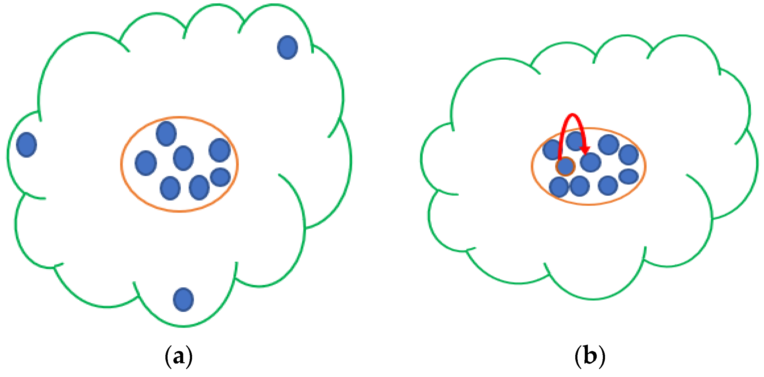
2.2.4. Problem of Early Convergence and Solution

If a model train/retrains for each entry or new arrival of data, the optimal solution vectors of a model may trap into one another after a certain cycle. The trapping reduces the effective solution population size, which can be understood from Figure 4. Figure 4a shows the initial condition or any random state of the solutions within the preferred solution boundary (green line). The orange circle can be considered as the global solution boundary as more solutions tend to reach that ball. Once all the solutions have reached the ball after a certain iteration, to minimize the distance between the best solution, there will be a possibility that one or more solutions trap into another solution, and that will effectively reduce the number of solutions (Figure 4b).

For example, if a system has a solution with a population size of 10, trapping into one of the solutions will reduce the effective population size to 9. Initially, trapping may suggest that the population vector has reached the global solution, but this may not always be true because metaheuristic algorithm performance is affected by the choice of hyperparameters. The selection of hyperparameters controls the speed of the population to move from one position to another. It may be possible that for the considered choice of hyperparameters, the solution vector may have missed any optimal location within the search space. Therefore, a modification in the application of metaheuristic has been proposed in this work; that is, whenever local trapping of one or more solutions occurs, a random solution against those solutions will be created within the search space, which in turn also create more opportunity to explore the search space. The modified portion of the algorithm is given in the Algorithm 1.

Algorithm 1 Duplicate Solution Removal Algorithm.

1: $\mathit{f}\mathit{o}\mathit{r} g=1:generation$ 2: $\mathit{f}\mathit{o}\mathit{r} p=1:population$ 3: $\mathit{i}\mathit{f} J\left(p,g\right)==J\left(q,g\right), Where p\ne q$ 4: $J\left(p,g\right)=x_{min}+rand\left(xmax-xmin\right)$ 5: $\mathit{e}\mathit{n}\mathit{d} \mathit{i}\mathit{f}$ 6: $\mathit{e}\mathit{n}\mathit{d} \mathit{f}\mathit{o}\mathit{r}$ 7: $\mathit{e}\mathit{n}\mathit{d} \mathit{f}\mathit{o}\mathit{r}$

2.3. Spearman’s Rank-Order Correlation Analysis

Spearman’s rank-order correlation analysis between variables a and b can be mathematically expressed as:

$$\rho \left(a,b\right)=1-\frac{6{\displaystyle \sum }{d}^2}{l\left(l^2-1\right)}$$

(10)

The variables a and b can be placed in two different columns of a table according to their sequence. The element of each variable a and b in the corresponding columns can be again ranked in ascending order, meaning that the highest and lowest value of a variable or column will be of the lowest and highest rank, respectively. The distance ($d$) of the variables a and b for any data $j$ can be simply calculated by $d_j$= rank($a_j$) − rank($b_j$). The numerical calculation procedure can also be obtained from Reference [50]. Spearman’s correlation coefficient value varies between –1 (perfect negative correlation) to +1 (perfect positive correlation). The operator can set a threshold of CC value to choose a dominant variable. If the absolute CC value exceeds the threshold, then the corresponding variable can be chosen, or else, it can be discarded from the optimization process. Mathematically,

$$\mathrm{input} \mathrm{variable}=\left\{a|\left|\rho \left(a,b\right)\right|\rangle th,\rho \left(a,b\right)ϵR\right\}$$

(11)

In this work, upon the arrival of each new data, the CC value will be updated. The procedure of dynamic analysis of the CC to determine the dominant input variables can be understood from Figure 5.

Figure 5 shows the change in CC between two variables with the change in data size. Analyzing the four quadrants of Figure 5a, it can be understood that, with the increase in data size (top left to bottom right), the CC also changes (from $0.82 \mathrm{to} 0.27)$. The change in CC values as per the change in data size or increase in number of days can be graphically plotted as shown in Figure 5b, where a threshold parameter has been shown using a red straight line. With respect to the threshold parameter, with time, as the dataset’s size grows, a variable may fluctuate around the state of dominance and non-dominance. By considering the state of dominance and non-dominance, the structure of the ANN can be adapted.

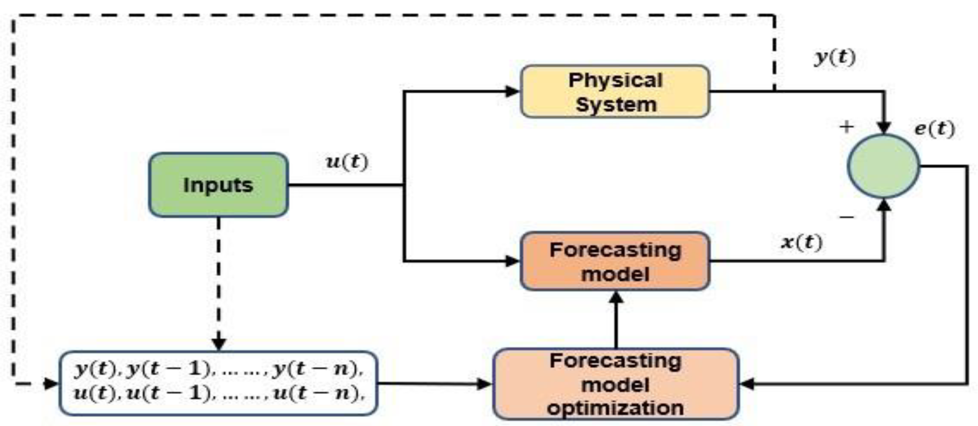
3. Proposed Algorithm for Dynamic Learning

In this section, the proposed algorithm is discussed, which is developed using the theories discussed in the previous section. The proposed algorithm is shown using the flowchart in Figure 6. The flowchart consists of 14 blocks, and in this section, the functions of each block are discussed briefly.

3.1. Block 1 (System Initialization)

In this block, the designer must decide the maximum possible number of input and output variables, the ANN network configuration (number of hidden layers, number of neurons in each layer, weights, biases, activation function, etc.), metaheuristic optimization hyperparameters, and total number of input combinations.

The total number of input combinations (Mode) can be mathematically expressed as:

$$Total number of Modes={\displaystyle \sum }_{\mathrm{y}=1}^n{n}_{C_y}=n_{C_1}+n_{C_2}+\dots \dots \dots +n_{C_n}$$

(12)

where $n$ is the number of input variables—the number of input variables in any ‘Mode’ may vary from one to $n$. A tabular description of the Mode is presented in

Table 4. Input combinations under different Modes for an arbitrary system.

Mode No	Inputs
	Variable 1	Variable 2	Variable 3	…..	Variable N
1	✔	✖	✖	✖	✖
2	✖	✔	✖	✖	✖
M	✔	✔	✔	✔	✔

.

Table 4 can be interpreted as such that if Mode 1 is chosen, input 1 is solely responsible for the system’s output change. Similarly, if Mode M is chosen, all the inputs are responsible for changes in the system output variable.

3.2. Blocks 2–6 (Data Collection and Sequential Entry, Feature Scaling and Correlation Analysis, Mode Consecutiveness Check)

In block 2, data from the electric grid (numerical weather data and synchronized plant power generation data) are taken and sequentially entered for dynamic learning purposes. Block 3 performs feature scaling to normalize the variables that are measured on different scales. Among many normalization methods, such as standard score, standardized moment, Min–Max feature scaling, etc. [51], Min–Max feature scaling has been selected. Mathematically, it can be expressed as:

$$Z^{\prime }=Y_{min}+\frac{\left(\mathrm{y}-X_{min}\right)\left(Y_{max}-Y_{min}\right)}{\left(X_{max}-X_{min}\right)}$$

(13)

The maximum–minimum value of input ($X_{max}, X_{min}$) and output ($Y_{max}, Y_{min}$) parameters needs to be updated at each sample entry as system knowledge is not a priori. In block 4, to choose a Mode from all possible Modes, CC analysis among the variables must be conducted. The consecutiveness of a Mode is checked in block 5. By consecutiveness analysis, if a Mode remains stable/unchanged for a predefined number of sample entries (z), the relation between an input and output variable can be considered to reach the steady-state condition. At this condition, the operator can stop the learning procedure (block 6) and conduct a comparative analysis of the model’s performance. In the flow chart, blocks 5, 6, 13, and 14 are represented with the dotted box. This means these blocks are optional, as one can continue to train the model for an infinitely long sequence of data entry.

3.3. Blocks 7–9 (Mode Occurrence Check, Solution Search Space Generation, and Evaluation of Model Performance)

If a Mode occurs for the first time, the algorithm will move to block 8 and generate a random solution according to the random distribution equation [52]. To generate a randomly distributed population programmatically, the following equation can be used:

$$\overrightarrow{x}=x_{min}+ran{d}_{no. of solutionsX1}\left(x_{max}-x_{min}\right)$$

(14)

where, $\overrightarrow{x}$ the initial uniform randomly generated solution vector, $ran{d}_{no. of solutionsX1}$ is a uniform distribution column vector, and $x_{max}$ and $x_{min}$ are boundary values of the initial search space.

If the Mode occurred for m^th times (m|1 < m < z), the algorithm will move to block 9. Then, the model performance under the current data entry will be evaluated using the optimal solution from the Mode’s previous occurrence, which increases the probability of faster convergence. Mathematically,

$${\stackrel{\rightharpoonup }{X_0}}_{\mathrm{m}}^M={\stackrel{\rightharpoonup }{X_{0pt}}}_{\mathrm{m}-1}^M$$

(15)

${\stackrel{\rightharpoonup }{X_0}}_j^M$ and ${\stackrel{\rightharpoonup }{X_{0pt}}}_{j-1}^M$ are the initial solution and optimized solution vector of Mode M, respectively.

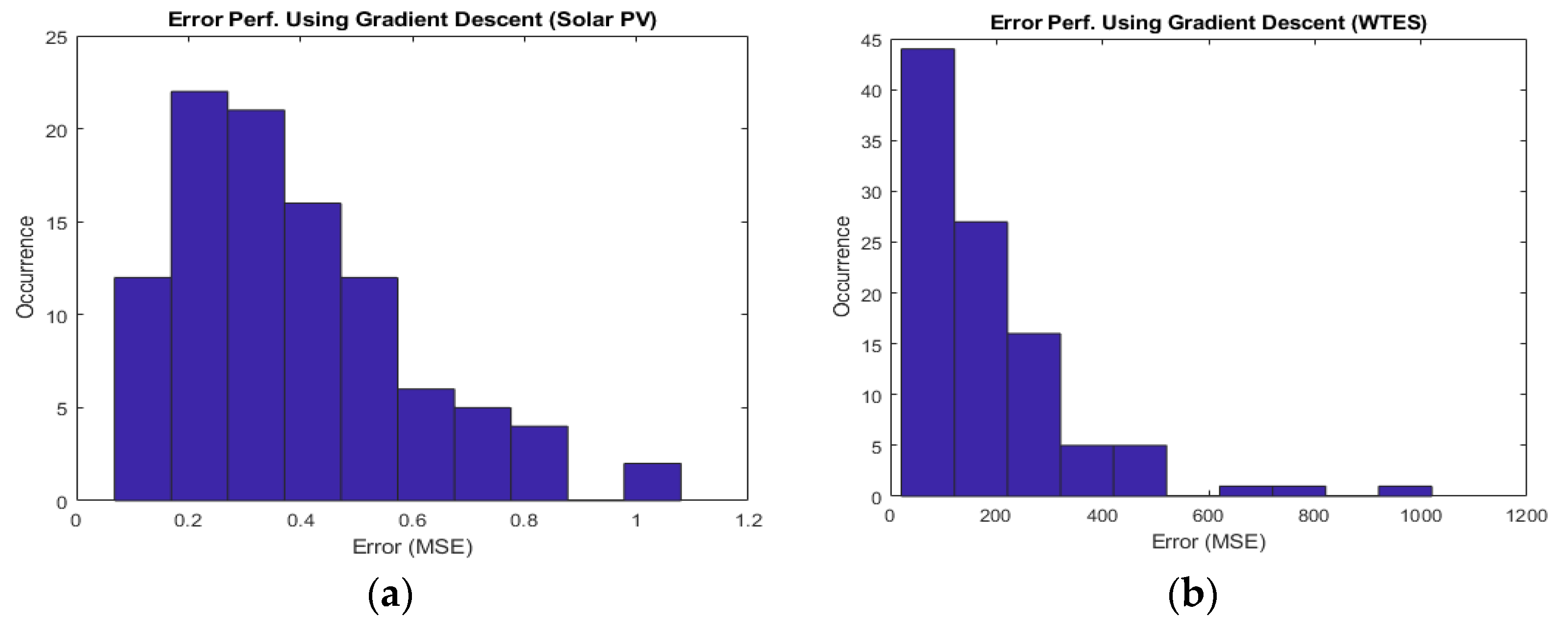
3.4. Blocks 10–14 (Error Analysis, MAANN Optimization, Storing the Best Solution, Statistical Analysis, and Choosing the Best Algorithm)

Block 10 evaluates the error using MSE, and if MSE is found to be more than a predefined value ($eph$), the model will go into the optimization process in block 11 (tuning of MAANN weights and biases). If the error is less than the $eph$, the optimization will be skipped to avoid model overfitting and maintain the model generalization. Mode-specific optimal solution prevents the system from generating random solutions periodically; therefore, learning will be faster. The Mode-specific optimal results will be stored in Mode-specific ANN weights and bias matrix and vectors in block 12, which will be ready for reuse when new data arrives.

After stopping the learning procedure, the performance of different models (optimization methods) is evaluated in block 13, and the best model will be selected (block 14). For the model performance evaluation, along with the MSE, the following indexes are used:

$$\begin{gathered} Bayesian Information Criterion, \mathrm{BIC}=\ln \left(l\right)k^{\prime }-2\ln \left(\widehat{L}\right) \\ = l log\left(\frac{\mathrm{SSE}}{l}\right)+\mathrm{P}log l \end{gathered}$$

(16)

$$Standard Deviation, \sigma =\sqrt{\frac{{\displaystyle \sum }{\left(x_j-\mu \right)}^2}{l}}$$

(17)

$$R-value, R^2=1-\frac{{{\displaystyle \sum }}_{j=1}^l{\left({\widehat{Y}}_j-Y_j\right)}^2}{{{\displaystyle \sum }}_{j=1}^l{\left({\widehat{Y}}_j-\frac{1}{l}{{\displaystyle \sum }}_{j=1}^{l}Y\right)}^2}$$

(18)

$$\mathrm{Mean} \mathrm{Absolute} \mathrm{Error}, \mathrm{MAE}=\frac{1}{l}{\displaystyle {\sum }_{j=1}^l}\left|{\widehat{Y}}_j-Y_j\right|$$

(19)

$$\mathrm{The} \mathrm{standard} \mathrm{deviation} \mathrm{of} \mathrm{the} \mathrm{error}, \mathrm{SDE}=\sqrt{\frac{1}{l}{{\displaystyle \sum }}_{j=1}^l{\left(Erro{r}_j-Mean Error\right)}^2}$$

(20)

BIC [53] measures the distance between the actual data and the model. The lesser the distance, the better the model is. The second equation in (16) is the equivalent of the original equation for neural network-based application. For the population-based algorithms, complete or near convergence to a solution of all the particles can be defined as the optimal solution. At the optimal condition, the solution boundary will be significantly small, which also provides a smaller standard deviation. Hence, standard deviation is measured as an index to optimal solution convergence. R-value is used to demonstrate the fitting of the model. Finally, the MAE and SDE are used to measure the error of the model. The smaller the MAE and SDE, the better the model is.

4. Experimental Validations

In this work, the proposed algorithm’s effectiveness has been demonstrated by applying two different renewable energy sources of two different places. The wind dataset has been collected from the NREL website [54] for 2012, near New Kirk. The original dataset consists of power, wind direction, wind speed, air temperature, surface air pressure, and air density. The later five (wind direction, wind speed, air temperature, surface air pressure, and air density) were considered as the input variables, and power was considered as the variable to be forecasted.

Similarly, the dataset was collected from the Republic of Korea’s public data website [55] for the Yeongam F1 Stadium for the Solar PV system. The data is obtained for three years and ten months from January 2015 to October 2018. Inclined irradiance, surface temperature, and surrounding temperature from the dataset were considered as the input variables, while plant output power was considered as the predicting variable. The details of the dataset are given in

Table 5. Dataset specifications.

WTES (New Kirk-Site ID: 19287)		PV (Yeongam F1 Stadium 1 Electrical Room)
Parameters	Numerical values	Parameters	Numerical Values
Plant Maximum Output	16 MW	Plant Maximum Output	2610 kW
Maximum Wind Speed	23.0352	Plant Capacity	3026 kW
Maximum Wind Direction	359.3794 degrees	Maximum Inclined Irradiance	999.96
Maximum Temperature	35.9660 degrees Celsius
Maximum air Pressure	8.5927 × 104 Pa	Maximum Surface Temperature	49.78
Maximum air density	1.0980 Kg/m3
Longitude	−104.258	Maximum Surrounding Temperature	125.60
Latitude	35.00168
Duration	(1 Year) 2012	Duration	3 years, 10 months (2015 to 2018)
Time Interval	5 min	Time interval	1 h
No of datapoints	105,116	Data points	17,252

.

4.1. Initialization of Experimental Setup

To initiate the experiments, the chosen ANN structure and metaheuristic algorithm hyperparameter settings are provided in

Table 6. ANN parameters’ default values of the experiment.

Parameters	Initial Solution Search Space	Number of Input Layer Weights (n, Number of Inputs)	Number of Input Layer Biases	Number of Output Layer Weights	Number of Output Layer Biases	Number of Hidden Layers
Values	(−5, 5)	$n$ × 10	10	10	1	1

and

Table 7. Parameter settings of different metaheuristic algorithms.

Algorithm	Parameter	Values	Population Size	Max Generation
APSO	$C_1,C_2,w$	1.5, 1.5, 0.9	20	10
Jaya	$Not Required$	-
FTMA	$p,r$	0.7, 0.7

. These experiments have been conducted in a PC with Intel^® Core (TM) i7-6700 CPU @3.40 GHz processor in MATLAB 2018a.

The structure (number of weights, biases, hidden layers) choice of the activation function (hyperbolic tangent) has been taken the same as the gradient descent-based algorithm, which was developed and applied through the MATLAB built-in toolbox. Keeping the same structure makes the systems comparable on the same ground.

According to Figure 6, the initial model’s error should be more than a tolerance value ($eph$) to start the optimization. Error tolerance is a designer parameter, meaning that the designer can choose a relatively small value, below which the optimization cycle will not be initiated.

To choose the error limit/tolerance ($eph$), the minimum error achieved by applying a gradient descent technique on the ANN for the given dataset has been chosen. To do that, ANN has been trained exactly 100 times for each dataset, and the minimum error from that simulation is set as an error threshold for the metaheuristic optimization-based method. In Figure 7, the histogram of the error from the gradient descent-based training of the dataset is shown. From the figure, the minimum of the error for solar PV and WTES was found as 0.0682 and 6.2096 respectively, which are used as the error limit/tolerance ($eph$) for the metaheuristic-based model training.

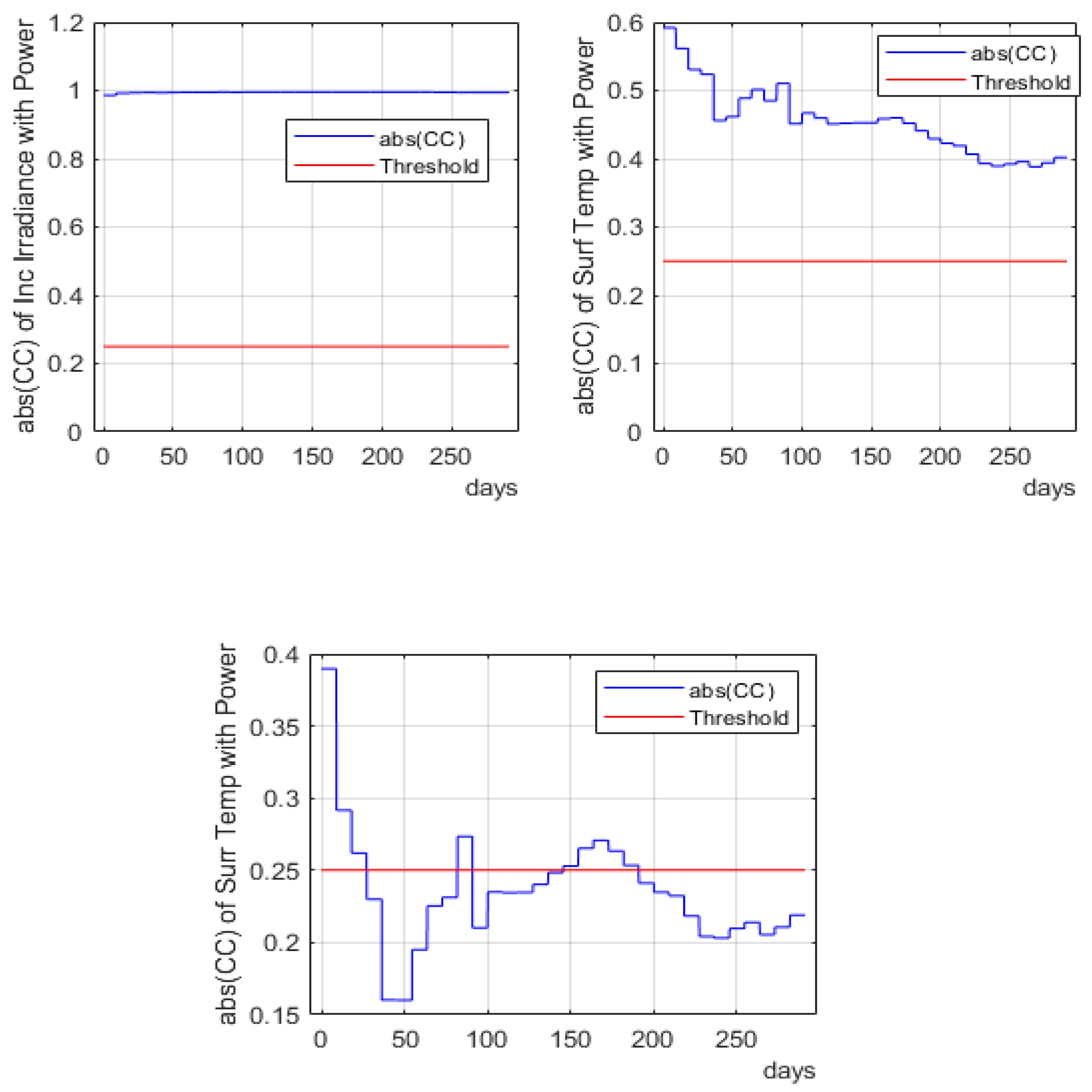
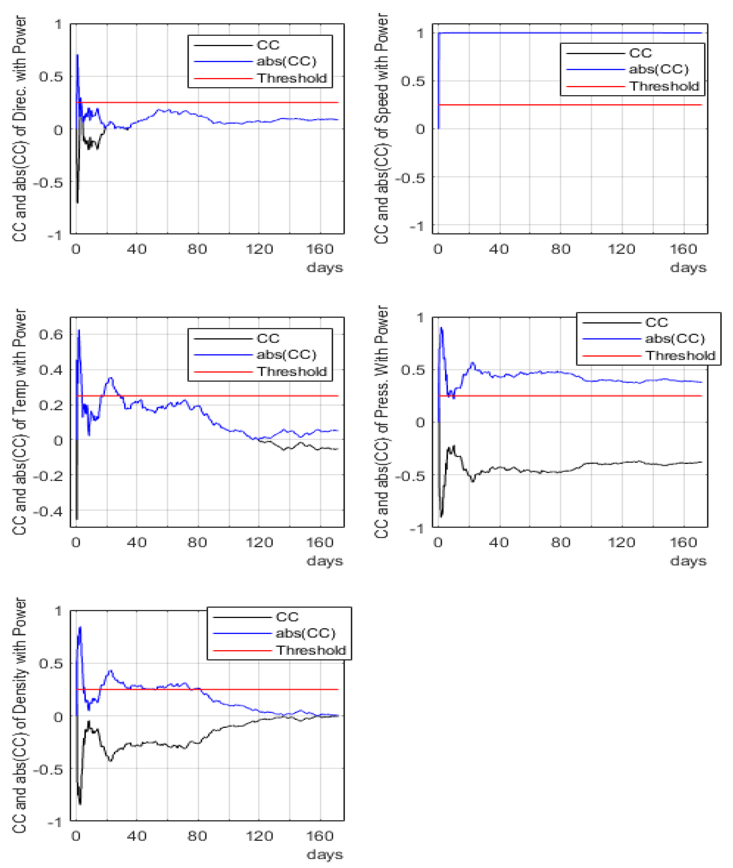
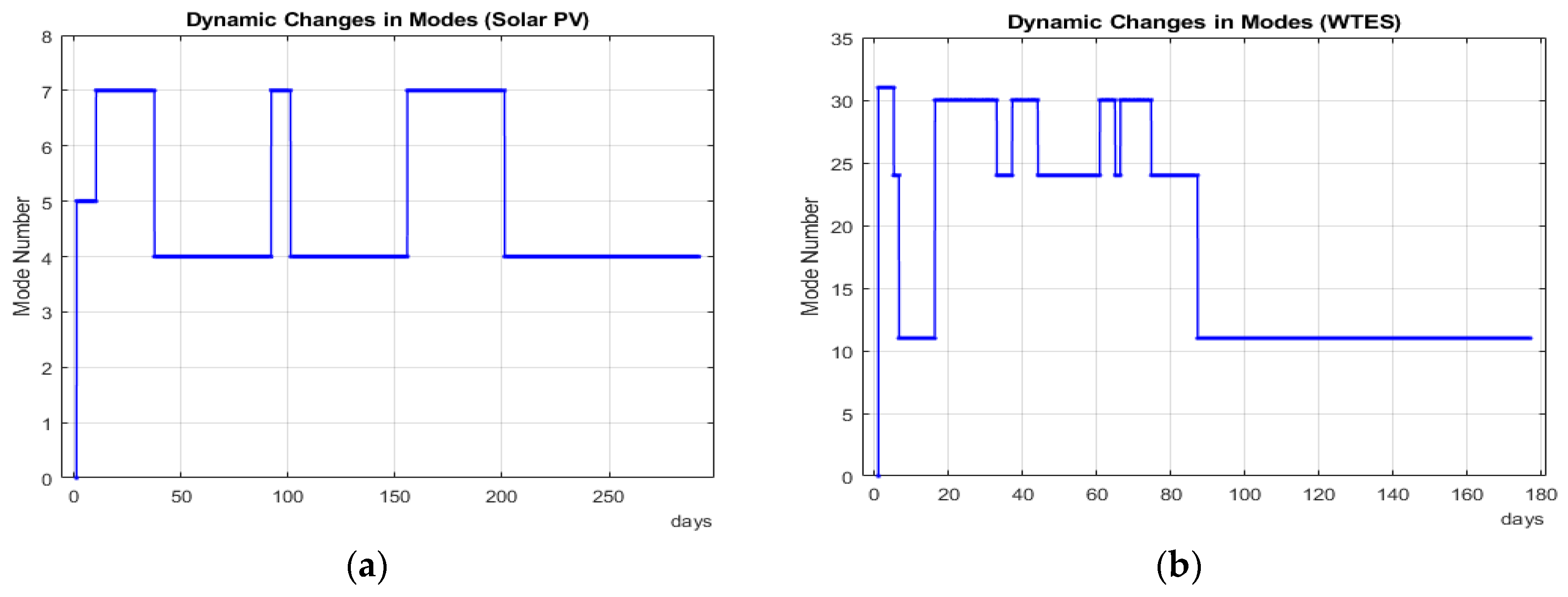
4.2. Dynamic Change in CC and Mode Analysis

The dynamic plotting of the actual and absolute value of the CC of power output to each input variable is presented in Figure 8 and Figure 9. The CC threshold is also presented with the figures to indicate the change in dynamics of CC over time. For solar PV system, actual and absolute CC are both positive; however, for WTES, some quantities are found in the negative and positive range also. Therefore, to maintain uniformity across the models, absolute value has been considered.

Generally, CC between $\pm$0.75 to $\pm$1 is considered as very strong, $\pm$0.50 to $\pm$0.75 as moderate, $\pm$0.25 to $\pm$0.50 as weak, and below that has no association [56]. Therefore, in this work, the absolute threshold for CC analysis has been set as 0.25. Hence, any variable with the CC below 0.25 is discarded as a dominant input variable. Figure 8 shows that the absolute CC of inclined irradiance and surface temperature always remains above the threshold line. In contrast, the absolute CC for the surrounding temperature varies around the threshold line and becomes a non-dominant variable at the end.

For WTES, wind speed and air pressure were mostly above the threshold value, and that makes them dominant variables at the end of model training, whereas the other variables oscillate around the threshold, making them temporarily choice variables, but their dominance vanishes as the data size grows. According to actual CC analysis, pressure has a negative CC value, which means that power generation decreases with the increase in pressure.

The data source countries’ (South Korea/USA) weather can be classified according to 4 seasons (three months/season). Thus, the consecutiveness of a Mode for three months is considered as the stable dataset size and training stopping criteria. The training started from January’s data, which is the second/third month of winter in the considered countries; thus, considering three months for stopping criteria overlaps two different seasons. The stopping criteria validate the stability of the dataset according to the use of CC. Analyzing the dynamic CC along with the threshold line, dynamic changes in the Modes can be obtained from Figure 10.

For the solar PV system, occurred Modes are 5 (inclined irradiance, surrounding temperature), 7 (inclined irradiance, surface temperature, surrounding temperature), and 4 (inclined irradiance, surface temperature). Among them, the stable Mode was 4. For WTES, occurred modes are 31 (direction, speed, temperature, pressure, density), 24 (speed, pressure, density), and 11 (speed, pressure), 30 (speed, temperature, pressure, density). Among them, 11 is the stable one. The complete Mode table is given in the Appendix A, where

Table A1. Mode selection table for Solar PV system.

Mode Number	Inputs
	Inclined Irradiance	Surface Temperature	Surrounding Temperature
1	✔	✖	✖
2	✖	✔	✖
3	✖	✖	✔
4	✔	✔	✖
5	✔	✖	✔
6	✖	✔	✔
7	✔	✔	✔

is for Solar PV, and

Table A2. Mode selection table for WTES.

Mode Number	Inputs
	Direction	Speed	Temperature	Pressure	Density
1	✔	✖	✖	✖	✖
2	✖	✔	✖	✖	✖
3	✖	✖	✔	✖	✖
4	✖	✖	✖	✔	✖
5	✖	✖	✖	✖	✔
6	✔	✔	✖	✖	✖
7	✔	✖	✔	✖	✖
8	✔	✖	✖	✔	✖
9	✔	✖	✖	✖	✔
10	✖	✔	✔	✖	✖
11	✖	✔	✖	✔	✖
12	✖	✔	✖	✖	✔
13	✖	✖	✔	✔	✖
14	✖	✖	✔	✖	✔
15	✖	✖	✖	✔	✔
16	✔	✔	✔	✖	✖
17	✔	✔	✖	✔	✖
18	✔	✔	✖	✖	✔
19	✔	✖	✔	✔	✖
20	✔	✖	✔	✖	✔
21	✔	✖	✖	✔	✔
22	✖	✔	✔	✔	✖
23	✖	✔	✔	✖	✔
24	✖	✔	✖	✔	✔
25	✖	✖	✔	✔	✔
26	✔	✔	✔	✔	✖
27	✔	✔	✔	✖	✔
28	✔	✔	✖	✔	✔
29	✔	✖	✔	✔	✔
30	✖	✔	✔	✔	✔
31	✔	✔	✔	✔	✔

is for WTES. Greyed boxes represent the Modes that appeared during the training process.

4.3. Data Entry (Episode)-Wise Optimization Algorithms Performance Comparison

Each entry or arrival of new data and the corresponding cycle of model optimization has been defined as an episode. In Figure 11, episode-wise error reduction performance of the three algorithms has been shown simultaneously.

Figure 11 shows that the models optimized with different algorithms are reaching the acceptable error performance towards the end of the training period. Due to the three levels of optimization process (randomization, exploration, exploitation), FTMA performs considerably better than the other two metaheuristic algorithms for both cases. Whereas, the Jaya algorithm with no hyperparameter being relatively simple could not reach better solutions than the other two algorithms. It can be mentioned that, at times, due to the appearance/reappearance of a new/previous mode, the error was increasing too. Because, at the first appearance of a new Mode, optimization starts with a random solution vector, which may not be optimal. Also, the reappearance of a Mode after a long time (meaning that not trained with the recent data entries) may produce a larger error. However, as the training dataset size increases, with multiple training loops, the error reduces gradually.

The error reduction performance of each optimization algorithm can be more clearly understood from the episode-wise winner analysis graph of Figure 12. Upon the arrival of each/set of new data, the optimization method with the best error reduction performance can be selected as the episode winner after performing the training. For episode-wise winner analysis, each algorithm was assigned with a weighted value. APSO, Jaya, and FTMA were assigned with 1, 2, and 3, respectively. For both cases (Solar PV and WTES), FTMA has won the maximum number of episodes. The numbers are shown in

Table 8. Results for Solar PV.

Algorithms	MSE (MW2)		RMSE (MW)		BIC(−1 × 104)		MAE (MW)
	Training	Testing	Training	Testing	Training	Testing	Training
APSO	0.0684	0.0714	0.2615	0.2672	0.8007	0.0819	0.1941
JAYA	1.1204	1.5149	1.0584	1.2308	−0.0938	−0.0635	0.8639
FTMA	0.0196	0.0207	0.14	0.1438	1.2008	0.1399	0.1034
Gradient Descent	0.0682	0.0256	0.2611	0.16	−0.1704	0.1273	0.8405
ARIMAX	0.0230	0.0660	0.1516	0.2569	0.8357	0.1347	0.9362
	Standard Deviation	R-Value		Episode Winner	SDE (MW)		MAE (MW)
		Training	Testing		Training	Testing	Testing
APSO	13.0717	0.9519	0.9565	45	14.7976	5.7798	0.1950
JAYA	3.3917	0.2128	0.0764	0	59.8978	26.8282	1.0277
FTMA	0.0075	0.9863	0.9874	245	7.9161	3.1352	0.1005
Gradient Descent	-	0.9669	0.9871	-	59.4784	3.5814	0.1363
ARIMAX	-	0.9838	0.9659	-	66.6497	27.5989	1.0272

and

Table 9. Results for WTES.

Algorithms	MSE (MW2)		RMSE (MW)		BIC(1 × 104)		MAE (MW)
	Training	Testing	Training	Testing	Training	Testing	Training
APSO	1.4439	2.3080	1.2	1.5192	1.9352	0.6071	0.9574
JAYA	22.5438	22.1656	4.7480	4.7080	1.5825	2.3591	3.9185
FTMA	1.21	0.4944	1.1	0.7031	1.056	−0.4996	0.7283
Gradient Descent	6.2096	8.1727	2.4919	2.858	22.694	1.3718	6.7104
ARIMAX	9.3338	7.7290	3.055	2.780	−31.955	−4.5964	7.4354
	Standard Deviation	R-Value		Episode Winner	SDE (MW)		MAE (MW)
		Training	Testing		Training	Testing	Testing
APSO	1.4439 × 103	0.9835	0.9616	66	271.1004	131.8828	1.2750
JAYA	12.9087	0.7424	0.6317	0	1.0712 × 103	409.1466	4.1227
FTMA	65.0949	0.9861	0.9918	109	248.5482	60.6081	0.4939
Gradient Descent	-	0.9221	0.9122	-	708.6053	210.9264	1.9018
ARIMAX	-	0.8934	0.9170	-	799.3252	667.8077	6.2505

.

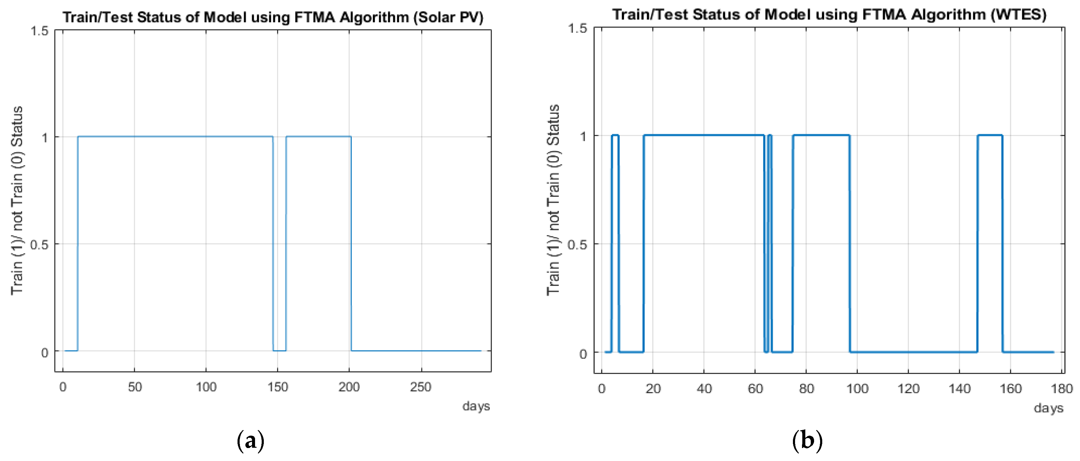
4.4. Train/Test Status of the Algorithm

The train/test status indication figure proves the effectiveness of the proposed algorithm and FTMA. As the best error performance of the gradient descent algorithm has been taken as the error limit, therefore, if the error reduction by metaheuristic algorithms is found better, the MAANN will avoid optimization. This indicates that the trained models are showing better performance than the conventional approach (gradient descent). Figure 11 and Figure 12 show that the FTMA outperforms the other two algorithms. Hence, the train/test status of the FTMA algorithm is only shown in Figure 13. Train/test status analysis is essential for understanding how the model can participate in the electricity market and earn more profits. The data specification table shows that the Solar PV data is collected for 3 years and 10 months, and WTES data were collected for one year. However, using the data stability condition, Solar PV and WTES training were stopped around the 290th and 177th days respectively, which is far less than the actual dataset size.

Also, from Figure 13, it can be found that, due to efficient training using the FTMA algorithm, the training cycle can be avoided in many instances (showing as 0 state in the figure). This means as the error is reduced, the model can successfully participate in the electricity market and earn profits. However, the participation should be stopped once the model performance exceeds the error threshold and reoptimizes it. Following that, if the next entries’ error goes below the threshold quantity, the model will again participate in the market. This phenomenon can be explained by Figure 13b. For example, the model error of the WTES system around the 96–146th day is less than the threshold quantity; therefore, the model can participate in the market and earn a profit, but after the 146th day, the error again exceeds the threshold. Hence, the model should reoptimize again and stop participating in the electricity market. Again, around the 157th day, the error has been reduced to an acceptable limit. Consequently, the energy producer can participate in the market again.

4.5. Time Analysis of the FTMA

As metaheuristic algorithms are population-based methods, it may take a long time to reach an acceptable solution. Thus, the training time using the metaheuristic algorithms is always a concern for the designers. FTMA has better error reduction performance, and it is the winner of the maximum number of episodes; therefore, the time required for the algorithm with FTMA optimization is shown in Figure 14. It is understandable that, with the increase in data size, the training time will be increased. Thus, the help of the MATLAB parallel computation toolbox has been taken to reduce the optimization time. The use of the MATLAB parallel computing toolbox keeps the training time maximum of 91 s for the Solar PV and 168.3123 s for the WTES, whereas the mean training time was 26.13 and 48.84 s, respectively. The training time peaks occur due to the presence and removal of duplicate solutions to maintain the effective number of solutions uniform. It is found that the model average training time is much smaller than the data sample interval (1 h for Solar PV and 5 min for WTES). Hence, the algorithm can be easily applied to the system.

4.6. Solution Convergence Analysis of Different Optimization Algorithms

The convergence of the solution vectors’ population can be seen from the box-plot analysis of Figure 15. Compared to the APSO and Jaya algorithms, the population from the solution vector of FTMA has reached the optimal state for the Solar PV system. As the population of FTMA is located very near to each other, therefore, standard deviation for FTMA (0.0075) is much smaller than the APSO (13.0717) and Jaya algorithms (3.3917). For WTES, Jaya and FTMA are found to have a better convergence state compared to APSO. Although FTMA has achieved the minimum error, to avoid duplicate solution, one of the solutions (red cross) appeared a little away from the solution cluster. Thus, the standard deviation of FTMA (65.0949) is more than the Jaya algorithm (12.9087).

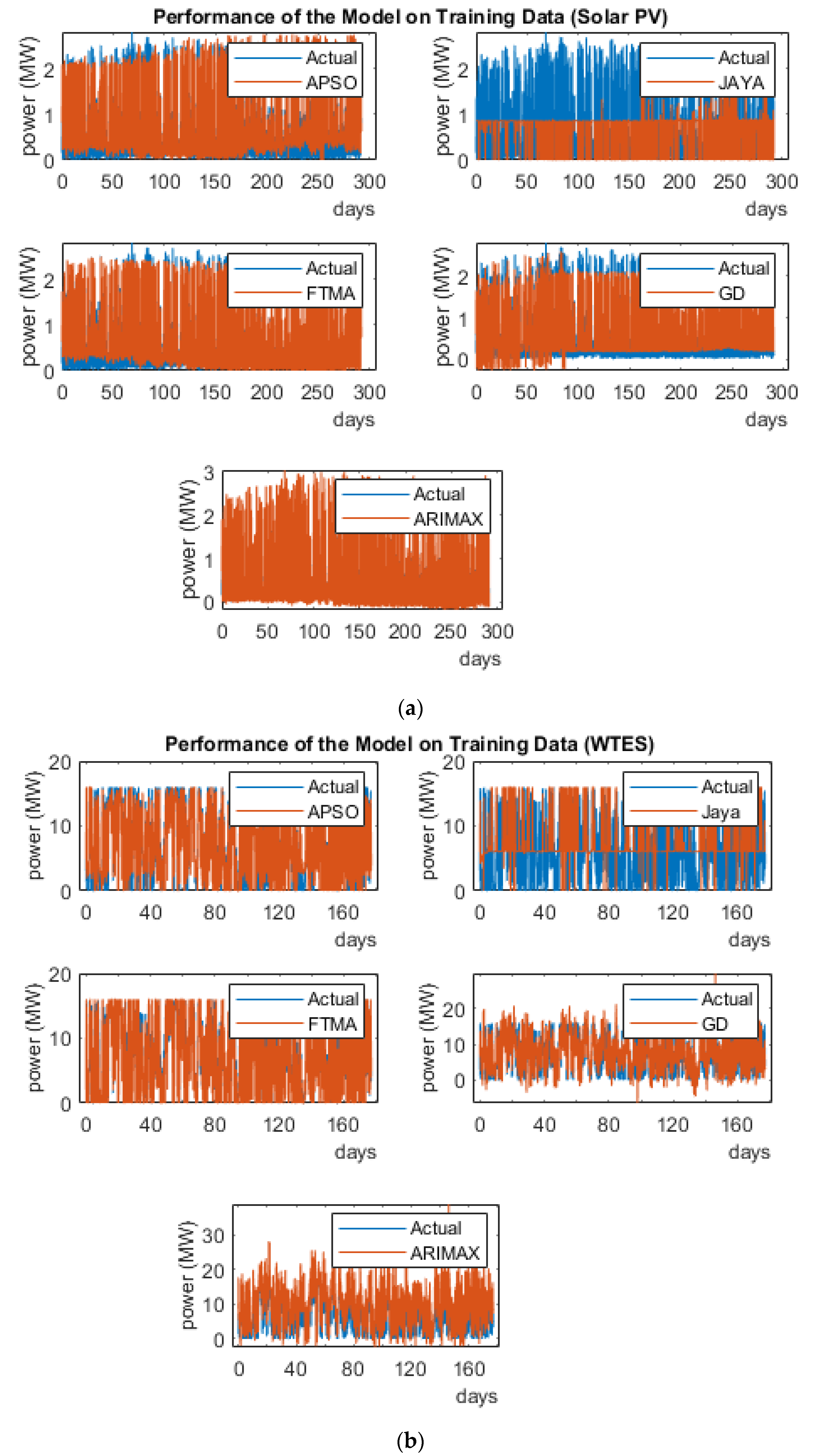
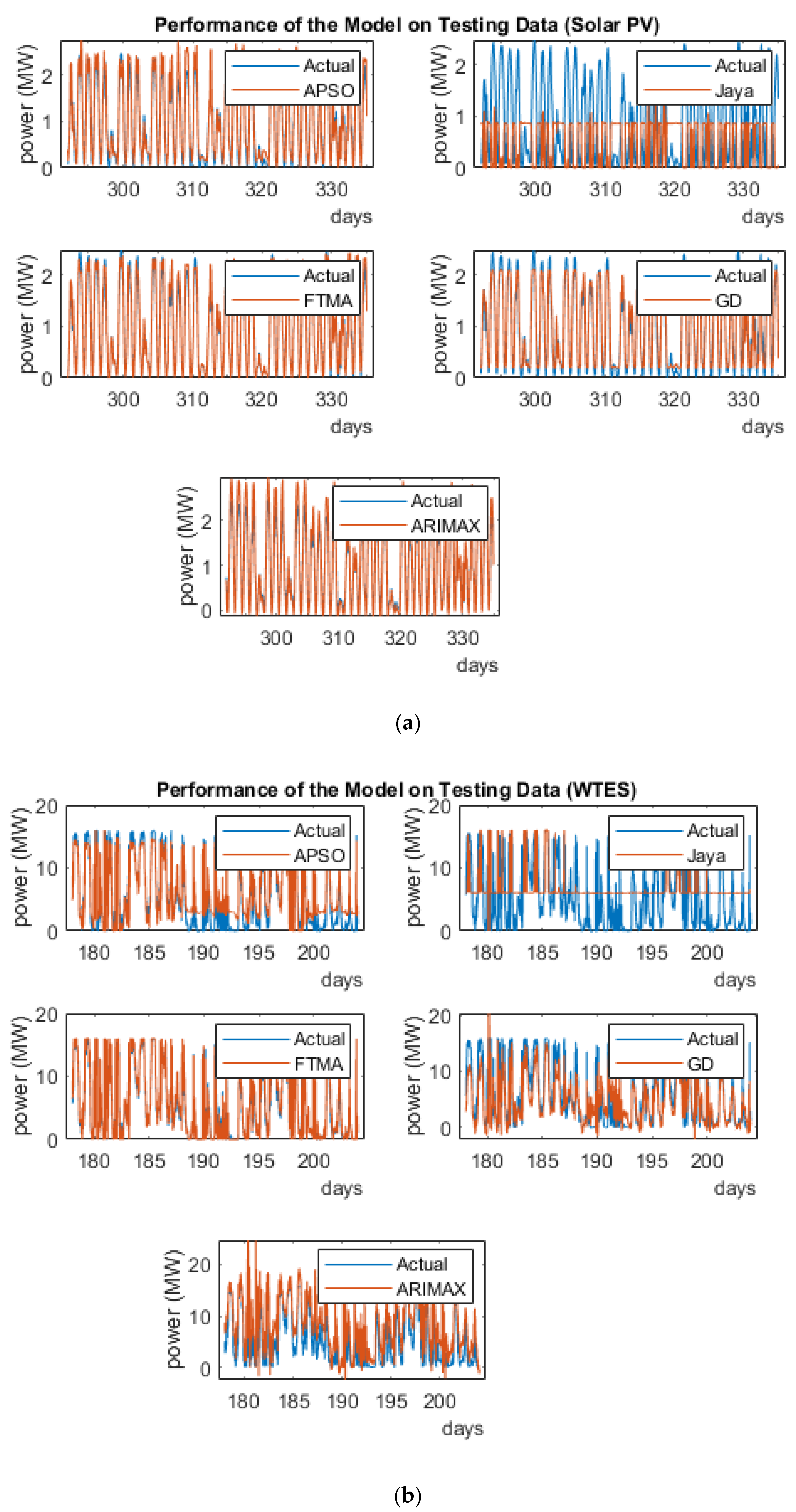
4.7. Comparison of Training and Test Dataset

In this subsection, the training and testing set results have been shown in Figure 16 and Figure 17, respectively. Blue lines are used as the original data, and the brown lines are used as the output of different trained models. The errors between the actual outputs and the trained model outputs are calculated using MSE, RMSE, and MAE. Corresponding values for training and testing datasets are shown in Table 8 and Table 9. Also, using the original and trained model data, R-value is calculated using Equation (18) and presented in Table 8 and Table 9. For both cases, FTMA and APSO perform relatively better than Jaya and gradient descent-based algorithms. In addition to the gradient descent-based method, the algorithms were compared with ARIMAX, a non-neural network-based algorithm. ARIMAX was implemented with the econometric toolbox in MATLAB.

As in this work, a MATLAB-based toolbox is used for base case (gradient descent) training, and by default, the toolbox partitions 15% of the data as a testing dataset. Therefore, whenever the algorithm termination criteria are satisfied based on the data stability, the algorithms’ performances are validated by applying to the testing dataset, which is nothing but 15% of additional data points of the ending point of the training data. For example, Solar PV system training stopped at the 290th day; hence, the testing horizon is considered as 290 + 290 × 0.15 $\approx$ 334 days, and for WTES, 177 + 177 × 0.15 $\approx$ 204 days. Therefore, in Figure 16, the performance of the trained model on the training dataset (0–290th day for Solar PV and 0–177th day for WTES), and in Figure 17, the performance of the same model on the testing dataset (290–334th day for Solar PV and 177–204th day for WTES) has been shown. It should be mentioned that the testing data horizon is a designer parameter that can be varied, and the performance of the algorithm can be analyzed too. In practice, the training and testing cycle should occur according to the methodology discussed in Section 4.4.

4.8. Tabular Comparison

The performance and robustness of the algorithm and the optimization methods are verified using multiple performance indexes (MSE, RMSE, SDE, MAE, BIC, Standard Deviations, R-value, and the number of episode winners) and shown in Table 8 and Table 9. The grey boxes show the best performance achieved among the algorithms, where RMSE is nothing but the square root of MSE, because the unit of MSE is the square unit of the output quantity (MW²), where RMSE has the same as the output (MW), which makes it easily comprehensible. In terms of MSE, RMSE, MAE, SDE, and R-value, and the number of episode winners, FTMA has performed better than other algorithms for both cases (Solar PV and WTES). As mentioned in Section 3, the smaller the BIC is, the better the model is. However, looking carefully at the Table 8 shows that the Solar PV system’s BIC order is negative (−1 × 10⁴). As the sign convention is negative, the bigger the positive value inside the table, the better the model will be. Hence, FTMA was found to be better in terms of BIC for the solar PV system. However, for BIC of the WTES system, ARIMAX has performed better than other algorithms.

Also, the standard deviation as an index for the convergence of the optimization algorithms shows that FTMA has performed better in the case of Solar PV systems, whereas in the case of the WTES, the Jaya algorithm performed better. As the gradient descent-based algorithm and ARIMAX are not a population-based methodology, therefore, the standard deviation and episode-wise winner block is kept blank. By numerical calculation, it can also be found that error using FTMA is reduced, $\frac{0.0682-0.0196}{0.0682} \times 100=71.261\%$ $\frac{6.2096-1.21}{6.2096}\times 100=80.514\%$ of the gradient descent algorithm in the case of Solar PV and WTES, respectively.

Therefore, it can be said that the proposed algorithm with a suitable optimization algorithm can perform better than the conventional gradient descent or ARIMAX algorithm, which is FTMA in this case study. The major advantage is, as the proposed algorithm is a dynamic approach, the model can start participating in the electricity market from the beginning depending on the error performance. It is also found that training accuracy is increased, and learning time is decreased (train/test status) due to dynamic learning.

5. Conclusions and Future Work

In this work, a Mode Adaptive Artificial Neural Network has been proposed for the dynamic learning of renewable energy sources power generation prediction. The dynamic learning using Spearman’s rank-order correlation provides a logical solution to choose the correct dominant inputs over time, which is found as a suitable tool for data stability analysis, too. As the model dynamically learns the system over a long period, therefore, different forecasting horizons (short, medium, long)-based modeling strategies can be avoided. FTMA was found better among the optimization algorithms due to its three-level algorithmic architecture, and provided better accuracy in every cycle.

The use of multiple performance indexes shows the robustness of the proposed algorithm using FTMA over other algorithms. Also, using FTMA, error has been reduced by 71.261% and 80.514% compared to the fixed-sized data-based trained model using the gradient descent algorithm. This also proves the benefit of dynamic/online learning over a conventional fixed-sized data-based learning approach.

One of the major concerns of the proposed algorithm is the choice of optimization algorithm and the respective hyperparameters. An increase in population and generation number may yield better results but at the cost of time. In the future, unlike this work, the verification of the proposed model should be conducted for multi-plant forecasting model development. In this work, testing was performed for instantaneous values of the input variables, which in the future can be easily extended for delayed input variables by performing auto- and cross-correlation.

In the future, this algorithm can be applied with the actual system installed in any geographical location. The model will be trained and participate in the electricity market without prior knowledge or training. In this work, the considered input variables were all continuous; in the future, systems with discrete variables can be considered by incorporating discrete to continuous CC analysis tools. Also, in contrast to the current approach, in the future, a unified feature reduction and forecasting approach can be taken, which will reduce the model complexity. The proposed algorithm can also be applied to any general case of real-time model learning, such as the share market. The algorithm can also be applied for load and EV modeling, as they are dependent on many external factors (variables). In brief, it can be concluded that the proposed algorithm can break the barrier of fixed-sized data training and help the operator to gain more profits by early participation in the market. Also, as in this problem, ANN’s simple architecture has been adopted, therefore, it can be applied in any developing/under-developing countries where high processing computers are expensive for DL technologies.

References

1. Saberian, A.; Hizam, H.; Radzi, M.A.M.; Ab Kadir, M.Z.A.; Mirzaei, M. Modelling and Prediction of Photovoltaic Power Output Using Artificial Neural Networks. Int. J. Photoenergy 2014, 2014. [Google Scholar] [CrossRef] [Green Version]
2. Abuella, M.; Chowdhury, B. Solar power forecasting using artificial neural networks. In Proceedings of the 2015 North American Power Symposium (NAPS), Charlotte, NC, USA, 4–6 October 2015. [Google Scholar] [CrossRef]
3. Qasrawi, I.; Awad, M. Prediction of the Power Output of Solar Cells Using Neural Networks: Solar Cells Energy Sector in Palestine. Int. J. Comput. Sci. Secur. 2015, 9, 280. [Google Scholar]
4. Alomari, H.M.; Younis, O.; Hayajneh, M.A.S. A Predictive Model for Solar Photovoltaic Power using the Levenberg-Marquardt and Bayesian Regularization Algorithms and Real-Time Weather Data. Int. J. Adv. Comput. Sci. Appl. 2018, 9. [Google Scholar] [CrossRef] [Green Version]
5. Theocharides, S.; Makrides, G.; Georghiou, E.G.; Kyprianou, A. Machine learning algorithms for photovoltaic system power output prediction. In Proceedings of the 2018 IEEE International Energy Conference (ENERGYCON), Limassol, Cyprus, 3–7 June 2018. [Google Scholar] [CrossRef]
6. Al-Dahidi, S.; Ayadi, O.; Adeeb, J.; Louzazni, M. Assessment of Artificial Neural Networks Learning Algorithms and Training Datasets for Solar Photovoltaic Power Production Prediction. Front. Energy Res. 2019, 7. [Google Scholar] [CrossRef] [Green Version]
7. Khandakar, A.; Chowdhury, E.H.M.; Khoda Kazi, M.; Benhmed, K.; Touati, F.; Al-Hitmi, M.; Gonzales, S.P.A., Jr. Machine Learning Based Photovoltaics (PV) Power Prediction Using Different Environmental Parameters of Qatar. Energies 2019, 12, 2782. [Google Scholar] [CrossRef] [Green Version]
8. Su, D.; Batzelis, E.; Pal, B. Machine Learning Algorithms in Forecasting of Photovoltaic Power Generation. In Proceedings of the 2019 International Conference on Smart Energy Systems and Technologies (SEST), Porto, Portugal, 9–11 September 2019. [Google Scholar] [CrossRef]
9. Velasco, N.J.; Ostia, F.C. Development of a Neural Network Based PV Power Output Prediction Application Using Reduced Features and Tansig Activation Function. In Proceedings of the 2020 6th International Conference on Control, Automation and Robotics (ICCAR), Singapore, 20–23 April 2020. [Google Scholar] [CrossRef]
10. Gensler, A.; Henze, J.; Sick, B.; Raabe, N. Deep Learning for solar power forecasting—An approach using AutoEncoder and LSTM Neural Networks. In Proceedings of the 2016 IEEE International Conference on Systems, Man, and Cybernetics (SMC), Budapest, Hungary, 9–12 October 2016. [Google Scholar] [CrossRef]
11. Poudel, P.; Jang, B. Solar Power Prediction Using Deep Learning Technique. Adv. Future Gener. Commun. Netw. 2017, 146, 148–151. [Google Scholar]
12. Hua, C.; Zhu, E.; Kuang, L.; Pi, D. Short-term power prediction of photovoltaic power station based on long short-term memory-back-propagation. Int. J. Distrib. Sens. Netw. 2019. [Google Scholar] [CrossRef]
13. Dawan, P.; Sriprapha, K.; Kittisontirak, S.; Boonraksa, T.; Junhuathon, N.; Titiroongruang, W.; Niemcharoen, S. Comparison of Power Output Forecasting on the Photovoltaic System Using Adaptive Neuro-Fuzzy Inference Systems and Particle Swarm Optimization-Artificial Neural Network Model. Energies 2020, 13, 351. [Google Scholar] [CrossRef] [Green Version]
14. Zhu, H.; Lian, W.; Lu, L.; Dai, S.; Hu, Y. An Improved Forecasting Method for Photovoltaic Power Based on Adaptive BP Neural Network with a Scrolling Time Window. Energies 2017, 10, 1542. [Google Scholar] [CrossRef] [Green Version]
15. Le Cadre, H.; Aravena, I.; Papavasiliou, A. Solar PV Power Forecasting Using Extreme Learning Machine and Information Fusion. In Proceedings of the European Symposium on Artificial Neural Networks, Computational Intelligence and Machine Learning, Bruges, Belgium, 22–24 April 2015; Available online: https://hal.archives-ouvertes.fr/hal-01145680 (accessed on 15 August 2020).
16. Varanasi, J.; Tripathi, M.M. K-means clustering based photo voltaic power forecasting using artificial neural network, particle swarm optimization and support vector regression. J. Inf. Optim. Sci. 2019, 40, 309–328. [Google Scholar] [CrossRef]
17. Chiang, P.; Prasad Varma Chiluvuri, S.; Dey, S.; Nguyen, Q.T. Forecasting of Solar Photovoltaic System Power Generation Using Wavelet Decomposition and Bias-Compensated Random Forest. In Proceedings of the 2017 Ninth Annual IEEE Green Technologies Conference (GreenTech), Denver, CO, USA, 29–31 March 2017. [Google Scholar] [CrossRef]
18. O’Leary, D.; Kubby, J. Feature Selection and ANN Solar Power Prediction. J. Renew. Energy 2017, 2017. [Google Scholar] [CrossRef] [Green Version]
19. AlKandari, M.; Ahmad, I. Solar power generation forecasting using ensemble approach based on deep learning and statistical methods. Appl. Comput. Inform. 2019. [Google Scholar] [CrossRef]
20. Amarasinghe, P.A.G.M.; Abeygunawardana, N.S.; Jayasekara, T.N.; Edirisinghe, E.A.J.P.; Abeygunawardane, S.K. Ensemble models for solar power forecasting—A weather classification approach. AIMS Energy 2020, 8, 252–271. [Google Scholar] [CrossRef]
21. Pattanaik, D.; Mishra, S.; Prasad Khuntia, G.; Dash, R.; Chandra Swain, S. An innovative learning approach for solar power forecasting using genetic algorithm and artificial neural network. Open Eng. 2020, 10, 630–641. [Google Scholar] [CrossRef]
22. Chen, B.; Lin, P.; Lai, Y.; Cheng, S.; Chen, Z.; Wu, L. Very-Short-Term Power Prediction for PV Power Plants Using a Simple and Effective RCC-LSTM Model Based on Short Term Multivariate Historical Datasets. Electronics 2020, 9, 289. [Google Scholar] [CrossRef] [Green Version]
23. Liu, Z.; Gao, W.; Wan, Y.; Muljadi, E. Wind power plant prediction by using neural networks. In Proceedings of the 2012 IEEE Energy Conversion Congress and Exposition (ECCE), Raleigh, NC, USA, 15–20 September 2012. [Google Scholar] [CrossRef]
24. Tao, Y.; Chen, H.; Qiu, C. Wind power prediction and pattern feature based on deep learning method. In Proceedings of the 2014 IEEE PES Asia-Pacific Power and Energy Engineering Conference (APPEEC), Hong Kong, China, 7–10 December 2014. [Google Scholar] [CrossRef]
25. Li, T.; Li, Y.; Liao, M.; Wang, W.; Zeng, C. A New Wind Power Forecasting Approach Based on Conjugated Gradient Neural Network. Math. Probl. Eng. 2016, 2016. [Google Scholar] [CrossRef] [Green Version]
26. Shao, H.; Deng, X.; Jiang, Y. A novel deep learning approach for short-term wind power forecasting based on infinite feature selection and recurrent neural network. J. Renew. Sustain. Energy 2018, 10. [Google Scholar] [CrossRef]
27. Adnan, R.M.; Liang, Z.; Yuan, X.; Kisi, O.; Akhlaq, M.; Li, B. Comparison of LSSVR, M5RT, NF-GP, and NF-SC Models for Predictions of Hourly Wind Speed and Wind Power Based on Cross-Validation. Energies 2019, 12, 329. [Google Scholar] [CrossRef] [Green Version]
28. Zameer, A.; Khan, A.; Javed, S.G. Machine Learning based short term wind power prediction using a hybrid learning model. Comput. Electr. Eng. 2015, 45, 122–133. [Google Scholar] [CrossRef]
29. Qureshi, A.S.; Khan, A.; Zameer, A.; Usman, A. Wind power prediction using deep neural network based meta regression and transfer learning. Appl. Soft Comput. 2017, 58, 742–755. [Google Scholar] [CrossRef]
30. Khan, M.; Liu, T.; Ullah, F. A New Hybrid Approach to Forecast Wind Power for Large Scale Wind Turbine Data Using Deep Learning with TensorFlow Framework and Principal Component Analysis. Energies 2019, 12, 2229. [Google Scholar] [CrossRef] [Green Version]
31. Son, N.; Yang, S.; Na, J. Hybrid Forecasting Model for Short-Term Wind Power Prediction Using Modified Long Short-Term Memory. Energies 2019, 12, 3901. [Google Scholar] [CrossRef] [Green Version]
32. Cali, U.; Sharma, V. Short-term wind power forecasting using long-short term memory based recurrent neural network model and variable selection. Int. J. Smart Grid Clean Energy 2019, 103–110. [Google Scholar] [CrossRef] [Green Version]
33. Fischer, A.; Montuelle, L.; Mougeot, M.; Picard, D. Statistical learning for wind power: A modeling and stability study towards forecasting. Wind Energy 2017, 20, 2037–2047. [Google Scholar] [CrossRef] [Green Version]
34. Barque, M.; Martin, S.; Etienne Norbert Vianin, J.; Genoud, D.; Wannier, D. Improving wind power prediction with retraining machine learning algorithms. In Proceedings of the 2018 International Workshop on Big Data and Information Security (IWBIS), Jakarta, Indonesia, 12–13 May 2018. [Google Scholar] [CrossRef]
35. Demolli, H.; Sakir Dokuz, A.; Ecemis, A.; Gokcek, M. Wind power forecasting based on daily wind speed data using machine learning algorithms. Energy Convers. Manag. 2019, 198, 111823. [Google Scholar] [CrossRef]
36. Kosovic, B.; Haupt, S.E.; Adriaansen, D.; Alessandrini, S.; Wiener, G.; Delle Monache, L.; Liu, Y.; Linden, S.; Jensen, T.; Cheng, W.; et al. A Comprehensive Wind Power Forecasting System Integrating Artificial Intelligence and Numerical Weather Prediction. Energies 2020, 13, 1372. [Google Scholar] [CrossRef] [Green Version]
37. Chaudhary, A.; Sharma, A.; Kumar, A.; Dikshit, K.; Kumar, N. Short term wind power forecasting using machine learning techniques. J. Stat. Manag. Syst. 2020, 23, 145–156. [Google Scholar] [CrossRef]
38. Pearson Correlation Coefficient, Wikipedia. Available online: https://en.wikipedia.org/wiki/Pearson_correlation_coefficient (accessed on 15 March 2020).
39. Corizzo, R.; Ceci, M.; Fanaee, T.H.; Gama, J. Multi-aspect renewable energy forecasting. Inf. Sci. 2021, 546, 701–722. [Google Scholar] [CrossRef]
40. Cavalcante, L.; Bessa, R.J.; Reis, M.; Browell, J. LASSO vector autoregression structures for very short-term wind power forecasting. Wind Energy 2017, 20. [Google Scholar] [CrossRef] [Green Version]
41. Ceci, M.; Corizzo, R.; Japkowicz, N.; Mignone, P.; Pio, G. ECHAD: Embedding-Based Change Detection From Multivariate Time Series in Smart Grids. IEEE Access 2020, 8, 156053–156066. [Google Scholar] [CrossRef]
42. Spearman’s Rank Correlation Coefficient, Wikipedia. Available online: https://en.wikipedia.org/wiki/Spearman%27s_rank_correlation_coefficient (accessed on 3 March 2020).
43. Activation Functions in Neural Networks. Available online: https://towardsdatascience.com/activation-functions-neural-networks-1cbd9f8d91d6 (accessed on 4 November 2020).
44. Fundamentals of Learning: The Exploration-Exploitation Trade-Off. Available online: http://tomstafford.staff.shef.ac.uk/?p=48 (accessed on 3 September 2020).
45. Kumar Ojha, V.; Abraham, A.; Snášel, V. Metaheuristic Design of Feedforward Neural Networks: A Review of Two Decades of Research. Eng. Appl. Artif. Intell. 2017, 60, 97–116. [Google Scholar] [CrossRef] [Green Version]
46. Venkata Rao, R. Jaya: A simple and new optimization algorithm for solving constrained and unconstrained optimization problems. Int. J. Ind. Eng. Comput. 2015, 7, 19–34. [Google Scholar] [CrossRef]
47. Kennedy, J.; Eberhart, R. Particle swarm optimization. In Proceedings of the ICNN’95—International Conference on Neural Networks, Perth, WA, Australia, 27 November–1 December 1995. [Google Scholar] [CrossRef]
48. Ali Khan, T.; Ho Ling, S.; Sanagavarapu Mohan, A. Advanced Particle Swarm Optimization Algorithm with Improved Velocity Update Strategy. In Proceedings of the 2018 IEEE International Conference on Systems, Man and Cybernetics (SMC), Miyazaki, Japan, 7–10 October 2018. [Google Scholar] [CrossRef] [Green Version]
49. Allawi, Z.T.; Ibraheem, I.K.; Humaidi, A.J. Fine-Tuning Meta-Heuristic Algorithm for Global Optimization. Processes 2019, 7, 657. [Google Scholar] [CrossRef] [Green Version]
50. Spearman’s Rank-Order Correlation, Laerd Statistics. Available online: https://statistics.laerd.com/statistical-guides/spearmans-rank-order-correlation-statistical-guide.php (accessed on 4 November 2020).
51. Normalization (Statistics), Wikipedia. Available online: https://en.wikipedia.org/wiki/Normalization_(statistics) (accessed on 15 March 2020).
52. Statistics How, To. Available online: https://www.statisticshowto.datasciencecentral.com/uniform-distribution/ (accessed on 3 September 2020).
53. Schwarz, G. Estimating the dimension of a model. Ann. Stat. 1978, 6, 461–464. [Google Scholar] [CrossRef]
54. NREL Wind Prospector. Available online: https://maps.nrel.gov/wind-prospector/?aL=sgVvMX%255Bv%255D%3Dt&bL=groad&cE=0&lR=0&mC=41.983994270935625%2C-98.173828125&zL=5 (accessed on 15 March 2020).
55. DATA.GO.KR. Available online: https://www.data.go.kr/ (accessed on 2 February 2020).
56. Chegg Study. Available online: https://www.chegg.com/homework-help/definitions/pearson-correlation-coefficient-pcc-31 (accessed on 3 September 2020).
Figure 1. Impact of dataset size on model error performance.
Energies 13 06405 g001
Figure 2. Dynamic learning approach conceptual diagram.
Energies 13 06405 g002
Figure 3. Vector-matrix notation based structural representation of ANN.
Energies 13 06405 g003
Figure 4. (a) Initial positions of the population of the solution vector, and (b) trapping of the population due to continuous optimization.
Energies 13 06405 g004
Figure 5. Conceptual diagram of change in CC between two variables. (a) Scatter plot representation with the change in data size, and (b) dynamic change as the data size grows with time.
Energies 13 06405 g005
Figure 6. Flow chart for the dynamic learning algorithm for renewable energy sources power generation prediction.
Energies 13 06405 g006
Figure 7. Histogram of error reduction performance of gradient descent algorithm on the used dataset after 100 different training cycles. (a) Solar PV and (b) WTES.
Energies 13 06405 g007
Figure 8. Dynamic changes of absolute CC between input variables and output power for the Solar PV system.
Energies 13 06405 g008
Figure 9. Dynamic changes of actual and absolute CC between different input variables and output power for the WTES.
Energies 13 06405 g009
Figure 10. Dynamic changes in Modes as Per CC Analysis: (a) Solar PV and (b) WTES.
Energies 13 06405 g010
Figure 11. Episode-wise error reduction performance of different optimization algorithms: (a) Solar PV and (b) WTES.
Energies 13 06405 g011
Figure 12. Episode-wise performance of the different optimization algorithm for (a) Solar PV and (b) WTES.
Energies 13 06405 g012
Figure 13. Train/test status of the proposed MAANN using FTMA for (a) Solar PV and (b) WTES.
Energies 13 06405 g013
Figure 14. Data entry-wise and average training time using FTMA for (a) Solar PV and (b) WTES.
Energies 13 06405 g014
Figure 15. Performance of the trained model on the training dataset for (a) Solar PV and (b) WTES.
Energies 13 06405 g015
Figure 16. Performance of the trained MAANN on the training dataset for (a) Solar PV and (b) WTES.
Energies 13 06405 g016
Figure 17. Performance of the trained MAANN on the testing dataset for (a) Solar PV and (b) WTES.
Energies 13 06405 g017