Converting a Water Pressurized Network in a Small Town into a Solar Power Water System

Abstract

The efficient management of water and energy is one challenge for managers of water pressurized systems. In a scheme with high pressure on the environment, solar power appears as an opportunity for nonrenewable energy expenditure reduction and emissions elimination. In Spain, new legislation that eliminates old taxes associated with solar energy production, a drop in the cost of solar photovoltaic modules, and higher values of irradiance has converted solar powered water systems into one of the trendiest topics in the water industry. One alternative to store energy (compulsory in standalone photovoltaic systems) when managing pressurized urban water networks is the use of head tanks (tanks accumulate water during the day and release it at night). This work intends to compare the pressurized network running as a standalone system and a hybrid solution that incorporates solar energy supply and electricity grids. The indicator used for finding the best choice is the net present value for the solar power water system lifespan. This study analyzed the possibility of transferring the energy surplus obtained at midday to the electricity grid, a circumstance introduced in the Spanish legislation since April 2019. We developed a real case study in a small town in the Alicante Province, whose findings provide planning policymakers with very useful information in this case and similar case studies

1. Introduction

Water and energy are limited resources and their sustainable management is a formidable challenge for water utility managers. The population increase of 2–3 billion of people over the next 40 years [1] will aggravate the water shortage question, and many studies have shown that global water demand will continue increasing at these rates until 2050, up to an increase of 20 to 30% above the present level of water use [2,3].

The energy problem is not a minor issue. The overall electricity need for the power sector will expand from 24,310 TWh in 2015 to 48,800 TWh by 2050 [4]. The present policy scenario illustrates the results of the world continuing along its present path, with no other changes in management, with an energy requirement rise of 1.3% each year to 2040 [5]. The International Energy Agency reported that energy use in the water sector was 4% of global electricity in 2017 and 2019 [5,6], in Europe, 3% [7] and 5.8% [8], or 4–5% [9] in Spain. New solar photovoltaic (PV) system installations increased their global energy production from 29.5 (2012) to 107 (2018) GW [10], encouraged by a shift to further large-scale utility systems, changes in legislation, and an international devaluation of PV system prices [11]. The annual establishment in 2018 was about 5% greater than in 2017, enlarging the PV power to 505 GW at the end of 2018 [12].

Solar power is an environmentally friendly opportunity because of the energy consumption and emissions reduction [13,14,15]. At present, the European Commission states the emissions reduction for 2050 as one of its significant targets [16]. The European Union is pursuing the lines “Pathways for the transition to a net-zero greenhouse gas emissions economy and strategic priorities”. The production costs of photovoltaic modules have reduced 30–60% in 10 years [17], and the high oil prices have favored the expansion of the use of this technology by decision-makers and professionals. The growth in electricity prices (0.0885 €/kWh in 2004 to 0.176 €/kWh in 2017) [18] has also helped to reinforce this profitability.

Investigators and practitioners have developed projects optimizing PV systems [19,20] and studied the influence of meteorological variables [21,22,23]. Researchers have presented procedures in photovoltaic generation forecasting to mitigate uncertainty [24,25,26], with the aim to incorporate the spatial correlation of PV modules [27] or reducing fuel consumption in a hybrid system (with a diesel generator and photovoltaic resources) [28]. In the water industry, many works have been performed in pressurized water networks [19,29,30,31] and in pressurized irrigation networks [32,33,34] where the energy consumption profiles influence the PV installation [35,36,37]. Many approaches have focused on energy production optimizing the tilt angle [38,39,40,41], by analyzing the shadows’ influence on this energy production [42,43,44], or obtaining the influence of cleaning in energy production [45], while others have focused on the viability of energy storage in batteries [20,44,46,47] or the maximization of the battery charge [48] or the influence of electric cost in the batteries’ dimension and feasibility [49]. Battery storage methods have been shown to be the most effective choice for the cost study presented with the lowest payback periods, but we should also consider their management and replacement [48,50]. Some works have dealt with coupling water consumption and energy production [51,52,53] and the transformation into a standalone direct solar waterpower system (SPWS) [54,55,56,57].

Other authors have proposed a life cycle assessment for these solar photovoltaic modules [58,59] or an economic prioritization for PV installation alternatives [60,61] to reduce the payback period (time needed to reimburse the funds spent). Manufacturers have quantified the PV modules’ performance at 90% after 10 years and around 80% after 25 years [62]. This technique can be applied in urban water pressurized networks (WPN) to find the best choice when the manager has to decide between two common alternatives, energy-storing energy in batteries [63,64,65] or tanks [66], when they convert the WPN in a standalone system from electricity grids [67]. Some approaches also consider hybrid results (the electricity grids vs. photovoltaic and diesel generators) [68,69].

In April 2019, the Spanish government approved RD 244/2019, a law regulating the administrative, technical, and economic conditions for the self-expenditure of electrical energy. It encourages self-consumption of electricity as it allows PV installation for one or more consumers to exploit economies of scale and derogate old taxes such as the so-called “sun tax” [70]. The opportunity of injecting the surplus of electricity produced into the electricity grid has emerged as an opportunity to enlarge energy and cost savings.

This work intends to assess a utility manager in a real town in Alicante Province (Spain). This utility analyzes the energy production in the PV panel and the energy required to supply water to the population. We analyzed alternatives from converting the WPN into a SPWS with energy storage in tanks, and a hybrid solution supplying energy from PV arrays in the irradiance hours and electricity grids. We compared which of these opportunities was better and how to embrace them [71]. Earlier results suggest that no universal solution exists in this problem. Energy consumption depends on many parameters (among them, the network layout, water use, etc.), and the energy production is dependent on latitude, temperature, azimuth, tilt angle, etc. We expect to gain fresh ideas and challenges from a broader perspective form working in real WPNs. In earlier research, we found that seasonal energy expenditure in a WPN is less dependent than the energy production variation [72,73,74]. To highlight this, the simulation showed that December is the most disadvantageous month in these latitudes. The head reservoir is water storage (it maintains supply or emergencies) and an energy storage system [75,76], but they present inconveniences on higher water age. The tank option is truly energy-hungry [77] as pumps should fill the reservoir in a brief time (those high irradiation values). We intend to find the restrictions influencing these results.

The hybrid result involves lower monetary preserves (the service must pay for the electric expenditure). We can decide the amount of PV modules in which the WPN cannot absorb the entire energy supplied. Higher numbers of PV modules involve proportional investment, but not economic savings. The result is that the net present value for the SPWS lifespan diminishes and this choice becomes less viable. We assumed an excess of electricity provided (and inserted into the electricity network) and their cost savings to show how much it affects our question.

We studied an urban WPN (Case 0; pumps powered by electricity grids) the scenario that appears when PV modules feed pumping devices. We changed the WPN into a SWPS storing energy in a head tank (Case I) into a system that incorporated hybrid solutions (Case II; PV modules supply energy during sunlight and electricity grids at nights). We determined energy savings by calculating the response of each alternative with hydraulic models and proposed a discrete optimization problem where the greatest net present value for the SPWS lifespan was the most effective choice. Finally, we analyzed (Case III) the economic savings of transferring the energy excess, and which of them increased the net present value of the SPWS installation. This exercise demands a calibrated hydraulic model in EPANET [78], so we worked out the energy expenditure in WPN with UAEnergy software [79], and with the energy efficiency of the pump, we adjusted the energy savings. Other constraints occur in the optimization problem as energy production changes; therefore, the compensation tank should have sufficient volume to avoid overflows.

The rest of the work is organized as follows. Section 2.1 classifies the WPN according to their use for calculating the energy production and its variation. Section 2.2 analyzes the energy production fluctuation; Section 2.3 describes how to calculate the economic prioritization indicator, and Section 2.4 shows the calculation process. Section 3 presents a real case study. Section 3.1 presents the input data, and Section 3.2 presents the key results. Finally, Section 4 shows our key conclusions.

2. Materials and Methods

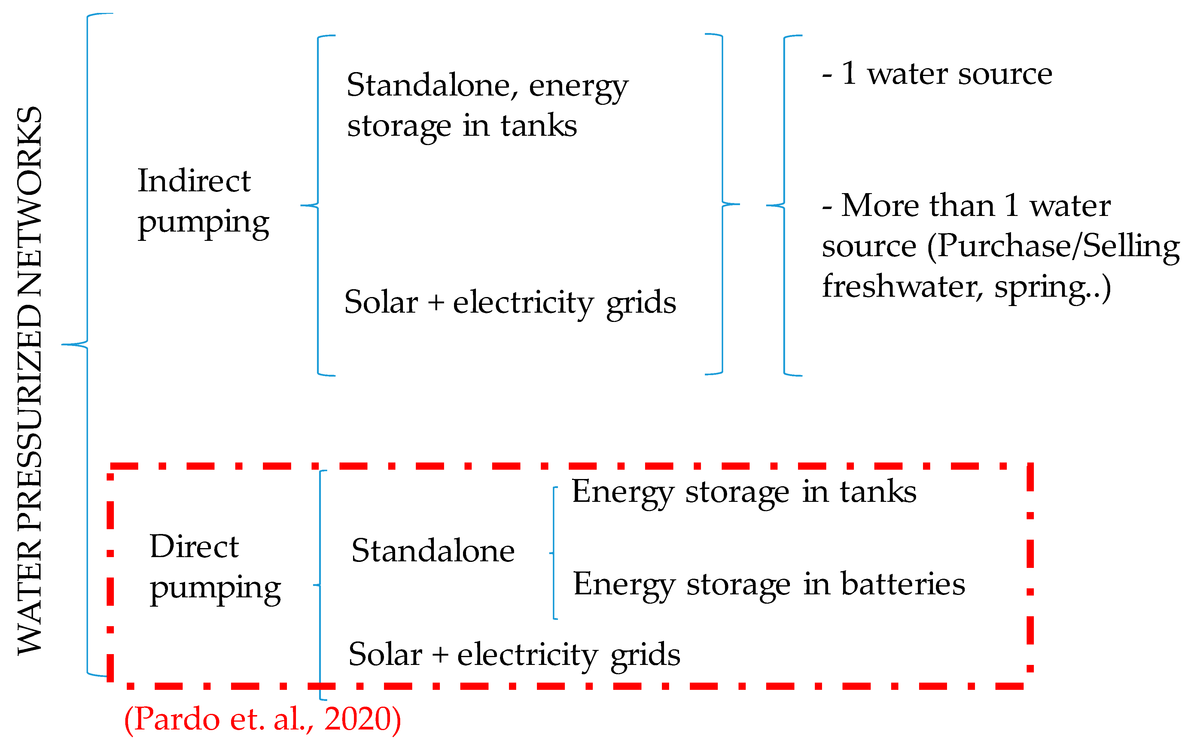
2.1. Types of Water Pressurized Distribution Networks

We present the cases found according to how we injected water into the system (Figure 1). Two options appeared: direct pumping (without head tanks) and indirect water supply (throughout the head tanks). We considered the first in [71], and we analyzed the second cases (indirect supply with head tanks as a guarantee for emergencies) found according to the municipality water precedence.

The first peculiarity is apparent considering the number of water resources, whether just one (groundwater, superficial water bodies, desalination, etc.) or several sources. The second involves acquiring/selling freshwater (irrigation communities or any alternative towns), thus solving the water scarcity problems in springs (a common situation in Southeast Spain [80]).

2.1.1. Use of PV Arrays in a Standalone System

If a WPN is converted into a standalone full PV supplied system, energy is stored in the head tanks. The PV modules must be dimensioned for the worst month (the month selected to size the system). In this month, the pump can operate enough hours so as to not endanger the guarantee of supply to the municipality. The indirect supply means not using batteries to save energy. Utility operators accumulate energy in a head tank with a great capacity to satisfy water demands. During the year, there may be periods with low values of solar irradiance, which involve low energy production. If the solar radiation data are available for a long period, it will be possible to check the highest number of days in which the radiation does not exceed the minimum necessary for the pumping station to extract groundwater, in order to have a real reference of the autonomy that the tank should have.

Equation (1) [71] serves to determine the volume accumulated to maintain supply at nights (${\forall }_{stored}$):

$${\forall }_{stored}\ge {\forall }_{cons}-{\forall }_{cons-irr}$$

(1)

where ${\forall }_{cons}$ is the city daily water demand and ${\forall }_{cons-irr}$ is the volume consumed when there is sunlight and the PV arrays are supplying electricity to the water pumps.

2.1.2. Use of PV Modules in a Hybrid System

This alternative delivers fresh water to the town by consuming energy produced by PV modules and taken from the grids. This is a favorable situation since it avoids a great deposit, however, it requires flexibility when determining the number of photovoltaic modules and the hours of operation supplied by PV modules. Thus, the manager must change the pumping hours to reach higher savings.

Another outstanding improvement of the mixed pumping is the phenomenon that, during summer, the peak values of energy costs (11:00 to 15:00) coincide with the higher solar radiation available. The cheapest energy costs are from 00:00 to 08:00, a period in which there will never be enough solar radiation for the pumps to handle. This means that solar pumping and grid-connected pumping complement each other, and in case power from the grid is needed, it will be there in the valley period (lowest costs).

2.1.3. Use of PV Modules in Several Source Supplies

Two options are available: the first is when the utility has the possibility of purchasing/selling fresh water to others, and when the second water source is a spring with high variability.

The first option is to connect the WPN to an irrigation network (fed by groundwater from aquifers) or linked to any alternative water source (remaining the opportunity of purchasing water). The utility manager must advise on the water provisions and cost of water throughout the day (and we do not handle the savings derived from the low-cost periods). Remarkably, to deal with the possibility of selling water to other users during the summer; other uses increase water expenditure (irrigation, urban consumption, etc.). The purchase of the excess volume can be a significant budgetary income that would maximize future savings.

The second option appears when we connect the WPN to a spring. In these communities, the major disadvantage is the unpredictable amount of water gathered from the spring, since they have substantial fluctuations throughout the year. Frequently, the absence of rainfall during autumn can cause water scarcity in winter and spring. If there is no alternative water resource connected to the grid network or the possibility of purchasing water, the sequence of a standalone pump providing water and spring is not workable.

2.2. Monthly and Yearly Variation in Energy Produced in PV Arrays

Many factors influence energy production in PV modules (latitude, temperature, tilt angle, azimuth, etc.). We dealt with the intensity of solar radiation as measured in the climatic station. Many investigations have presented the solar irradiation level as being the lowest in winter and the highest in summer [71,81,82]. As a result, the irradiation values in four months are far below the average value. This measurement accumulates the energy losses due to sun irradiance (soiling, dirt, and dust in solar modules, shading, orientation and tilt angle, air pollution, etc.). For instance, energy losses in dirt and dust range from around 2–50% [83], while shading ranges around 10–70% [84]. In our approach, we considered that PV cleaning maintenance is selected to avoid energy losses from dirt and dust and PV arrays are not affected by shading losses through trees, houses, or other bodies in proximity to PV modules. To reduce losses by temperature (8–15% in the module [85]), we will install spacers to allow 15–20 mm of space between PV modules to allow air circulation and cooling down the PV plant. Many investigations have proved the yearly average daily solar to increase over the years [86,87]. However, we assumed that the observed irradiance remained constant for the following years of analysis (this being a conservative hypothesis).

Water and energy demands are higher during summer and this period coincides with greater energy production. The utility manager must conduct a hydraulic test (considering the network details) to choose the most adverse month. The monthly water consumption (got measuring monthly water demands) is considered with a (K) parameter. In our analysis, we estimated that water consumption continues constantly for consecutive years. This is, again, a cautious hypothesis as Spain has displayed a decline in water expenditure in cities in recent years (−17% between 2000 and 2014) [88].

2.3. Life Cycle Cost of PV Modules

This method intends to give information to utility managers when they analyzed whether it is better to use batteries or tanks for energy storage or an intermediate mixed solution for several WPN. We consider here all the future costs and benefits in ‘present-day’ values. As the value of money changes with time, it would be unrealistic to add up the future costs as they stand. Future costs and benefits must be discounted to their equivalent value in today’s money [89], called their “net present value”. With these investments and future revenues, the objective function to maximize from the present time (tp) to the time $T^{*}$ can be expressed as the net present value (NPV) (Equation (2)):

$$NPV=-{\displaystyle \sum }{I}_0\cdot e^{-rt}-{{\displaystyle \int }}_0^{T^{*}}{S}_i\cdot e^{-r\cdot t}\cdot dt$$

(2)

where $I_0$ is the investment performed in year zero and $S_i$ is the monetary savings. We measured the benefits of installing a SPWS plant in every installation for a common lifespan (usually $T^{*}$ = 25 years).

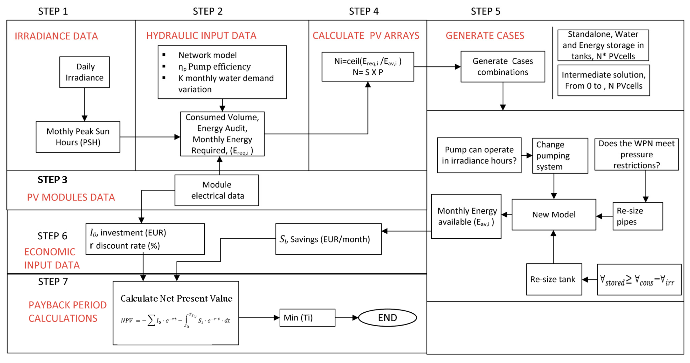
2.4. Calculation Process

Figure 2 reflects the computation process described by seven steps. First, we can retrieve the irradiance inputs (Step 1). With the daily solar period data from Step 1 and the network model (pumps, pipes, etc.), we can calculate the energy consumption and volume required (Step 2). We can obtain the PV modules data (Step 3) and with the results gathered in Step 2, we can calculate the number of PV panels, N (S modules in series and P modules in parallel). The new cases are described in (Step 5), considering potential requirements (new diameters for pipelines, new pumps, increase volume of the head tank, etc.) and can also determine the energy savings (Step 5) for each probable situation (standalone SPWS or hybrid system). The latest situation (the WPN operates by taking power from the electricity grids) incorporates many potential schemes, each of them with the installation of several PV modules. Likewise, in Step 5, we can assess the purchases for the cases mentioned before, and determine the net present value for every scheme in Step 6.

Step 1: Data recovery of the monthly energy available in the location.

Step 2: Calculation of the pumps monthly electric demands, the water consumption, and the worst month. This calculation requires Step 1 data and hydraulic data. The utility manager must estimate if the pump can elevate the total volume of water to the tank, if the dimensions of the pipeline are suitable, and if the tank size suffices the alternative procedure plan.

Step 3: PV modules data. We recovered the data from the PV modules selected for this analysis.

Step 4: Calculation of the number of PV arrays.

We calculated the minimum number of solar panels to produce more energy than the energy demanded by the WPN [51,71]. This resulted in a 12 × 1 vector that showed the number of modules for every month (the number of solar PV modules required being the greatest of these values). These numbers do not depend on the energy storage system and represent the upper limit for the hybrid case. If the SPWS can work as a standalone system, it makes little sense to work in a hybrid case.

Step 5: Generation of alternatives.

The first alternative was to convert the WPN as a standalone system accumulating energy in a head tank. Later, we created some combinations with a different number of PV modules (varying among the number of panels installed in parallel to allow connection) for the hybrid solution.

Step 6: Calculation of the economic input data.

We decided the investments because of the data proportioned in Step 3 and the economic accumulations for the alternatives outlined before (Step 5). In our method, we do not deal with the head tank or pipelines; these costs are included in every case. However, we incorporated new pump costs and increasing tank capacity. In the hybrid alternative, each combination requires different expenses (each combination involves a different number of PV modules) and savings (the more energy is produced, the lower the energy consumed in the grids).

Step 7: Calculation of the net present value for the alternatives.

The greatest net present value at the time ($T^{*}$; service life of the SPWS) is the most efficient option. This alternative was selected for implementation.

3. Case Study

3.1. Input Data

3.1.1. Hydraulic Data

The problem requires a hydraulic model to bring the water and energy consumed by the municipality (2000 inhabitants). These values depend on temperature, month, temperature, etc.

The hydraulic data required here are:

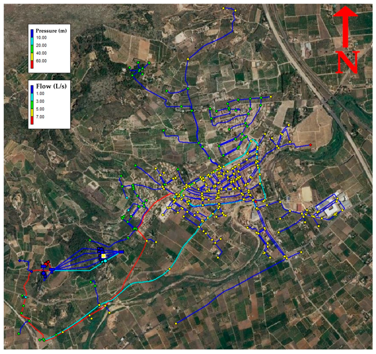
• The calibrated model is presented in Figure 3 (UTMX 754,387 and UTMY 4299526). We can simulate the hydraulic behavior of the WPN. This file must contain the information to perform hydraulic calculations without no error (elevation, base demands in nodes, roughness, diameter and lengths in pipes, pump curves, size of tanks, etc.). We propose Case 0 as the current state in which we supply pumps with electricity grids. The pumps start and stop as controlled by the water level in the tank. The method to carry out simulations is meant to suit the EPANET models for the water table depth (one model for each month) for Case 0.
• Pump ATURIAXRN6B (eight impellers). The curves of the pumps that show the head and pump efficiency variation with flow rates are depicted in Equations (3) and (4):

$$H\left(m\right)=-0.0561Q^2-1.0002Q+216.49 Q \left(\frac{l}{s}\right)$$

(3)

$${\mathsf{\eta }}_p(-)=-0.00006Q^2+0.0408Q+0.1618 Q \left(\frac{l}{s}\right)$$

(4)

• Water demand change per month (K). We calculate this variable by dividing each monthly water consumption into the average water demand. Their values are shown in

  Table 1. Water depth table, average temperature, and water consumption for each month.

  Month	1	2	3	4	5	6	7	8	9	10	11	12
  Water table depth (m)	52.76	51.79	49.44	58.13	58.21	57.17	56.27	55.35	57.84	57.95	57.63	59.08
  Volume (m3/day)	866	876	892	902	916	1007	1105	1047	956	891	840	830
  Average T (ª)	12.62	13.25	15.26	15.45	19.01	22.98	27.18	26.72	24.31	22.79	16.30	14.86
  K parameter	0.93	0.94	0.96	0.97	0.99	1.09	1.19	1.13	1.03	0.96	0.91	0.90

  .
• Consumption of the municipality: monthly volumes and “instant” flows (average flow every 30 min. This is necessary to calculate the average monthly consumption and daily patterns (Table 1).
• Water depths: Average of the dynamic level each month to calculate the pump head (Table 1).
• When the WPN operates as a SPWS, it requires pump SP-125-5-A (Grundfos). The curves of the pumps are shown Equations (5) and (6):

$$H\left(m\right)=-0.0417Q^2-0.3496Q+149.22 Q \left(\frac{l}{s}\right)$$

(5)

$${\mathsf{\eta }}_p(-)=-0.00098Q^2+0.06227Q+0.33794 Q \left(\frac{l}{s}\right)$$

(6)

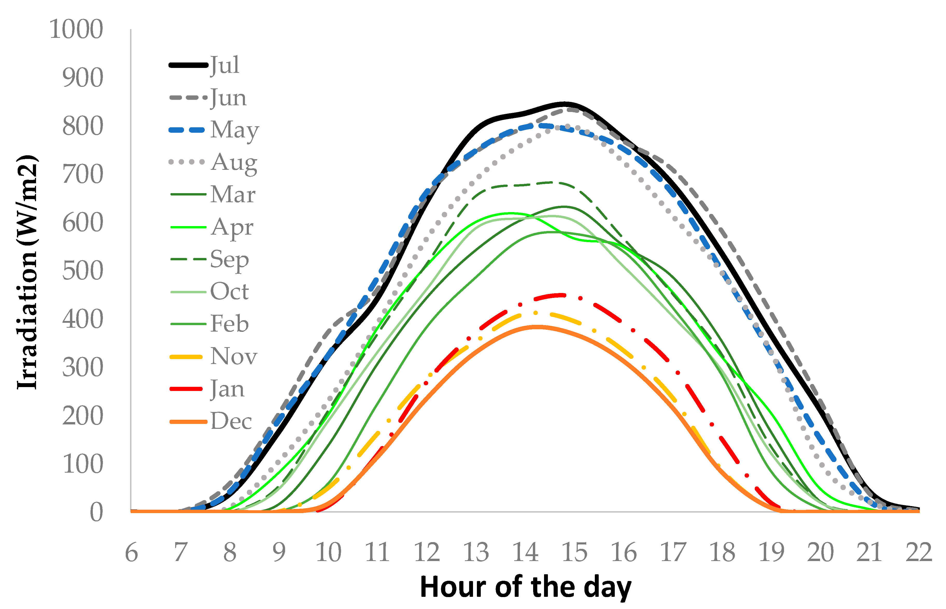
3.1.2. Irradiance Data

Solar radiation: The average radiation (W/m²) for each hour of the day, for each month of the year. This is essential to design the area of the solar park and to calculate the hours that the pump will work (and the frequency at which the inverter will work), depending on the month. We measured the irradiation data at the Sagra Station, which is located close to the WPN. The irradiation sensor was an SKU: 6450, and we integrated it into the Davis Pro 2 weather station. This station has been running since 7 November 2018, and we recovered data every 30 min (Figure 4). High irradiance months (July, June, May and August) can be seen in dark colors; the intermediate months (in green); and the low irradiance months (November, December and January) in warm colors. The peak sun hours (PSH) can be calculated from the irradiance data. The PSH ranges between 3.96 and 6.48 h in December and in July, respectively.

3.1.3. Economic Data

The economic data required to achieve the net present value are:

• Equivalent continuous discount rate (r = 2%).
• Investment (I0). We can calculate this amount for the option studied. PV modules, batteries, and pumps costs (service life 25, 5 and 7 years individually) and some other costs are displayed in

  Table 2. Costs for calculating investments.

  Components	Investment
  PV array	0.29 (EUR/Peak Power)
  Support structure	0.31 (EUR/Peak Power)
  Control system with safety cabinet	4252.67 (EUR)
  Assembly and commissioning	0.21 (EUR/Peak Power)
  Legalization process	1650 (EUR)
  Material transport	0.05 (EUR/Peak Power)
  Oversizing tank	100 (EUR/m3)
  New pump	12,900 EUR
  Battery	4330.58 EUR

  . These costs are identical for every option planned (to allow for a comparison).
• Economic savings (Si) in contrast to the present situation (Case 0). To determine energy expenditure costs, we have followed the Spanish tariff (which means determining power, energy, and reactive energy with hourly and seasonal variation). We calculated the hydraulics and the electricity bill.

The investment to install the PV panels (1.96 × 0.992 m²; an input data that depends on the PV panels selected), structure, legalization process, etc. and tank increase is depicted in Table 2. These numbers have been proportioned by a PV panel installer and a water utility in Spain. The modules were poly-crystalline Canadian Solar 330P (nominal maximum power 330 W, operating voltage 37.2 V, operating current 8.8 A, and open-circuit voltage 45.6 V), and the tilt angle was 40° and oriented to the south. The module efficiency was 19.67%, as declared by the manufacturer.

We retrieved the variable energy costs linked to the water distribution in the WPN at the zero-scenario. These costs have been calculated considering the 3.0 Tariff. This tariff covers three periods: the peak period extends for 4 h (prices are 0.111586 EUR/kWday and 0.112686 EUR/kWh); the plain period extends for 12 h (0.066952 EUR/kWday and 0.091485 EUR/kWh); and the low period extends for 8 h (0.044634 EUR/kWday and 0.064503 EUR/kWh). To further describe the reality, we included a 5.11% tax (direct electricity tax), a renting electricity meter rate (0.197377 EUR/day), and the value added tax (VAT) (21%, the general price in Spain).

3.2. Case Simulation

We present here the key cases that may appear in the town WPN (Case I, II, and III), while Case 0 represents the current state (electricity supplied by grids). We simulated the cases considering their monthly variation (we developed twelve hydraulic simulation models). In our approach, we did not consider the trackers (mechanical devices to move the modules). We computed the monthly energy consumption and production to confirm December as the most unfavorable month. This month had the lowest ratio between solar radiation and water needs, which coincides with earlier works [71].

When we used solar energy (Cases I, II, and III) in December, the low values of solar radiation involved means that the pump can work enough hours to supply the municipality (Figure 4). We should also select a pump that can provide water at a much higher head than the operating one, so that when pumping at a lower frequency, despite the lowering of the pumping curve, the pump can still satisfy the flow requirements. The model simulating the pumping conditions will depend on the hours when there is enough solar radiation for the pump to work. If there is an inverter, the power required at different frequencies can be calculated to have more hours of pumping.

3.2.1. The Current State, Case 0

We set up the WPN model of a small town (pumping with relation to the electrical grid) with the above-mentioned circumstances. The reservoir simulated an aquifer whose water level presents the average (dynamic) depth of that month. The supply conditions must keep the pumps operating from 00:00 to 08:00 h and as little as possible for the peak hours (from 11:00 to 15:00 in summer and from 19:00 to 23:00 in winter time). The simulation stage will correspond to the hours of the month (744, 720, and 672 for 31, 30, and 28 days, respectively).

3.2.2. Case I: Standalone Solar Water Pressurized Networks. Storage of Energy in the Head Tank

We calculated the daily water consumption for every month considering values ranging among 829.53 and 1103.351 m³/day in December and in July, respectively. If only solar pumping is accessible (no grid electricity), the reservoir should enhance its capacity by 725 m³ to feed the municipality during the night. Case I is presented in Figure 1 as several sources supplying water to the system and energy storage in tanks.

The pumping devices must deliver the whole volume of water in 4–7 h, which means higher flowrates (and head losses) than those expected when dimensioning this WPN. Arrangements such as choosing a new pump, re-dimensioning pipeline diameters, or widening the tank size were not the mean target of this study, which was to evaluate the new WPN that could run isolated from the electricity grids. If only solar pumping is available (Case I), the cost of the electric bill will be zero after the conversion. We dimensioned the SPWS and found that this town requires 18 × 16 PV arrays (18 modules in series and 16 modules in parallel).

3.2.3. Case II: Hybrid System Supplied by Solar and Grid Electricity Consumption

Case II is the intermediate case fed by the electricity grids and PV arrays. We calculated pumping costs in “cheap”, “medium”, and “expensive” periods (values dependent on the season and the hour of the day). We entered these values in electricity bill templates to calculate the cost of the monthly electricity bill.

In this scenario, the economic savings only affected the energy consumption term (other terms such as power installed remained constant). With the second strains, we calculated the energy savings for several PV array areas installed in 18 × 12, 18 × 10, 18 × 8, and 8 × 6 modules (considering the intermediate cases as those obtained with the elimination of modules in parallel). Case II was presented in Figure 1 as several sources supplying water to the system and a hybrid system supplying energy to the WPN.

3.2.4. Case III: Standalone Solar Water Pressurized Networks Selling the Surplus of Energy

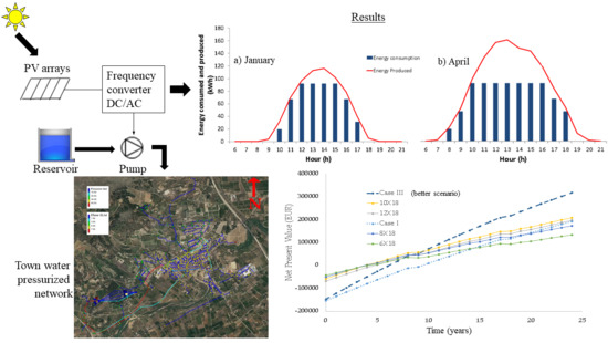
This case was similar to Case I (standalone solar system, 18 × 16 modules, a new pump, and a 725 m³ increase in tank capacity). We developed this scenario to understand how much energy-savings can arise if we can sell this excess of energy to the electricity distribution company. In Spain, the approval of this operation scheme is much slower than the Case I scheme. We propose this alternative to quantify this effect.

4. Results

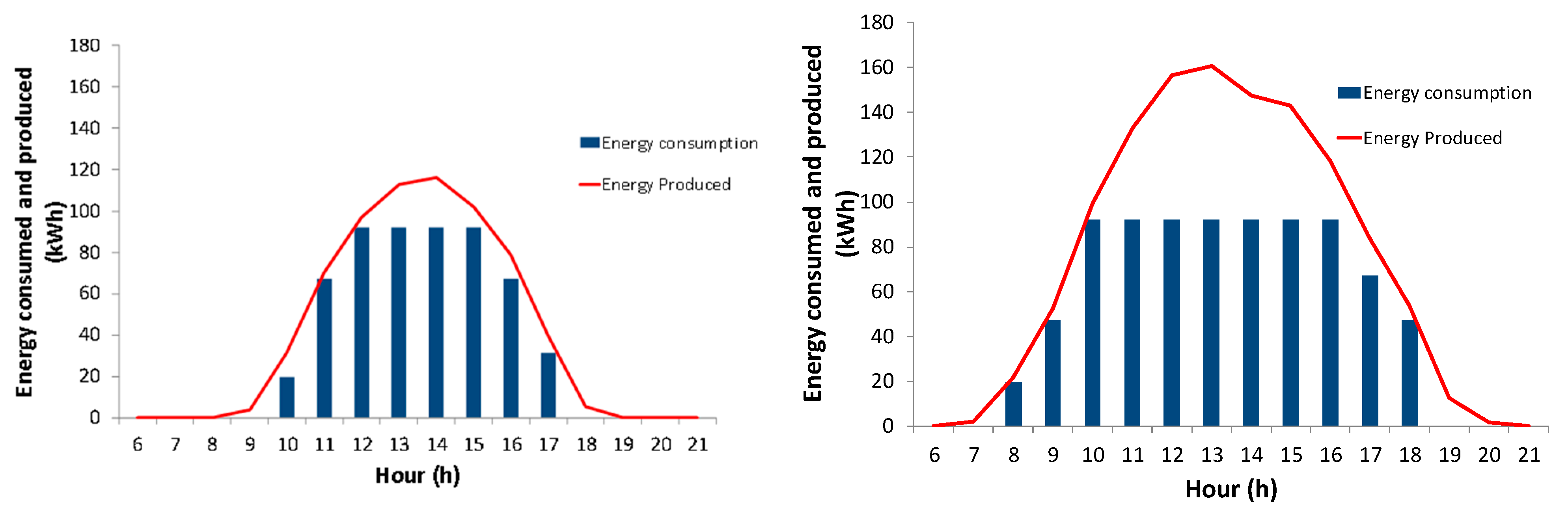
4.1. Monthly Energy Consumption

We used UAEnergy [79] to calculate the monthly water and energy consumption in our town, and these values are depicted in

Table 3. Volume, electricity consumption, and monthly costs in the town (Case 0).

		Case 0 and II		Cases I and III
Month	V Cons(m3)	Energy Pump (kWh/Month)	Electricity Consumption (kWh/Month)	Energy Pump (kWh/Month)	Electricity Consumption (kWh/Month)
Jan	26,815.34	4326.10	6010.18	5010.13	8692.32
Feb	24,548.24	3792.40	5421.72	3957.85	7590.35
Mar	27,570.35	4186.42	5947.15	5261.56	8799.37
Apr	27,004.40	4100.16	6000.56	4633.22	8362.75
May	28,331.28	4464.27	6354.66	5266.42	8263.84
Jun	30,229.41	5024.67	7000.89	6035.93	10,502.33
Jul	34,203.82	5842.62	8008.63	6383.65	11,151.94
Aug	31,447.66	5751.03	8054.08	6489.61	10,483.40
Sep	27,679.97	5348.40	7396.64	5502.19	9574.05
Oct	27,581.85	5266.46	7038.41	5537.66	9282.07
Nov	25,186.92	4604.14	6222.95	4703.62	8420.10
Dec	25,715.41	4625.13	6269.17	5173.66	8471.47

. UAEnergy reported the volume and energy consumed. The pump-efficiency relationship converts this energy consumed into electricity consumption.

When we produce an SPWS, the consumed volume is equal to the consumed volume in Case 0 (to allow comparison and to represent the water supply appropriately). However, the energy consumption (and electricity) are higher as a consequence of larger head losses and flow rates [90]. The most unfavorable month is December, as it had the minimum value of the ratio PSH/(V consumed).

4.2. Calculation of the Yearly Electricity Cost

With these data, we calculated the economic energy consumption (

Table 4. Economic electric consumption (EUR) in the town.

Month	Case 0	Case I	Case II 18 × 12	Case II 18 × 10	Case II 18 × 8	Case II 18 × 6	Case III
Jan	1512.32	0	292.54	315.23	315.23	450.92	−337.38
Feb	1427.10	0	315.23	292.54	292.54	393.66	−370.83
Mar	1572.53	0	307.67	315.23	315.23	315.23	−618.24
Apr	1527.44	0	315.23	307.67	307.67	307.67	−691.72
May	1597.31	0	307.67	315.23	315.23	315.23	−789.28
Jun	1631.39	0	315.23	307.67	307.67	337.56	−646.64
Jul	1797.60	0	315.23	315.23	315.23	408.90	−692.52
Aug	1774.27	0	307.67	315.23	315.23	436.11	−704.79
Sep	1646.58	0	315.23	307.67	307.67	463.22	−551.18
Oct	1722.51	0	307.67	315.23	328.75	520.15	−381.70
Nov	1575.15	0	315.23	307.67	332.58	498.57	−292.52
Dec	1587.88	0	80.84	315.23	362.74	524.35	−258.93

). The Case I savings coincided with Case 0 consumption (the utility does not pay for electricity). Case II savings were lower than in Case I as they considered the electricity taken from electricity grids in comparison with the Case 0 use. In short, Case II (18 × 12 = 216 modules) involves savings in January of 1512.32–292.54 = 1219.78 EUR.

4.3. Sale of Surplus Energy

To calculate the surplus energy (Table 4), the energy available and the energy consumed must be known. The latter can be calculated in two steps: calculation of the available energy and energy consumption. In Figure 4, we show the hourly irradiance values obtained per month and the energy demanded by the pumps (Figure 5). As we have the energy produced (red line, Figure 5) and consumed (blue rectangles), we can obtain the surplus energy by subtracting them. As an example, we show these values in January and April.

The excess of energy takes place when there is energy available, but cannot be supplied as it fills the tank of water (

Table 5. Monthly energy surplus (kW h/month).

Month	Energy Production (kWh/Month)	Energy Consumption (kWh/Month)	Energy Surplus (kWh/Month)
Jan	12,758.31	8692.32	4065.98
Feb	12,022.02	7590.35	4431.67
Mar	15,935.36	8799.37	7135.99
Apr	16,301.94	8362.75	7939.19
May	17,269.45	8263.84	9005.61
Jun	17,948.85	10,502.33	7446.51
Jul	19,099.92	11,151.94	7947.98
Aug	18,565.52	10,483.40	8082.12
Sep	15,977.04	9574.05	6402.99
Oct	13,832.53	9282.07	4550.46
Nov	11,995.81	8420.10	3575.71
Dec	11,680.01	8471.47	3208.54

). This condition demands a recent monthly run of the hydraulic EPANET model. We exported the tank level, the outlet tank flow rate, and injecting flow rate. We should encounter the intervals at which the tank is full and deduct the inlet and outlet flow rates to obtain the surplus flow. If we divide this excess of flow by the pump flow rate for the frequency at which the pump is performing, we can identify the hours when the pump is not functioning and the excess energy. The sum of the monthly values and the monthly energy surplus returns the total energy.

The fact of being able to inject the electricity surplus into the grids involves maintaining the utility connected to the grid. This also involves having a minimum of power installed (and according to this, an additional cost). Please note, electricity grid consumption should be avoided on cloudy days as the WPN demands electricity in the “expensive” hours.

4.4. Calculation of the Investments and Savings

In Case I, the PV modules, the new pump and increasing tank capacity (by 725 m³ as stated before) represent the investments to address in year 0. The peak power required is 0.330 ∗ 288 = 95.04 kW. Using the cost data depicted in Table 2, and assuming that a new pump is purchased every nine years, we can calculate the investment for Case I as shown in Equation (7) (

Table 6. Investment I₀ (EUR) for the analyzed cases.

		Case II
Components	Case I and III	18 × 12	18 × 10	18 × 8	18 × 6
PV array	27,561.60	20671.2	17226	13,780.80	10,335.60
Support structure	29,462.40	22,096.80	18414	14,731.20	11,048.40
Control with safety cabinet	4252.67	4252.67	4252.67	4252.67	4252.67
Assembly and commissioning	19,958.4	14,968.80	12474	9979.20	7484.4
Legalization process	1650	1650	1650	1650	1650
Material transport	4752	3564	2970	2376	1782
Oversizing tank	72,570.79
New pump	32,675.01	32,675.01	32,675.01	32,675.01	32,675.01
Battery		17,905.67	17,905.67	17,905.67	17,905.67
TOTAL	192,882.87	117,784.15	107,567.35	97,350.55	87,133.75

).

$$\begin{array}{l}{I}_0{}^{*}=(0.29+0.31+0.21+0.05)\ast 95,040+1650+4252.67+725\ast 100+\\ 12,900\ast (1+{\mathrm{e}}^{-0.02\ast 9}+{\mathrm{e}}^{-0.02\ast 18})=192,882.87 \mathrm{EUR}\end{array}$$

(7)

In Case II, we calculated the investment in an analogous manner, but the costs of increasing the tank were not considered and we purchased a battery every five years. For Case II with 18 × 12 modules, the investment results in Equation (8) (Table 6).

$$\begin{array}{l}{I}_0{}^{*}=(0.29+0.31+0.21+0.05)\ast 330\ast 18\ast 12+1650+4252.67+725\ast 100+\\ 12,900\ast (1+{\mathrm{e}}^{-0.02\ast 9}+{\mathrm{e}}^{-0.02\ast 18})+4330.58\ast (1+{\mathrm{e}}^{-0.02\ast 5}+{\mathrm{e}}^{-0.02\ast 10}+{\mathrm{e}}^{-0.02\ast 15}+{\mathrm{e}}^{-0.02\ast 20})=\\ 117,784.15 \mathrm{EUR}\end{array}$$

(8)

Electricity consumption in Case 0 is energy savings for Cases I and III (standalone system). In Case II, we connected the WPN to the grids and the PV arrays produced power during sunlight. Therefore, savings influence the energy term of those three already mentioned in the tariff for calculating the electricity bill (other terms such as power remaining constant), as shown in

Table 7. Energy savings S_i (EUR) for the analyzed cases.

		Case II
Month	Case I	18 × 12	18 × 10	18 × 8	18 × 6	Case III
January	1512.32	1512.32	1219.78	1197.09	1197.09	1512.32
February	1427.10	1427.1	1111.87	1134.56	1134.56	1427.10
March	1572.53	1572.53	1264.86	1257.30	1257.30	1572.53
April	1527.44	1527.44	1212.21	1219.77	1219.77	1527.44
May	1597.31	1597.31	1289.64	1282.08	1282.08	1597.31
June	1631.39	1631.39	1316.16	1323.72	1323.72	1631.39
July	1797.60	1797.6	1482.37	1482.37	1482.37	1797.60
August	1774.27	1774.27	1466.60	1459.04	1459.04	1774.27
September	1646.58	1646.58	1331.35	1338.91	1338.91	1646.58
October	1722.51	1722.51	1414.84	1407.28	1393.76	1722.51
November	1575.15	1575.15	1259.92	1267.48	1242.57	1575.15
December	1587.88	1587.88	1507.04	1272.65	1225.14	1587.88
Power fixed term	0					−415.2
Electricity Sale	0	0	0	0	0	6750.93
TOTAL	19,372.08	15,876.66	15,642.27	155,556.33	14,400.51	25,707.81

. Case III differed from Case I in that the WPN was connected to the electricity grids (to sell the surplus) and the company was forced to pay a fixed term, referring to the power that can be taken. This is the reason that there is a new cost, which is shown as a negative saving.

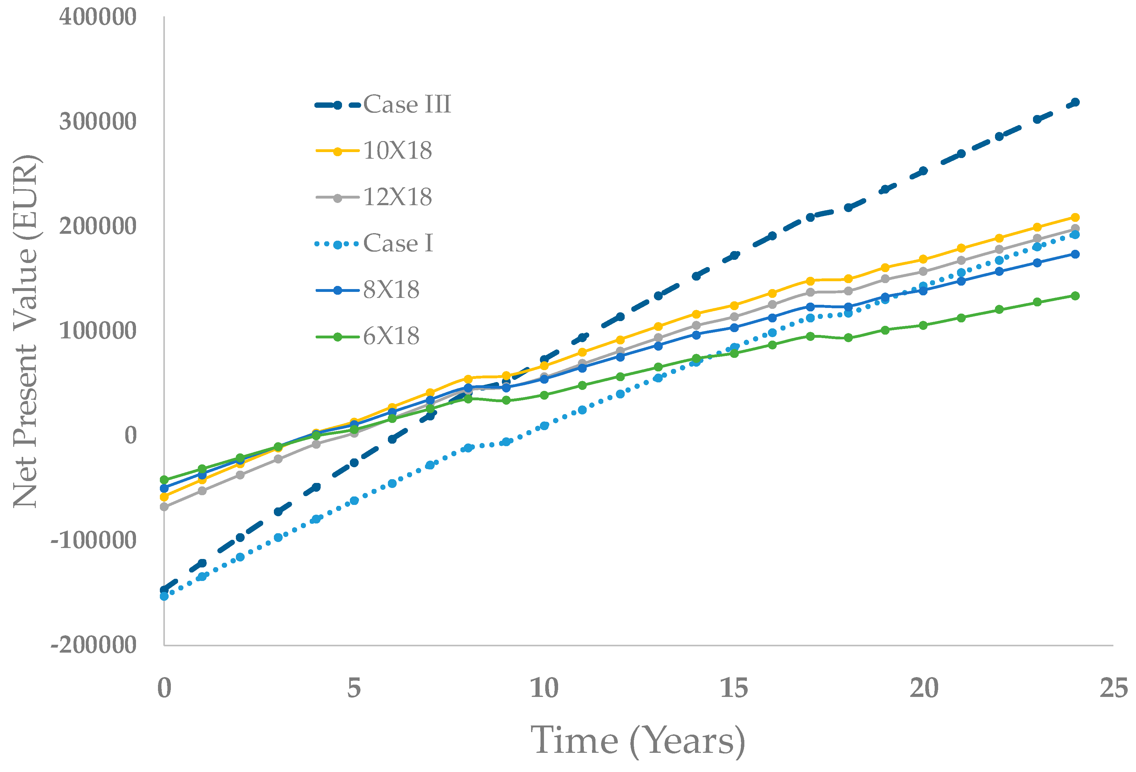
4.5. Life Cycle Cost Calculations

The payback period ([60]) for Cases I and III returned the numerical values of 11.10 and 8.13 years, respectively. We obtained other values for the huge (although finite) possibility of installing an area between 0 and 288 modules (559.96 m²) in Case II.

However, the net present value for year 25 (PV installation lifespan) indicates that Case III results in the best alternative for the whole lifespan of the SPWS. We may find that some misleading data would have appeared, if the payback period was considered as an indicator. Case II (18 × 6 modules) resulted in the worst combination for the life cycle cost analysis (as it had very low future revenues) and had a lower payback period. In Figure 6, the axis of the year ranges from now to the maximum expected lifespan of 25 years. We can observe that when the number of modules increases in Case II, higher savings result in greater net present values. The best option was Case III, as the savings were higher than any of the other alternatives.

5. Discussion

The water consumption ranged from 25,715.41 m³/month in December and 34,203.82 m³/month in July. The energy production per single PV array was 1743.10 kWh/day (the peak value in July was 2139.33 kWh/day and the lowest value was 1308.25 kWh/day in December). We obtained these numbers by multiplying the PSH by the maximum module power. The average peak sun hours were 5.28, while the maximum and the minimum were 6.48 (July) and 3.96 h (December).

Using renewable energies is more convenient than conventional electricity supply through grids. The utility is saving energy (109,593.99 kWh per year; Table 3) and emissions to the environment (considering each country energy mix). These saved credit carbons can very much contribute to avoiding climate change.

In our approach, we pretended to deal with the key uncertainties parameters found here, the variability of water consumption and solar irradiance. We solved the first considering a monthly analysis with different water consumption (based on historical values of the municipality consumption) and a different water level of the aquifer. Thereafter, we measured the solar irradiance for the last two years at Sagra Station to obtain the actual values of irradiation, as we already considered the shading effect on the panels in our approach. We also considered that the PV installation received proper maintenance with frequent PV cleaning. This approach requires a WPN model to perform the calculations.

6. Conclusions

This work helps decision-makers to select the most efficient alternative for a real urban WPN from an economic standpoint. We considered two alternatives: converting the WPN into a standalone photovoltaic system or into a hybrid (grid + solar) system. To avoid misleading, we studied irradiation and energy expenditure fluctuation. Peak values of energy expenditure (in summer) coincided with peak values of energy production. We confirmed that the worst month was December because energy production reduces much of that energy consumption.

This manuscript presents a method that allows for the adaptation of any urban WPN into a standalone SPWS with energy storage in tanks, and into a hybrid system. We practiced this method in a real municipality, and discovered that energy production varied more than energy consumption in this WPN. This means that December is the most adverse month as it bears the lowest irradiance and thus the lowest energy production.

The tank alternative (Case I and III) is more energy-hungry than the others, as the pumping devices should fill the head tank in a quick time (those with irradiation needed to provide the pumps’ work). Case III bears no surprise as it illustrates that when the electric company purchases the excess energy, it produces greater revenues in the SPWS lifespan following 25 years. This case study proved that we reimbursed the investment of 11.10 − 8.13 = 2.97 years (

Table 8. The payback period and net present value for the cases analyzed.

	Investments (EUR)	Savings (EUR)	Payback Period (Years)	Net Present Value (EUR)
Case I	192,882.87	19,372.08	11.10	192,056.97
Case II 18 × 12	117,784.15	15,876.66	8.03	197,698.61
Case II 18 × 10	107,567.35	15,642.27	7.26	208,741.96
Case II 18 × 8	97,350.55	15,556.33	7.21	173,283.95
Case II 18 × 6	87,133.75	14,400.51	7.71	133,893.43
Case III	192,882.87	25,707.81	8.13	317,953.36

) previously in Case III. Therefore, we can handle these numbers to encourage WPN to sell excess energy, without being worried about the delay in getting the SPWS certified to add electricity to the grids. Case III is the best choice from the economic standpoint investigation presented here.

Many service managers promote the hybrid alternative (Case II) (although a worse solution than Case III, Table 8) to avoid problems supplying water to municipalities (as a guarantee for supply). These solutions (fluctuating from 108 to 216 modules) feature lower economic savings (as the service is even rewarding to the electrical company). Selecting the best Case II solution (10 × 18 modules) involves wasting 317,953.36 − 208,741.96 = 109,211.4 EUR in the next 25 years.

We have shown that the payback period is not a good indicator in this case (with high variability in savings). The lowest payback period (Case II 18 × 8 modules) resulted in the second-worst combination for the life cycle cost analysis.

We could further develop this procedure considering the forecasted values of irradiance (including external parameters that can be of bias). To represent reality, future municipality conditions can vary corresponding to estimated values of water demands and population growth. In this municipality, the consumption trend is slightly down from the latest data. In Case III, if consumption was to fall, the utility could sell more energy and could expect higher revenues.

References

1. UNESCO-WWAP Facts and Figures from the United Nations World Water Development Report 4 (WWDR4); UNESCO: Paris, France, 2012.
2. UN World Water Development Report; 2019.
3. Burek, P.; Satoh, Y.; Fischer, G.; Kahil, M.T.; Scherzer, A.; Tramberend, S.; Nava, L.F.; Wada, Y.; Eisner, S.; Flörke, M.; et al. Water futures and solution-fast track initiative. In IIASA Working Paper; IIASA: Laxenburg, Austria, 2016. [Google Scholar]
4. Ram, M.; Bogdanov, D.; Aghahosseini, A.; Oyewo, S.; Gulagi, A.; Child, M.; Fell, H.-J.; Breyer, C. Global Energy System Based on 100% Renewable Energy—Power Sector; Lappeenranta University of Technology and Energy Watch Group: Lappeenranta, Finland, 2017. [Google Scholar]
5. IEA. World Energy Outlook 2019; IEA: París, France, 2019. [Google Scholar]
6. IEA. Water-Energy Nexus; IEA: París, France, 2017. [Google Scholar]
7. Bijl, D.L.; Bogaart, P.W.; Kram, T.; de Vries, B.J.M.; van Vuuren, D.P. Long-term water demand for electricity, industry and households. Environ. Sci. Policy 2016, 55, 75–86. [Google Scholar] [CrossRef]
8. Hardy, L.; Garrido, A.; Juana, L. Evaluation of Spain’s Water-Energy Nexus. Int. J. Water Resour. Dev. 2012, 28, 151–170. [Google Scholar] [CrossRef] [Green Version]
9. IDAE. Consumo Energético en el Sector del Agua; IDAE: Madrid, Spain, 2010. [Google Scholar]
10. Jäger-Waldau, A. PV Status Report 2019, EUR 29938 EN; Publications Office of the European Union: Luxembourg, 2019. [Google Scholar]
11. Goodrich, A.C.; Powell, D.M.; James, T.L.; Woodhouse, M.; Buonassisi, T. Assessing the drivers of regional trends in solar photovoltaic manufacturing. Energy Environ. Sci. 2013, 6, 2811–2821. [Google Scholar] [CrossRef] [Green Version]
12. REN 21 Renewables Now. Renewables Global Status Report 2019; REN21: Paris, France, 2019; ISBN 9783981891140. [Google Scholar]
13. Gorjian, S.; Zadeh, B.N.; Eltrop, L.; Shamshiri, R.R.; Amanlou, Y. Solar photovoltaic power generation in Iran: Development, policies, and barriers. Renew. Sustain. Energy Rev. 2019, 106, 110–123. [Google Scholar] [CrossRef]
14. Chazarra-Zapata, J.; Molina-Martínez, J.M.; Cruz, F.-J.P.D.L.; Parras-Burgos, D.; Ruíz Canales, A. How to Reduce the Carbon Footprint of an Irrigation Community in the South-East of Spain by Use of Solar Energy. Energies 2020, 13, 2848. [Google Scholar] [CrossRef]
15. Cimorelli, L.; Covelli, C.; Molino, B.; Pianese, D. Optimal Regulation of Pumping Station in Water Distribution Networks Using Constant and Variable Speed Pumps: A Technical and Economical Comparison. Energies 2020, 13, 2530. [Google Scholar] [CrossRef]
16. EC. Communication from the Commission to the European Parliament, the European Council, the European Economic and Social Committee, the Committee of the Regions and the European Investment Bank. A Clean Planet for all A European Strategic Long-Term Vision for; EC: Brussels, Belgium, 2018. [Google Scholar]
17. Closas, A.; Rap, E. Solar-based groundwater pumping for irrigation: Sustainability, policies, and limitations. Energy Policy 2017, 104, 33–37. [Google Scholar] [CrossRef]
18. Mincotur. Precio neto de la electricidad para uso doméstico y uso industrial Euros/kWh. Available online: https://www.mincotur.gob.es/es-ES/IndicadoresyEstadisticas/DatosEstadisticos/IV.Energíayemisiones/IV_12.pdf (accessed on 20 September 2004).
19. Muhsen, D.H.; Khatib, T.; Abdulabbas, T.E. Sizing of a standalone photovoltaic water pumping system using hybrid multi-criteria decision making methods. Sol. Energy 2018, 159, 1003–1015. [Google Scholar] [CrossRef]
20. Khatib, T.; Ibrahim, I.A.; Mohamed, A. A review on sizing methodologies of photovoltaic array and storage battery in a standalone photovoltaic system. Energy Convers. Manag. 2016, 120, 430–448. [Google Scholar] [CrossRef]
21. AlSkaif, T.; Dev, S.; Visser, L.; Hossari, M.; van Sark, W. A systematic analysis of meteorological variables for PV output power estimation. Renew. Energy 2020, 153, 12–22. [Google Scholar] [CrossRef]
22. González, L.G.; Chacon, R.; Delgado, B.; Benavides, D.; Espinoza, J. Study of Energy Compensation Techniques in Photovoltaic Solar Systems with the Use of Supercapacitors in Low-Voltage Networks. Energies 2020, 13, 3755. [Google Scholar] [CrossRef]
23. Järvelä, M.; Valkealahti, S. Operation of a PV Power Plant during Overpower Events Caused by the Cloud Enhancement Phenomenon. Energies 2020, 13, 2185. [Google Scholar] [CrossRef]
24. Corizzo, R.; Ceci, M.; Japkowicz, N. Anomaly Detection and Repair for Accurate Predictions in Geo-distributed Big Data. Big Data Res. 2019, 16, 18–35. [Google Scholar] [CrossRef]
25. Behera, M.K.; Majumder, I.; Nayak, N. Solar photovoltaic power forecasting using optimized modified extreme learning machine technique. Eng. Sci. Technol. Int. J. 2018, 21, 428–438. [Google Scholar] [CrossRef]
26. Sobri, S.; Koohi-Kamali, S.; Rahim, N.A. Solar photovoltaic generation forecasting methods: A review. Energy Convers. Manag. 2018, 156, 459–497. [Google Scholar] [CrossRef]
27. Ceci, M.; Corizzo, R.; Malerba, D.; Rashkovska, A. Spatial autocorrelation and entropy for renewable energy forecasting. Data Min. Knowl. Discov. 2019, 33, 698–729. [Google Scholar] [CrossRef]
28. Jane, R.; Parker, G.; Vaucher, G.; Berman, M. Characterizing meteorological forecast impact on microgrid optimization performance and design. Energies 2020, 13, 577. [Google Scholar] [CrossRef] [Green Version]
29. Bakelli, Y.; Arab, A.H.; Azoui, B. Optimal sizing of photovoltaic pumping system with water tank storage using LPSP concept. Sol. Energy 2011, 85, 288–294. [Google Scholar] [CrossRef]
30. Mwanza, M.; Kaoma, M.; Bowa, C.K.; Çetin, N.S.; Ülgen, K. The potential of solar energy for sustainable water resource development and averting national social burden in rural areas of Zambia. Period. Eng. Nat. Sci. 2017, 5. [Google Scholar] [CrossRef] [Green Version]
31. Arab, A.H.; Chenlo, F.; Mukadam, K.; Balenzategui, J.L. Performance of PV water pumping systems. Renew. Energy 1999, 18, 191–204. [Google Scholar] [CrossRef]
32. Narvarte, L.; Almeida, R.H.; Carrêlo, I.B.; Rodríguez, L.; Carrasco, L.M.; Martinez-Moreno, F. On the number of PV modules in series for large-power irrigation systems. Energy Convers. Manag. 2019, 186, 516–525. [Google Scholar] [CrossRef]
33. Aliyu, M.; Hassan, G.; Said, S.A.; Siddiqui, M.U.; Alawami, A.T.; Elamin, I.M. A review of solar-powered water pumping systems. Renew. Sustain. Energy Rev. 2018, 87, 61–76. [Google Scholar] [CrossRef]
34. Pande, P.C.; Singh, A.K.; Ansari, S.; Vyas, S.K.; Dave, B.K. Design development and testing of a solar PV pump based drip system for orchards. Renew. Energy 2003, 28, 385–396. [Google Scholar] [CrossRef]
35. Linssen, J.; Stenzel, P.; Fleer, J. Techno-economic analysis of photovoltaic battery systems and the influence of different consumer load profiles. Appl. Energy 2017, 185, 2019–2025. [Google Scholar] [CrossRef]
36. Beck, T.; Kondziella, H.; Huard, G.; Bruckner, T. Assessing the influence of the temporal resolution of electrical load and PV generation profiles on self-consumption and sizing of PV-battery systems. Appl. Energy 2016. [Google Scholar] [CrossRef]
37. Tsuanyo, D.; Azoumah, Y.; Aussel, D.; Neveu, P. Modeling and optimization of batteryless hybrid PV (photovoltaic)/Diesel systems for off-grid applications. Energy 2015. [Google Scholar] [CrossRef]
38. Yu, C.; Khoo, Y.S.; Chai, J.; Han, S.; Yao, J. Optimal orientation and tilt angle for maximizing in-plane solar irradiation for PV applications in Japan. Sustainability 2019, 11, 2016. [Google Scholar] [CrossRef] [Green Version]
39. Hailu, G.; Fung, A.S. Optimum Tilt Angle and Orientation of Photovoltaic Thermal System for Application in Greater Toronto Area, Canada. Sustainability 2019, 11, 6443. [Google Scholar] [CrossRef] [Green Version]
40. Kacira, M.; Simsek, M.; Babur, Y.; Demirkol, S. Determining optimum tilt angles and orientations of photovoltaic panels in Sanliurfa, Turkey. Renew. Energy 2004, 29, 1265–1275. [Google Scholar] [CrossRef]
41. Khatib, T.; Mohamed, A.; Sopian, K. Optimization of a PV/wind micro-grid for rural housing electrification using a hybrid iterative/genetic algorithm: Case study of Kuala Terengganu, Malaysia. Energy Build. 2012, 47, 321–331. [Google Scholar] [CrossRef]
42. Narvarte, L.; Fernández-Ramos, J.; Martínez-Moreno, F.; Carrasco, L.M.; Almeida, R.H.; Carrêlo, I.B. Solutions for adapting photovoltaics to large power irrigation systems for agriculture. Sustain. Energy Technol. Assess. 2018, 29, 119–130. [Google Scholar] [CrossRef] [Green Version]
43. Díaz-Dorado, E.; Suárez-García, A.; Carrillo, C.; Cidrás, J. Influence of the shadows in photovoltaic systems with different configurations of bypass diodes. In Proceedings of the SPEEDAM 2010—International Symposium on Power Electronics, Electrical Drives, Automation and Motion, Pisa, Italy, 14–16 June 2010. [Google Scholar]
44. Rydh, C.J.; Sandén, B.A. Energy analysis of batteries in photovoltaic systems. Part I: Performance and energy requirements. Energy Convers. Manag. 2005, 46, 1957–1979. [Google Scholar] [CrossRef]
45. Moharram, K.A.; Abd-Elhady, M.S.; Kandil, H.A.; El-Sherif, H. Influence of cleaning using water and surfactants on the performance of photovoltaic panels. Energy Convers. Manag. 2013, 68, 266–272. [Google Scholar] [CrossRef]
46. Wagner, L. Overview of Energy Storage Technologies. In Future Energy Improved, Sustainable and Clean Options for our Planet; Elsevier: Amsterdam, The Netherlands, 2013; pp. 613–631. [Google Scholar] [CrossRef]
47. Jossen, A.; Garche, J.; Sauer, D.U. Operation conditions of batteries in PV applications. Sol. Energy 2004, 76, 759–769. [Google Scholar] [CrossRef]
48. Bendary, A.F.; Ismail, M.M. Battery charge management for hybrid PV/wind/fuel cell with storage battery. Proc. Energy Procedia 2019. [Google Scholar] [CrossRef]
49. Mulder, G.; Six, D.; Claessens, B.; Broes, T.; Omar, N.; Mierlo, J. Van The dimensioning of PV-battery systems depending on the incentive and selling price conditions. Appl. Energy 2013, 111, 1126–1135. [Google Scholar] [CrossRef]
50. Jadhav, S.; Devdas, N.; Nisar, S.; Bajpai, V. Bidirectional DC-DC converter in Solar PV System for Battery Charging Application. In Proceedings of the 2018 International Conference on Smart City and Emerging Technology, ICSCET 2018, Mumbai, India, 5 January 2018; Institute of Electrical and Electronics Engineers Inc.: Mumbai, India, 2018. [Google Scholar]
51. Pardo, M.Á.; Juárez, J.M.; García-Márquez, D. Energy consumption optimization in irrigation networks supplied by a standalone direct pumping photovoltaic system. Sustainability 2018, 10, 4203. [Google Scholar] [CrossRef] [Green Version]
52. Mérida García, A.; Fernández García, I.; Camacho Poyato, E.; MontesinosBarrios, P.; Rodríguez Díaz, J.A. Coupling irrigation scheduling with solar energy production in a smart irrigation management system. J. Clean. Prod. 2018, 175, 670–682. [Google Scholar] [CrossRef]
53. Üçtug, F.G.; Azapagic, A. Environmental impacts of small-scale hybrid energy systems: Coupling solar photovoltaics and lithium-ion batteries. Sci. Total Environ. 2018, 643, 1579–1589. [Google Scholar] [CrossRef] [Green Version]
54. Betka, A.; Attali, A. Optimization of a photovoltaic pumping system based on the optimal control theory. Sol. Energy 2010, 84, 1273–1283. [Google Scholar] [CrossRef]
55. Elkholy, M.M.; Fathy, A. Optimization of a PV fed water pumping system without storage based on teaching-learning-based optimization algorithm and artificial neural network. Sol. Energy 2016, 139, 199–212. [Google Scholar] [CrossRef]
56. Mohanty, A.; Ray, P.K.; Viswavandya, M.; Mohanty, S.; Mohanty, P.P. Experimental analysis of a standalone solar photo voltaic cell for improved power quality. Optik (Stuttgart) 2018, 171, 876–885. [Google Scholar] [CrossRef]
57. Ru, Y.; Kleissl, J.; Martinez, S. Storage size determination for grid-connected photovoltaic systems. IEEE Trans. Sustain. Energy 2013, 4, 68–81. [Google Scholar] [CrossRef] [Green Version]
58. Peng, J.; Lu, L.; Yang, H. Review on life cycle assessment of energy payback and greenhouse gas emission of solar photovoltaic systems. Renew. Sustain. Energy Rev. 2013, 19, 255–274. [Google Scholar] [CrossRef]
59. Todde, G.; Murgia, L.; Carrelo, I.; Hogan, R.; Pazzona, A.; Ledda, L.; Narvarte, L. Embodied Energy and Environmental Impact of Large-Power Stand-Alone Photovoltaic Irrigation Systems. Energies 2018, 11, 2110. [Google Scholar] [CrossRef] [Green Version]
60. Pardo, M.A.; Manzano, J.; Valdés-Abellán, J.; Cobacho, R. Standalone direct pumping photovoltaic system or energy storage in batteries for supplying irrigation networks. Cost analysis. Sci. Total Environ. 2019, 673, 821–830. [Google Scholar] [CrossRef] [Green Version]
61. Kaldellis, J.K.; Zafirakis, D.; Kondili, E. Energy pay-back period analysis of stand-alone photovoltaic systems. Renew. Energy 2010, 35, 1444–1454. [Google Scholar] [CrossRef]
62. Skoczek, A.; Sample, T.; Dunlop, E.D. The results of performance measurements of field-aged crystalline silicon photovoltaic modules. Prog. Photovolt. Res. Appl. 2009, 17, 227–240. [Google Scholar] [CrossRef]
63. Li, C.H.; Zhu, X.J.; Cao, G.Y.; Sui, S.; Hu, M.R. Dynamic modeling and sizing optimization of stand-alone photovoltaic power systems using hybrid energy storage technology. Renew. Energy 2009, 34, 815–826. [Google Scholar] [CrossRef]
64. Sani Hassan, A.; Cipcigan, L.; Jenkins, N. Optimal battery storage operation for PV systems with tariff incentives. Appl. Energy 2017, 203, 422–441. [Google Scholar] [CrossRef]
65. Spiers, D. Chapter IIB-2—Batteries in PV Systems. In Practical Handbook of Photovoltaics, 2nd ed.; McEvoy, A., Markvart, T., Castañer, L.B.T.-P.H., Eds.; Academic Press: Boston, MA, USA, 2012; pp. 721–776. ISBN 978-0-12-385934-1. [Google Scholar]
66. Ghoneim, A.A. Design optimization of photovoltaic powered water pumping systems. Energy Convers. Manag. 2006, 47, 1449–1463. [Google Scholar] [CrossRef]
67. Hugues, K.W.; Daniel Chowdhury, S.P. An African solution for water and electricity supply, using a standalone photovoltaic based Quasi Z Source Inverter. In Proceedings of the IEEE PES PowerAfrica Conference, PowerAfrica 2016, Livingstone, Zambia, 28 June–3 July 2016. [Google Scholar]
68. Todde, G.; Murgia, L.; Deligios, P.A.; Hogan, R.; Carrelo, I.; Moreira, M.; Pazzona, A.; Ledda, L.; Narvarte, L. Energy and environmental performances of hybrid photovoltaic irrigation systems in Mediterranean intensive and super-intensive olive orchards. Sci. Total Environ. 2019, 651, 2514–2523. [Google Scholar] [CrossRef]
69. Wong, J.; Lim, Y.S.; Tang, J.H.; Morris, E. Grid-connected photovoltaic system in Malaysia: A review on voltage issues. Renew. Sustain. Energy Rev. 2014, 29, 535–545. [Google Scholar] [CrossRef]
70. Tsagas, I. Spain Approves ‘Sun Tax’, Discrimiates Against Solar PV. Renew. Energy World 2015. [Google Scholar]
71. Pardo, M.Á.; Cobacho, R.; Bañón, L. Standalone Photovoltaic Direct Pumping in Urban Water Pressurized Networks with Energy Storage in Tanks or Batteries. Sustainability 2020, 12, 738. [Google Scholar] [CrossRef] [Green Version]
72. Reddy, P.P.K.K.; Reddy, J.N. Photovoltaic energy conversion system for water pumping application. Int. J. Emerg. Trends Electr. Electron. 2014, 10, 22–29. [Google Scholar]
73. Vindel, J.M.; Polo, J.; Zarzalejo, L.F. Modeling monthly mean variation of the solar global irradiation. J. Atmos. Solar-Terrestrial Phys. 2015, 122, 108–118. [Google Scholar] [CrossRef]
74. Rehman, S.; Bader, M.A.; Al-Moallem, S.A. Cost of solar energy generated using PV panels. Renew. Sustain. Energy Rev. 2007, 11, 1843–1857. [Google Scholar] [CrossRef]
75. Hamidat, A.; Benyoucef, B. Systematic procedures for sizing photovoltaic pumping system, using water tank storage. Energy Policy 2009, 37, 1489–1501. [Google Scholar] [CrossRef]
76. Nabila, L.; Khaldi, F.; Aksas, M. Design of photo voltaic pumping system using water tank storage for a remote area in Algeria. In Proceedings of the IREC 2014—5th International Renewable Energy Congress, Hammamet, Tunisia, 25–27 March 2014. [Google Scholar]
77. Gómez, E.; Cabrera, E.; Balaguer, M.; Soriano, J. Direct and Indirect Water Supply: An Energy Assessment. Procedia Eng. 2015, 119, 1088–1097. [Google Scholar] [CrossRef] [Green Version]
78. Rossman, L.A. EPANET 2: Users Manual; Environmental Protection Agency (US): Washington, DC, USA, 2000.
79. Pardo, M.A.; Riquelme, A.; Melgarejo, J. A tool for calculating energy audits in water pressurized networks. AIMS Environ. Sci. 2019, 6, 94–108. [Google Scholar]
80. Valdes-Abellan, J.; Pardo, M.A.; Jodar-Abellan, A.; Pla, C.; Fernandez-Mejuto, M. Climate change impact on karstic aquifer hydrodynamics in southern Europe semi-arid region using the KAGIS model. Sci. Total Environ. 2020, 723, 138110. [Google Scholar] [CrossRef]
81. Osinowo, A.A.; Okogbue, E.C.; Ogungbenro, S.B.; Fashanu, O. Analysis of Global Solar Irradiance over Climatic Zones in Nigeria for Solar Energy Applications. J. Sol. Energy 2015, 2015, 1–9. [Google Scholar] [CrossRef] [Green Version]
82. Bou-Rabee, M.A.; Sulaiman, S.A. On seasonal variation of solar irradiation in Kuwait. Int. J. Renew. Energy Res. 2015, 5, 367–372. [Google Scholar]
83. Maghami, M.R.; Hizam, H.; Gomes, C.; Radzi, M.A.; Rezadad, M.I.; Hajighorbani, S. Power loss due to soiling on solar panel: A review. Renew. Sustain. Energy Rev. 2016, 59, 1307–1316. [Google Scholar] [CrossRef] [Green Version]
84. Hajighorbani, S.; Radzi, M.A.M.; Ab Kadir, M.Z.A.; Shafie, S.; Khanaki, R.; Maghami, M.R. Evaluation of fuzzy logic subsets effects on maximum power point tracking for photovoltaic system. Int. J. Photoenergy 2014, 2014, 719126. [Google Scholar] [CrossRef]
85. Vaillon, R.; Dupré, O.; Cal, R.B.; Calaf, M. Pathways for mitigating thermal losses in solar photovoltaics. Sci. Rep. 2018, 8, 1–9. [Google Scholar]
86. Lima, F.J.L.D.; Martins, F.R.; Costa, R.S.; Gonçalves, A.R.; dos Santos, A.P.P.; Pereira, E.B. The seasonal variability and trends for the surface solar irradiation in northeastern region of Brazil. Sustain. Energy Technol. Assess. 2019, 35, 335–346. [Google Scholar] [CrossRef]
87. Zhou, Y.; Meng, X.; Belle, J.H.; Zhang, H.; Kennedy, C.; Al-Hamdan, M.Z.; Wang, J.; Liu, Y. Compilation and spatio-temporal analysis of publicly available total solar and UV irradiance data in the contiguous United States. Environ. Pollut. 2019, 253, 130–140. [Google Scholar] [CrossRef]
88. Sauri, D. The decline of water consumption in Spanish cities: Structural and contingent factors. Int. J. Water Resour. Dev. 2019. [Google Scholar] [CrossRef]
89. Kleiner, Y.; Rajani, B. Comprehensive review of structural deterioration of water mains: Statistical models. Urban Water 2001, 3, 131–150. [Google Scholar] [CrossRef] [Green Version]
90. Pardo, M.Á.; Riquelme, A.J.; Jodar-Abellan, A.; Melgarejo, J. Water and Energy Demand Management in Pressurized Irrigation Networks. Water 2020, 12, 1878. [Google Scholar] [CrossRef]
Figure 1. Cases found when planning to convert a water pressurized network into a PV supplied service.
Energies 13 04013 g001
Figure 2. Workflow for the process to calculate the net present value of the alternatives.
Energies 13 04013 g002
Figure 3. Town water pressurized network.
Energies 13 04013 g003
Figure 4. Monthly average irradiation (W/m2).
Energies 13 04013 g004
Figure 5. The energy produced and consumed in January (left) and in April (right).
Energies 13 04013 g005
Figure 6. The Net Present Value for the alternatives.
Energies 13 04013 g006