Abstract
The paper features an examination of the link between the behaviour of oil prices and DowJones Index in a nonlinear autoregressive distributed lag nonlinear autoregressive distributed lag (NARDL) framework. The attraction of NARDL is that it represents the simplest method available of modelling combined short- and long-run asymmetries. The bounds testing framework adopted means that it can be applied to stationary and non-stationary time series vectors, or combinations of both. The data comprise a monthly West Texas Intermediate (WTI) crude oil series from Federal Reserve Bank of St Louis (FRED), commencing in January 2000 and terminating in February 2019, and a corresponding monthly DOW JONES index adjusted-price series obtained from Yahoo Finance. Both series are adjusted for monthly USA CPI values to create real series. The results of the analysis suggest that movements in the lagged real levels of monthly WTI crude oil prices have very significant effects on the behaviour of the DOW JONES Index. They also suggest that negative movements have larger impacts than positive movements in WTI prices, and that long-term multiplier effects take about 9 to 12 months to take effect.
1. Introduction
The paper explores the link between oil prices and Dow Jones Index in a nonlinear autoregressive distributed lag (NARDL) framework. Shin et al. [1] introduce short- and long-run nonlinearities via positive and negative partial sum decompositions of the explanatory variables. This model, as developed by [1], has a number of advantages. These include the capability of being estimated by OLS, and the use of bounds-testing to make reliable long-run inference. Bounds testing does not require the integration orders of the variables to be the same. In traditional cointegration analysis, all the variables would have to be non-stationary I(1).
The analysis is undertaken using the R library package ‘nardl’ by Zagdoudhi [2]. This package also uses R code to implement the bounds tests confidence intervals on the dynamic multipliers, as suggested by Philips [3], using code that he made available (the ‘nardl’ library uses the R package ‘pss’ which Philips [4] placed on ‘Github’ to undertake this http://andyphilips.github.io/pss/).
The paper explores the links between oil price changes and movements in the Dow Jones Index, using the latest developments in nonlinear time-series modelling techniques, in a framework that is capable of capturing both short-run and long-run effects. Shin et al. [1] draw attention to the vast literature that has developed around the concept of cointegration and the analysis of non-stationarity, which commenced with Dickey and Fuller [5], Engle and Granger [6], Johannsen [7], Phillips and Hansen [8], and Kwiatkowski et al. [9], which represent major landmarks.
Park and Phillips [10] explore nonlinear econometric analysis for non-stationary time series. They demonstrate that the spatial features of a time series can play a significant role in the relevant asymptotics. A further generalisation of this approach to encompass a time trend and stationary regressors, and multiple I(1) regressors, is provided by Chang et al. [11].
Bierens and Martin [12] developed a vector ECM with time-varying properties. The Johansen framework is a special case. Park and Hahn [13] followed the approach of Engle and Granger [6] and proposed a cointegrating regression with time-varying parameters. They conceded that this form of cointegration is quite restrictive, as only the coefficients are assumed to be time-dependent.
The relationship between oil price changes and GDP in a non-cointegration framework, has been explored by Hamilton [14], who reported strong evidence of nonlinearity, and suggested that oil price increases have a greater impact than oil price decreases.
A considerable literature, developed since the mid 1990s, considered non-stationarity and nonlinearity jointly. Three regime-switching models have influence: threshold ECM associated with Balke and Fomby [15], Markov-switching ECM of Psaradakis et al. [16], and smooth transition regression ECM developed by Kapetanios et al. [17].
The approach reflects the view that simple linear adjustment processes may be too limited. Shin et al. [1] note that there is not a great deal of work on nonlinear cointegration. One exception is provided by Schorderet [18,19], who proposed a bivariate asymmetric cointegrating regression of unemployment on output, in which output is decomposed into partial sum processes of positive and negative changes.
Granger and Yoon [20] proposed the concept of ‘hidden cointegration’ that involved defining the cointegrating relationship between positive and negative components of variables. They point out that variables are cointegrated because they respond to shocks displaying common stochastic trends. Granger and Yoon [20], p. 5 query what the implications would be if they respond differently to positive and negative shocks. They suggest that there may be cointegration between non-stationary components of a data series, which they refer to as being ‘hidden cointegration’. Standard cointegration is a special case of hidden cointegration, a simple example of nonlinear cointegration.
Shin et al. [1] extend the work in this area, and provide a dynamic framework that is both simple and flexible, nonlinear, and capable of simultaneously and coherently modelling asymmetries. These are present in both the underlying long-run relationship and in dynamic adjustment. They derive the dynamic ECM associated with asymmetric long-run cointegrating regression to the nonlinear autoregressive distributed lag (NARDL).
They follow Pesaran et al. [21] and use a bounds testing approach to test for a stable long-run relationship. They also derive asymmetric cumulative dynamic multipliers that permit the display of the asymmetric adjustment patterns following positive and negative shocks to the explanatory variables.
Prior to the development of the flexible approach suggested by Shin et al. [1], there had been a few other studies that employed a NARDL framework. Van Treeck [22] used a NARDL model to analyse asymmetric wealth effects on US consumption.
In this paper, we apply a NARDL analysis of cointegration between the inflation-adjusted levels of the Dow Jones Index and the West Texas Intermediate Crude oil price series. We use the CPI for All Urban Consumers: All Items (CPIAUCSL) as a measure of inflation. In the process we provide a validation and application of the nonlinear autoregressive distributed lag NARDL framework as developed by Shin et al. [1] in relation to this topic.
2. The Links between Oil Prices and Stock Markets
There does not seem to be agreement amongst economists about the relationship between the price of oil and stock markets. Kling [23] suggested oil price increases are associated with stock market declines. By contrast, Chen et al. [24] suggested there is no relationship between asset prices and oil price changes, while Jones and Kaul [25] suggest the relationship between oil price changes and aggregate stock returns is stable and negative. Huang et al. [26] explored changes in oil price futures and stock returns, and found no indications of a negative relationship. Wei [27] suggested that the 1972–1974 oil price shock cannot be linked to the 1974 US stock price decline.
Kilian and Vigfusson [28] critiqued various approaches to the study of asymmetries in the relationship between the oil prices and US real economic activity, and concluded that asymmetric effects of oil price innovations on domestic real activity deserved further exploration.
Kilian and Park [29] suggest the reaction of the US real stock returns to a change in oil prices differs according to whether it is a demand- or supply-driven shock in oil. They use a structural VAR model of US stock market shocks to demand and supply shocks in oil. They suggest that changes in stock prices are more likely to reflect shocks to aggregate demand for industrial commodities, or shocks to precautionary demand for oil, that reflect oil supply uncertainty shortfall, as opposed to shocks to production of crude oil.
However, one drawback of using a standard VAR approach using differenced series is that it loses any information that may be captured in relationships between the levels of the series, as revealed by cointegration. Kilian and Park [29] criticised modelling approaches that assume that changes in the oil price are exogenous to the stock market. One of the attractions of the NARDL approach is that it reveals differences in the responses to positive and negative changes, and also how these change in the short and longer term.
The adoption of the bounds test also means that it can capture relationships between both stationary and non-stationary variables, as explained in the next sub-section.
3. Econometric Model—The Nardl Approach
Shin et al. [1] developed NARDL by considering an asymmetric long-run regression:
where and are scalar I(1) variables, and is decomposed as where and are partial sum processes of positive and negative changes in
The above provides modelling asymmetric cointegration with partial sum decompositions. Schorderet [19] defines a stationary linear combination of the partial sum components:
If is stationary, then and are ‘asymmetrically cointegrated’. The standard linear (symmetric) cointegration is a special case of (4), obtained only if and . Shin et al. [1] consider the case where the following restriction holds: In expression (4), this implies that and .
Shin et al. [1] use this foundation to propose the nonlinear ARDL (p,q) model:
where is a vector of multiple regressors, , is the autoregressive parameter, and are the asymmetric distributed lag parameters, and is an process with zero mean and constant variance, . Shin et al. [1] consider is decomposed into and around zero, distinguishing between positive and negative changes in rate of growth of .
They follow Pesaran et al. [21] and write (5) in the error correction form as:
where for for for , and is the nonlinear ECM, where and are the associated asymmetric long-run parameters.
In order to deal with non-zero contemporaneous correlation between regressors and residuals in (6), Shin et al. [1] propose the following reduced form data generation process for
where with a positive definite covariance matrix. In terms of their focus on conditional modelling, they express in terms of as:
where is uncorrelated with , by construction. If we substitute (8) into (6) and rearrange, we obtain a nonlinear conditional ECM:
where and for
Equation (9) corrects for weak endogeneity of non-stationary explanatory variables, and the choice of lag structure free the model from any residual correlation. The model explains both long and short-run asymmetries and, as it is linear in all parameters, can be estimated by OLS.
The approach above is implemented in the R library package ‘nardl’, developed by Zagdoudhi [2] and in the R library package ‘pss’ by Jordan and Philips [30]. The ‘pssbounds’ function from the latter package is used in the ‘nardl’ package.
4. Results of the Analysis
4.1. Preliminary Analysis
The sample data set consists of the monthly series of the CPI for All Urban Consumers: All Items (CPIAUCSL), which is used as a measure of inflation. This series is taken from the Federal Reserve Bank of St Louis (FRED) database. The series is seasonally adjusted, and has a base of 1982–1984. We also use the monthly West Texas Intermediate (WTI) crude oil series from FRED (Crude Oil Prices: West Texas Intermediate (WTI)—Cushing, Oklahoma (DCOILWTICO)). (FRED data available at: https://fred.stlouisfed.org/).
The data series commences in January 2000 and terminates in February 2019. The monthly Dow Jones index adjusted-price series are obtained from Yahoo Finance. We inflation-adjust the oil price and Dow Jones series, and use the lagged real oil price series in the analysis. This results in a data set with 228 observations, or 227 when we run NARDL estimation with the lag of the real WTI price. (Yahoo finance datasets used to be directly accessible on the web but this feature was removed. Yahoo finance data can still be accessed indirectly via an Application Programming Interface (API). We used the R library ’quantmod’ by Ryan and Ulrich [31]).
Summary statistics are presented in Table 1. The mean value of the real monthly level of the Dow Jones index series is 62.18, and the mean value of the real lagged monthly level of the WTI crude oil index is 0.286. The two series in Figure 1 show they appear to trend together. Both appear to be suitable for NARDL analysis in that they do not embody uniformly positive or negative changes.

Table 1.
Summary statistics.
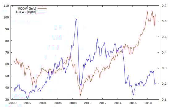
Figure 1.
Plots of real values of Dow Jones Index and West Texas Intermediate (WTI) Crude Oil Index.
The QQ plots in Figure 2 show both series have fat tails, and are not Gaussian. This is not surprising, as we would expect the levels of the series to be non-stationary.
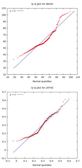
Figure 2.
QQ plots of real values of the Dow Jones Index and WTI Crude Oil Index.
This is confirmed by Augmented Dickey Fuller (ADF) test results shown in Table 2. The tests, undertaken with a constant, and constant and a trend, fail to reject the null hypothesis of a unit root, as indicated by the asymptotic probability values in parentheses.
Table 2.
Augmented Dickey-Fuller (ADF) Tests.
Table 3 presents simple Engle–Granger tests of cointegration between the two series, using models with a constant, and a constant and trend. At first glance, results in Table 3 appear promising, in that all the coefficients estimated in the Engle–Granger two-step cointegration test procedure appear to be highly significant, whether the equation includes constant, or constant and time trend. However, unit root tests on the residuals from the two regressions both fail to reject the unit root null hypothesis, which suggests that the regression results are spurious.
Table 3.
Engle–Granger tests of cointegration.
A potential issue is that the series spans the period of the Global Financial Crisis (GFC), usually attributed to 2007–2009, and this raises the issue of potential structural breaks (We are grateful to an anonymous reviewer for drawing our attention to this issue.). We used the R package ‘strucchange’ to undertake Bai-Perron [32] tests for existence of structural breaks in the base series, RDOW and LRWTI, the real monthly levels of the DOW index and the lagged real levels of the WTI oil index. The four suggested breakpoints, after OLS regression of Real Dow in levels on lagged Real TWI levels, were in 2005 December, 2008 October, 2013 February, and 2016 January. We estimated Engle–Granger cointegration tests for the two base series in these four sub-periods, but the results showed no evidence of cointegration. A potential issue is that the full sample series comprise 228 monthly observations, so that the sub-periods examined are relatively short.
As a further check on whether the base series exhibited trending behaviour, we estimated the Hurst Exponent [33], (H), for the two series. The Hurst exponent for RDOW was 0.975263 and that for LRWTI was 1.01246. A value of H in the range 0.5–1.0 indicates long-term positive autocorrelation, suggestive of long-term memory and trending behaviour. A value in the range 0–0.5 indicates a tendency to switch between high and low values in adjacent pairs, suggesting mean-reversing behaviour. Finally, a value of H of around 0.5 is suggestive of Brownian motion, or a series with no memory, which follows a random walk. The H value for both series suggests trending behaviour. Therefore, we are confident in using cointegration tests to explore whether they trend together.
A further benefit, of the Shin et al. [1] NARDL approach is that it provides a simple and flexible nonlinear dynamic framework capable of simultaneously and coherently modelling asymmetries, both in the underlying long-run relationship and in the patterns of dynamic adjustment. They claim that the approach makes four contributions: the first is the derivation of a dynamic error correction representation associated with the asymmetric long-run cointegrating regression, resulting in the nonlinear autoregressive distributed lag (NARDL) model. The second is that, in the process, they use a bounds-testing procedure for existence of stable long-run relationship, irrespective of whether the underlying regressors are I(0), I(1), or are mutually cointegrated.
Their third contribution is that they derive asymmetric cumulative dynamic multipliers that permit the tracing out of the asymmetric adjustment patterns following positive and negative shocks to the explanatory variables. Their approach is sufficiently flexible to accommodate four combinations of long- and short-run asymmetries.
By means of Monte Carlo experiments, they validate their estimation and inference framework, and reveal little estimation bias and high power in test statistics. They also compute p-values for cointegration tests and confidence intervals for the dynamic multipliers by a non-parametric bootstrap. Thus, their approach is sufficiently general to permit its application to our two series, and will be valid whether or not the two series are cointegrated.
4.2. Nardl Analysis
We applied the R package ‘nardl’ by Zaghdoudi [2] to implement the estimation procedures for the relationship between the real monthly level of the Dow Jones Index RDOW and the lagged real monthly level of Texas West Intermediate crude oil LRWTI using four lags.
The results of estimation in Table 4 suggest the NARDL model successfully captures asymmetries in the responses of the real level of the Dow Jones index to changes in the real levels of lagged TWI crude oil prices. The responses to lagged negative changes are stronger than to lagged positive changes. This is apparent in values of long-run coefficients presented in the right-hand side of Table 4, in which the coefficient on the lagged positive change in TWI crude oil (LRTWI_p_1) is −40.24, while the coefficient on the lagged negative change in TWI crude oil (LRTWI_n_1) is approximately −70.50, or almost double the amount.
Table 4.
Nonlinear autoregressive distributed lag (NARDL) analysis.
The adjusted R-squared for the fitted model is 0.06617, and the F statistic for the model is highly significant. The Jarque-Bera (JB) test rejects the hypothesis that the residuals conform to a Gaussian distribution, but the Lagrange Multiplier (LM) test finds no evidence of serial correlation, while the ARCH test shows no presence of autoregressive conditional heteroscedasticity.
Figure 3 plots the CUSUM test of the residuals, which reveals that, as the model progresses beyond 160 observations of the total sample of 226 monthly values, the residuals are on the red borderline boundary at the 5% level, which suggests they are becoming borderline non-stationary. The simple Engle–Granger test of cointegration rejected the null of cointegration between the two series.
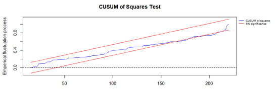
Figure 3.
CUSUM of squares test.
Thus, the NARDL specification, as used in this paper, can detect evidence in support of cointegration in circumstances in which the simple Engle–Granger approach might fail to do so.
Figure 4 plots the impact of the Dynamic Multiplier of positive and negative changes in real LTWI. The blue line in Figure 4 captures the impact of positive changes and the red line that of negative changes. The difference between the two is depicted by the broken line. It can be seen in Figure 4 that it takes about 12 to 13 months for the multipliers to work through their effects until a relatively stable impact is achieved. Falls in oil prices appear to have a larger impact on the Dow Jones Index than do increases in oil prices. The difference in the impacts appears to be at its greatest 9–12 months after it occurs, according to the evidence in Figure 4.
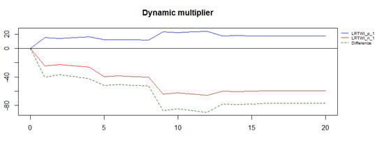
Figure 4.
Dynamic multiplier.
The results in this paper suggest that downward movements in oil prices have larger negative impacts on the Dow Jones Index than do upward movements. The results can be contrasted with a recent study by Jiang et al. [34], which uses a structural VAR to decompose oil price changes into oil supply shocks, global demand shocks, and oil specific demand shocks. However, their VAR analysis is all in differences. They impose restrictions on the VAR model, appealing to two prior models. The first model is a variant of the model advanced by Kilian [35].
The second model is a parsimonious version of Caldara, Cavallo, and Iacoviello [36] that facilitates joint identification of both oil supply and demand elasticities. Jiang et al. [34] argue that these three different shocks should have different effects on equity markets. They claim to be able to earn excess returns on portfolios constructed on the basis of their modelling, which is not consistent with the existence of time-varying risk premia. However, to identify their models, they need to make restrictive assumptions and do not include the information captured in the levels of their series.
Our results suggest that price decreases have a larger impact than price increases, but are not based upon assumptions made re the state of supply and demand in the relevant markets.
We would suggest that the NARDL framework, as used in this paper, has the merit of including both levels and differences of the relevant series, and that the bounds testing framework applied means that it can accommodate I(0) and I(1) sequences of variables, or combinations of both.
5. Conclusions
The coefficients reported in Table 4 suggest that both increases and decreases, or positive and negative movements in the price of oil, are both associated with Dow Jones Index declines, but that negative movements have larger effects. The exploration of these effects is a topic of future research.
Author Contributions
The authors contributed equally in all respects. All authors have read and agreed to the published version of the manuscript.
Funding
This research received no external funding.
Acknowledgments
The authors thank the reviewers for very helpful comments and suggestions, and Hashem Pesaran for insightful discussions.
Conflicts of Interest
The authors declare no conflict of interest.
References
- Shin, Y.; Yu, B.; Greenwood-Nimmo, M. Modelling asymmetric cointegration and dynamic multipliers in a nonlinear ARDL framework. In The Festschrift in Honor of Peter Schmidt.: Econometric Methods and Applications; Horrace, W., Sickles, R., Eds.; Springer: New York, NY, USA, 2014; pp. 281–314. [Google Scholar]
- Zaghdoudi, T. nardl: Nonlinear Cointegrating Autoregressive Distributed Lag Model; R Package Version 0.1.5; 2018; Available online: https://CRAN.R-project.org/package=nardl (accessed on 12 December 2019).
- Philips, A.Q. Have Your Cake and Eat It Too? Cointegration and dynamic inference from Autoregressive Distributed Lag Models. Am. J. Political Sci. 2018, 62, 230–244. [Google Scholar] [CrossRef]
- Philips, A.Q. pss: Perform Bounds Test for Cointegration and Perform Dynamic Simulations; R Package Version 0.1.3.9000; 2016; Available online: http://andyphilips.github.io/pssbounds/ (accessed on 12 December 2019).
- Dickey, D.A.; Fuller, W.A. Distribution of the estimators for autoregressive time series with a unit root. J. Am. Stat. Assoc. 1979, 74, 427–431. [Google Scholar]
- Engle, R.F.; Granger, C.W.J. Co-integration and error correction: Representation, estimation and testing. Econometrica 1987, 55, 251–276. [Google Scholar] [CrossRef]
- Johansen, S. Statistical analysis of cointegration vectors. J. Econ. Dyn. Control 1988, 12, 231–254. [Google Scholar] [CrossRef]
- Phillips, P.C.B.; Hansen, B. Statistical inference in instrumental variables regression with I(1) processes. Rev. Econ. Stud. 1990, 57, 99–125. [Google Scholar] [CrossRef]
- Kwiatkowski, D.; Phillips, P.C.B.; Schmidt, P.; Shin, Y. Testing the null hypothesis of stationarity against the alternative of a unit root. J. Econom. 1992, 54, 159–178. [Google Scholar] [CrossRef]
- Park, J.Y.; Phillips, P.C.B. Nonlinear regressions with integrated time series. Econometrica 2001, 69, 117–161. [Google Scholar] [CrossRef]
- Chang, Y.; Park, J.Y.; Phillips, P.C.B. Nonlinear econometric models with cointegrated and deterministically trending regressors. Econom. J. 2001, 4, 1–36. [Google Scholar] [CrossRef]
- Beirens, H.J.; Martins, L.F. Time-varying cointegration. Econom. Theory 2010, 26, 1453–1490. [Google Scholar] [CrossRef]
- Park, J.Y.; Hahn, S.B. Cointegrating regressions with time-varying coefficients. Econom. Theory 1999, 15, 664–703. [Google Scholar] [CrossRef]
- Hamilton, J.D. What is an oil shock? J. Econom. 2003, 113, 363–398. [Google Scholar] [CrossRef]
- Balke, N.S.; Fomby, T.B. Threshold cointegration. Int. Econ. Rev. 1997, 38, 627–645. [Google Scholar] [CrossRef]
- Psaradakis, Z.; Sola, M.; Spagnolo, F. On Markov error-correction models with an application to stock prices and dividends. J. Appl. Econom. 2004, 19, 69–88. [Google Scholar] [CrossRef]
- Kapetanios, G.; Shin, Y.; Snell, A. Testing for cointegration in nonlinear smooth transition error correction models. Econom. Theory 2006, 22, 279–303. [Google Scholar] [CrossRef]
- Schorderet, Y. Revisiting Okun’s Law: An Hysteretic Perspective; University of California San Diego: La Jolla, CA, USA, 2001. [Google Scholar]
- Schorderet, Y. Asymmetric Cointegration; University of Geneva: Geneva, Switzerland, 2003. [Google Scholar]
- Granger, C.W.J.; Yoon, G. Hidden Cointegration; University of California San Diego: La Jolla, CA, USA, 2002. [Google Scholar]
- Pesaran, M.H.; Shin, Y.; Smith, R.J. Bounds testing approaches to the analysis of level relationships. J. Appl. Econom. 2001, 16, 289–326. [Google Scholar] [CrossRef]
- Van Treeck, T. Asymmetric Income and Wealth Effects in a Non-Linear Error Correction Model of US Consumer Spending; Working Paper No. 6/2008; Macroeconomic Policy Institute in the Hans-Bockler Foundation: Dusseldorf, Germany, 2008. [Google Scholar]
- Kling, J.L. Oil price shocks and stock-market behavior. J. Portf. Manag. 1985, 12, 34–39. [Google Scholar] [CrossRef]
- Chen, N.-R.; Roll, R.; Ross, S.A. Economic forces and the stock market. J. Bus. 1986, 59, 383–403. [Google Scholar] [CrossRef]
- Jones, C.; Kaul, G. Oil and the stock markets. J. Financ. 1986, 51, 463–491. [Google Scholar] [CrossRef]
- Huang, R.; Masulis, R.; Stoll, H. Energy shocks and financial markets. J. Futur. Mark. 1996, 16, 1–27. [Google Scholar] [CrossRef]
- Wei, C. Energy, the stock market, and the putty-clay investment model. Am. Econ. Rev. 2003, 93, 311–323. [Google Scholar] [CrossRef]
- Kilian, L.; Vigfusson, R.J. Are the resonses of the U.S. economy asymmetric in energy price increases and decreases? Quant. Econ. 2011, 2, 419–453. [Google Scholar] [CrossRef]
- Kilian, L.; Park, C. The impact of oil price shocks on the US stock market. Int. Econ. Rev. 2009, 50, 1267–1287. [Google Scholar] [CrossRef]
- Jordan, S.; Philips, A.Q. pss: Perform Bounds Test for Cointegration and Perform Dynamic Simulations; R Package Version 0.1.3.9000; 2016; Available online: https://github.com/andyphilips/pss (accessed on 12 December 2019).
- Ryan, J.A.; Ulrich, J.M. Quantmod: Quantitative Financial Modelling Framework; R Package Version 0.4-15; 2019; Available online: https://CRAN.R-project.org/package=quantmod (accessed on 12 December 2019).
- Bai, J.; Perron, P. Computation and analysis of multiple structural change models. J. Appl. Econom. 2003, 18, 1–22. [Google Scholar] [CrossRef]
- Hurst, H.E. Long-term storage capacity of reservoirs. Trans. Am. Soc. Civ. Eng. 1951, 116, 770–799. [Google Scholar]
- Jiang, H.; Skoulakis, G.; Xue, J. Oil and Equity Return Predictability: The Importance of Dissecting Oil Price Changes; Robert H. Smith School Research Paper No. RHS 2822061; 2018; Available online: https://ssrn.com/abstract=2822061 (accessed on 12 December 2019).
- Kilian, L. Not all oil price shocks are alike: Disentangling demand and supply shocks in the crude oil market. Am. Rev. 2009, 99, 1053–1069. [Google Scholar] [CrossRef]
- Caldara, D.; Cavallo, M.; Iacoviello, M. Oil price elasticities and oil price fluctuations, Working Paper, Federal Reserve Board. J. Monet. Econ. 2019, 103, 1–20. [Google Scholar] [CrossRef]
© 2020 by the authors. Licensee MDPI, Basel, Switzerland. This article is an open access article distributed under the terms and conditions of the Creative Commons Attribution (CC BY) license (http://creativecommons.org/licenses/by/4.0/).