Bollinger Bands Based on Exponential Moving Average for Statistical Monitoring of Multi-Array Photovoltaic Systems

Abstract

Monitoring the performance of a photovoltaic (PV) system when environmental parameters are not available is very difficult. Comparing the energy datasets of the arrays belonging to the same PV plant is one strategy. If the extension of a PV plant is limited, all the arrays are subjected to the same environmental conditions. Therefore, identical arrays produce the same energy amount, whatever the solar radiation and cell temperature. This is valid for small- to medium-rated power PV plants (3–50 kWp) and, moreover, this typology of PV plants sometimes is not equipped with a meteorological sensor system. This paper presents a supervision methodology based on comparing the average energy of each array and the average energy of the whole PV plant. To detect low-intensity anomalies before they become failures, the variability of the energy produced by each array is monitored by using the Bollinger Bands (BB) method. This is a statistical tool developed in the financial field to evaluate the stock price volatility. This paper introduces two modifications in the standard BB method: the exponential moving average (EMA) instead of the simple moving average (SMA), and the size of the width of BB, set to three times the standard deviation instead of four times. Until the produced energy of each array is contained in the BB, a serious anomaly is not present. A case study based on a real operating 19.8 kWp PV plant is discussed.

1. Introduction

The energy performance of a photovoltaic (PV) generator is mainly affected by the irradiance intensity and air temperature. The effects of the environmental conditions have been discussed by several researchers [1,2,3,4,5,6]. After the installation of a PV plant, its energy performance must be monitored in any condition, with specific attention to the modules [7]. In fact, several approaches and devices are used to detect defects in PV modules, such as infrared analysis [8,9,10,11], luminescence [12], and their combination [13], whereas automatic defect detection is proposed in [14,15]. All these approaches focus on single PV modules. Instead, to monitor the whole plant, different strategies are proposed based on neural networks [3,16], statistics [17,18,19,20], supervision of the electrical variables [21,22], and circuit simulation [23,24], whereas other approaches use the electrical signals [25,26]. Moreover, predictive models of the produced power are proposed in [17,27,28,29]; they are based on the comparison between measured and predicted values. While important faults produce drastic variations in the electric variables, low-intensity anomalies, e.g., aging, produce minimal ones. Therefore, it is more difficult to find low-intensity anomalies than important faults. A classification of the PV plants based on the PV power [18] highlights that the medium-sized PV plants are constituted by more than one array, and then they are called multi-array. These PV plants are usually equipped with a basic monitoring system that does not provides the use of the environmental parameters. Therefore, it is difficult to evaluate whether the PV plant operation is optimal or not.

Photovoltaic Geographical Information System (PVGIS) [30], reported in Figure 1, can be useful for a preliminary evaluation of the PV plant energy performance. By selecting the location of the PV plant and entering the design data (technology, slope, orientation, etc.), the cloud server estimates the producibility of the proposed PV plant. This service allows for a preliminary evaluation of the PV plant energy performance.

Recently, a statistical method based on the exponentially weighted moving average has been proposed in [17] to investigate faults, such as short circuit, open circuit, and shading. Similar approach has been applied in [29] for fault detection and identification of faults in DC side. These statistical tools are largely used in financial strategies, over of all in technical analysis [31].

The impacts of all the environmental parameters on the energy performance of a PV plant are well-known. In fact, even if there is a high correlation between the produced energy and the irradiance, and a low correlation between the produced energy and the temperature of both module and air, nevertheless, the best fitting should consider all meteorological data [32]. However, these data are always available in large PV plants [33,34], because the costs of the whole infrastructure of the weather station have a limited impact on the total cost of the PV plant. On the other hand, small- to medium-sized PV plants are often not equipped with a weather station, unless the PV plant is intended for research purposes [35]. In these cases, alternative strategies must be implemented.

This paper proposes the use of some statistical tools to monitor the operation of a multi-array PV system not equipped with a weather station. In other words, the proposed strategy is not based on environmental data such as the solar radiation or air temperature. The methodology is based on a combined strategy, and is based on the energy spread of each array and Bollinger bands (BB) [36,37], introduced in 1983 by John Bollinger, chief market analyst for the Financial News Network. In this paper, BB are defined on exponential moving average (EMA) rather than on simple moving average (SMA), as usually occurs.

A real PV plant is studied in this paper, by applying the proposed approach four times for different periods: three months, six months, nine months, and 12 months. The cumulative analysis allows extracting information about incoming criticalities or low-intensity anomalies. The fast detection of any anomaly allows the owner to prevent strong failures, to limit the performance decline [38], and to comply the payback period, also considering that different PV technologies show different performance loss in the same environmental conditions [39].

The structure of the paper is the following: Section 2 proposes the methodology, Section 3 presents the PV system under investigation, Section 4 applies the methodology, and Section 5 proposes the conclusions.

2. Bollinger Bands, SMA and EMA

This paper focuses attention on multi-array PV plants, N being the total number of arrays. The measurement system has one acquisition channel for each array; therefore, the measures are independent of each other. The fixed sampling time is ∆t. The monitoring system acquires the measures of both the DC and AC sides of the inverter. A detailed description of the dataset organization is available in [18], but the proposed methodology is based only on the energy produced by the arrays. Therefore, the statistical tools proposed here can be applied to any PV plant, which collects and stores at least the energy values of each array. A matrix representation of the energy dataset used in this paper for each analyzed period is the following:

$$E=\left(\begin{array}{ccc}{E}_{1,1}& \cdots & E_{1,N}\\ ⋮& \ddots & ⋮\\ E_{D,1}& \cdots & E_{D,N}\end{array}\right)$$

(1)

where each column represents an array and each row represents a day. Therefore, the generic element $E_{j,k}$ is total daily energy produced in the jth day by the kth array.

This mathematical organization is valid for monitoring purposes only if the arrays are identical: in this case, all arrays must produce the same energy in the same periods. In fact, since the arrays are close, changing environmental conditions affects all the arrays in the same way. After collecting the energy data, the energy performance monitoring and detection of low-intensity anomalies are based on some statistical tools used in the financial field. A brief introduction follows.

Technical indicators, such as moving average, momentum indicators, relative strength index, and Bollinger Bands, are used in financial markets to forecast the stock trend/price. Technical analysis [31] uses these statistical tools to identify investment opportunities across financial markets, thanks to the forecasting of future price movements. Its strategy is based on three assumptions [31,40]: prices move in trends, history repeats itself, and studying price fluctuations allows the prediction of future shifts in demand and supply. Resuming, technical analysis assumes that the market is characterized by reoccurring patterns, which can be identified and predicted, and technical indicators are precisely the identification tools. The previous three assumptions are valid also for the energy produced by a PV plant, substituting price with energy. Therefore, some technical indicators can be used to monitor the energy performance of PV plants. In fact, they are already used for specific applications on PV plants [41] or energy efficient communication systems [42].

The proposed methodology is based on a combined evaluation of BB and spread between the average energy produced by each array and average energy of the whole PV plant. In this paper, the relative percentual spread of the kth array, $S_k(\%)$, is defined as:

$$S_k(\%)=\frac{avg\left(E_k\left(∆T\right)\right)-avg\left(E_{PV}\left(∆T\right)\right)}{avg\left(E_{PV}\left(∆T\right)\right)}·100$$

(2)

where $avg\left(E_k\left(∆T\right)\right)$ is the average energy produced by the kth array in the period $∆T$ and $avg\left(E_{PV}\left(∆T\right)\right)$ is the average energy produced by the whole PV plant in the same period. The ideal spread value—if identical arrays produce the same energy amount—is zero, but this occurs rarely, because even two identical PV modules produce slightly different energy. Therefore, an array is considered well working if the spread is lower than 3%. A spread greater than 5% is a clear signal of an anomaly, whereas a spread within 3–5% is an alert.

Instead, the BB are used to evaluate the volatility of the produce energy in a period. The BB approach is based on historical data that are used to calculate the mean and the standard deviation. Usually, the simple moving average (SMA) is used in BB, while two extreme bands, said upper band (UB) and lower band (LB), are calculated as:

$$U{B}_n=SM{A}_n+F·{\sigma }_n$$

(3)

$$L{B}_n=SM{A}_n-F·{\sigma }_n$$

(4)

where n is the number of used samples, F is a dimensionless parameter that varies in [1,2], whereas SMA and deviation standard σ for n samples are defined as:

$$SM{A}_n=\frac{1}{n}{{\displaystyle \sum }}_{c=1}^{n}x\left(c\right)$$

(5)

$${\sigma }_n=\sqrt{\frac{1}{n}{{\displaystyle \sum }}_{c=1}^n{\left[x\left(c\right)-SM{A}_n\right]}^2}$$

(6)

with $x\left(c\right)$ being the generic sample. In financial market, the BB approach is applied with $n=20$ samples and F = 2, such that each of the two bands (UB and LB) is $2\sigma$ away from the SMA, while SMA is the middle band (Figure 2).

The standard BB method, applied to the energy dataset of a PV plant to monitor its energy performance, does not return significant results for two causes. The former one is the parameter F, the latter one is the SMA. With respect to the parameter F, it defines the channel width in light blue color in Figure 2. In the standard BB method, $F=2$, i.e., the channel width is $4\sigma$ As will be explained in Section 4, this channel is too wide when the dataset is constituted by the energy produced by a PV plant. Therefore, after several trainings on different energy datasets of different PV plants, the optimal setting results $F=1.5$, i.e., a $3\sigma$ channel width. With respect to the SMA, each sample $x\left(c\right)$ in Equation (5) is weighted as $\frac{1}{n}$; therefore, older samples have the same weight of more recent samples. However, future values are conditioned more by recent values than by older ones. For this reason, SMA in Equations (5) and (6) is substituted by the exponential moving average (EMA), which assigns exponentially decreasing weighting to older samples. EMA is recursively defined as:

$$EM{A}_n=\alpha ·x\left(n\right)+\left(1-\alpha \right)EM{A}_{n-1}$$

(7)

where $\alpha =\frac{2}{n+1}$ and the initialization is $EM{A}_o=x\left(o\right)$.

Finally, in this paper, the upper and lower bands are calculated as:

$$U{B}_{20}=EM{A}_{20}+1.5·{\sigma }_{20}$$

(8)

$$L{B}_{20}=EM{A}_{20}-1.5·{\sigma }_{20}$$

(9)

where the subscript 20 represents the number of samples used to calculate BB and EMA.

3. PV Plant under Examination

The studied grid-connected PV system has a peak power of 19.8 kWp (single module has 150 Wp) and is installed in the south of Italy. It contains 132 PV modules distributed in six arrays, while each array contains 22 modules for 3.3 kWp. The slop is 30° and the PV system faces the south. By inserting these values in the PVGIS [30] of the EC-JRC and considering 20% total loss, the estimated yearly energy production is about 25.7 MWh, i.e., 1298 kWh/kWp per year. Instead, the dataset of the real PV plant under examination is constituted by measured values, stored in the datalogger of the PV plant. This datalogger samples at 2 s and stores a unique value after 10 min. The produced energy of this time slot is calculated as $P_{average}·\frac{10}{60}\left[\mathrm{kWh}\right]$. Therefore, the energy sampling time is 10 min; thus, there are 6 samples/h and 144 samples/day. These values are summed, such that a unique energy value per day is stored in the energy dataset. Each daily value considers the atmospheric variability of the environmental conditions. The basic monitoring system sends an alert by SMS if any failure is detected. Obviously, low-intensity anomalies, e.g., aging, are not detected. This paper instead proposes statistical tools to also detect low-intensity anomalies by using the energy data stored in the basic monitoring system.

4. Case Study: Results

The energy performance of the PV plant under examination has been analyzed by the BB and the energy spreads of Section 2. Proposed methodology is implemented in MATLAB R2020a, by using some internal routines and programming a new code. The BB routine of MATLAB is based on a simple or linear MA. The SMA, as explained in Section 2, assigns the same weight to recent and older samples. This approach can be valid for slow variations, but it is not effective when fast variations occur because the oldest samples—very different from the most recent ones—introduce a distortion in the current volatility. To solve this problem, the linear MA (LMA), implemented in the MATLAB BB routine, assigns a decreasing weight to the previous samples. For example, for LMA based on the last 10 periods, it assigns a 10/55 weight to the most recent sample, then 9/55, 8/55, etc., with 55 = 10 + 9 + … + 1. This approach mitigates the typical bias of SMA but does not solve the problem for fast variations. For this reason, the proposed approach uses EMA that assigns increasing exponential weight to the most recent samples. A graphical comparison among simple, linear, and exponential MA is discussed in Section 5. Instead, the first four subsections focus on the following statistical analyses, based on the energy dataset, where each sample per array is the total daily energy:

• quarter analysis (January–March 2016);
• semester analysis (January–June 2016);
• nine-months analysis (January–September 2016);
• twelve-months analysis (January–December 2016).

The one-month analysis is not performed, since the dataset contains one sample per day and BB is applied on 20 samples; therefore, the first value occurs after 20 samples, i.e., after 20 days. As a result, the one-month analysis makes no sense. The cumulative time window allows understanding how the energy performance of the PV plant varies during the year. For each period and for each array, the following data are plotted: produced energy, EMA₂₀, BB₂₀ with $F=1.5\sigma$. To compare the energy produced by the arrays, the diagrams are grouped and placed side by side.

4.1. Three-Months Analysis (January–March 2016)

This dataset contains 91 samples per array and each sample is the sum of 144 energy measurements per day. Figure 3 contains information about the arrays #1, #2, and #3, while Figure 4 refers to arrays #4, #5, and #6. Each column of Figure 3 and Figure 4 refers to a unique array. For example, the first column of Figure 3 contains only information of array #1, and so on for the second and third columns. Figure 3a represents the energy (blue curve) of the array #1 in the period January–March 2016. The horizontal red line is the mean value of the produced energy. Instead, Figure 3b diagrams the same energy dataset (blue curve) and three new curves. The magenta curve is EMA₂₀, whereas the red curves are the upper and lower bands, i.e., the BB₂₀. These bands are symmetric with respect to the middle curve and the distance is set to $1.5\sigma$. It is worth noting that the first value of the BB occurs after the first 20 samples, since they are based on EMA₂₀.

By comparing the energy produced by the arrays (first row of Figure 3 and Figure 4), it turns out that the time-series and the mean values are very similar. This is confirmed by

Table 1. Mean energy and spread with respect to the global mean for the quarter analysis.

Array	1	2	3	4	5	6
Mean (kWh)	7.00	6.83	7.00	6.92	6.93	7.01
Global mean	6.95
Spread %	0.76	−1.73	0.76	−0.40	−0.28	0.91

that reports the mean energy of each array in the fixed period, the global mean value of all the arrays, and the relative percentual spread between the mean value of each array and the global mean. The spread never exceeds 3%, which is usually considered the reference value for an anomaly alert if persistent, whereas 5% represents the threshold of an almost certain anomaly. Focusing attention on the BB, it turns out that the choice of 1.5σ for upper and lower bands allows to constrain the produced energy diagram within the BB, apart from some punctual overruns. This occurs for all the arrays. Therefore, the volatility of the produced energy is well represented by a 3σ channel width. Moreover, it results that the width increases during the time, i.e., the volatility in March is higher than that in January. Combined information of time-series within the BB and spreads lower than the alert threshold returns feedback that no criticality is present.

4.2. Six-Months Analysis (January–June 2016)

This dataset contains 182 samples per array and each sample is the sum of 144 energy measurements per day. Figure 5 and Figure 6 and

Table 2. Mean energy and spread with respect to the global mean for the semester analysis.

Array	1	2	3	4	5	6
Mean (kWh)	10.85	10.49	10.77	10.56	10.64	10.77
Global mean	10.68
Spread %	1.54	−1.75	0.86	−1.16	−0.35	0.86

contain information such as those of Figure 3 and Figure 4 and Table 1, but they refer to a longer time, i.e., January–June 2016.

By comparing the energy produced by the arrays (first row of Figure 5 and Figure 6), it turns out that the time-series and the mean values are very similar. This is confirmed by the data in Table 2. In fact, the spread never exceeds 3%. Focusing attention on the BB, it turns out that the choice of 1.5σ for upper and lower bands allows us to constrain the produced energy diagram within the BB, apart from some punctual overruns. Moreover, it results that the width increases until March, then remains constant until May, and finally shrinks in June. It means that the volatility in June is lower than that in May. This result was expected, because the weather in June, in the south of Italy, is usually good. Combined information of time-series within the BB and spreads lower than the alert threshold returns feedback that no criticality is present.

4.3. Nine-Months Analysis (January–September 2016)

This dataset contains 274 samples per array and each sample is the sum of 144 energy measurements per day. Figure 7 and Figure 8 and

Table 3. Mean energy and spread with respect to the global mean for the nine-month analysis.

Array	1	2	3	4	5	6
Mean (kWh)	12.74	12.35	12.66	12.41	12.53	12.66
Global mean	12.56
Spread %	1.46	−1.65	0.81	−1.18	−0.25	0.81

contain information such as those of Figure 3 and Figure 4 and Table 1, but they refer to a longer time, i.e., January–September 2016.

By comparing the energy produced by the arrays (first row of Figure 7 and Figure 8), it turns out that the time-series and the mean values are very similar. This is confirmed by the data in Table 3. In fact, the spread never exceeds 3%. Focusing attention on the BB, it turns out that the choice of 1.5σ for upper and lower bands allows us to constrain the produced energy diagram within the BB, except for the July peak and some punctual overruns. Furthermore, it turns out that the width is narrower in the summer—with low volatility—than in any other season. This result was also expected. Combined information of time-series within the BB and spreads lower than the alert threshold returns feedback that no criticality is present.

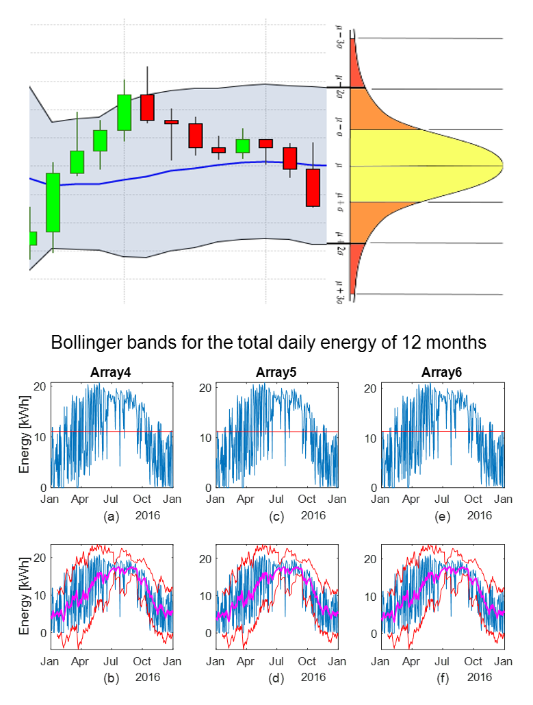
4.4. Twelve-Months Analysis (January–December 2016)

This dataset contains 366 samples per array and each sample is the sum of 144 energy measurements per day. Figure 9 and Figure 10 and

Table 4. Mean energy and spread with respect to the global mean for the twelve-months analysis.

Array	1	2	3	4	5	6
Mean (kWh)	11.59	11.01	11.28	11.10	11.17	11.33
Global mean	11.21
Spread %	1.20	−1.72	0.66	−0.94	−0.35	1.15

contain information such as those of Figure 3 and Figure 4 and Table 1, but they refer to a longer time, i.e., January–December 2016.

By comparing the energy produced by the arrays (first row of Figure 9 and Figure 10), it turns out that the time-series and the mean values are very similar. This is confirmed by the data in Table 4. In fact, the spread never exceeds 3%. Focusing attention on the BB, it turns out that the choice of 1.5σ for upper and lower bands allows to constrain the produced energy diagram within the BB, except for the July peak and some punctual overruns. Furthermore, it turns out that the width increases after the summer, i.e., the volatility increases, because the weather becomes unstable. Combined information of time-series within the BB and spreads less than the alert threshold returns feedback that no criticality is present. It is important to note that in the October–December period, the diagram of the produced energy frequently touches the lower band, which acts as “support”—that is, a known behavior in the financial field when a price is decreasing [31].

Table 5. Spread of each array in each period.

${\mathit{S}}_{\mathit{k}}\left(\mathit{\%}\right)$	1	2	3	4	5	6
3 months	0.76	−1.73	0.76	−0.40	−0.28	0.91
6 months	1.54	−1.75	0.86	−1.16	−0.35	0.86
9 months	1.46	−1.65	0.81	−1.18	−0.25	0.81
12 months	1.20	−1.72	0.66	−0.94	−0.35	1.15

groups the spreads of each array in the four analyzed periods. It turns out that arrays #1, #3, and #6 always have positive spreads, and vice versa for the arrays #2, #4 and #5. Therefore, there are three arrays (#1, #3, and #6) that produce more energy than the other three arrays (#2, #4, and #5) in any analyzed period. Moreover, array #1 is the best one in any period, apart from the first period (0.76). It probably has the best sun exposure. Instead, array #2 is the worst one in any period; even if it never exceeds the 3% threshold, it requires specific attention to understand if the low values are due to an external cause (e.g., partial shading for an obstacle) or to premature aging. Array #5 has values closer to zero than other arrays in any period; therefore, its behavior is representative of the average behavior of the PV system. Arrays #3, #4, and #6 have values around 1% almost always.

4.5. Comparison among Simple, Linear and Exponential MA

The BB of the previous analyses were based on EMA, whereas the standard application of the BB considers SMA or LMA. John Bollinger advices to always use 20 periods for MA to avoid false signals. For financial purposes, the upper and lower bands are defined as $UB/LB=AVG\pm 2\sigma$, and the width is 4σ. This choice is too large to analyze the energy data of a PV plant, because its volatility is limited during the whole year. In fact, whatever the environmental conditions in a whole year, the energy time series of each arrays always has the typical quasi-Gaussian waveform represented by the magenta curves in Figure 9 and Figure 10. As a result, the yearly variability of the atmospheric phenomena on the same PV plant, installed in the same place, is limited. However, too large a space between the upper and lower bands is as ineffective as too small a space. After many applications on different energy datasets of different PV plants, the optimal choice returns a width of 3σ, i.e., $UB/LB=AVG\pm 1.5\sigma$. A comparison among the BB based on SMA, LMA, and EMA is reported in Figure 11. The three cases are based on the same parameters: 20 periods for the MA and $F=1.5$. The black arrows indicate the samples out of the BB: 14 samples for SMA, 9 for LMA, and 6 for EMA. Therefore, the width based on EMA is the best fitting.

5. Conclusions

The proposed statistical approach to supervise the performance of multi-array and small- to medium-rated power (3–50 kWp) PV plants is useful when meteorological data are not available. The procedure is cumulative because new energy samples are added to the previous ones before starting the new statistical analysis. The case study is a real operating PV system and the cumulative dataset is based on three, six, nine, and twelve months. The paper introduces two important modifications to the standard BB method. The former one is to use EMA₂₀ instead of SMA₂₀ or LMA₂₀. The latter one is to set F = 1.5 instead of F = 2. The results of the case study with these new settings allow several considerations. The BB method can follow the variability of the energy performance of a PV plant due to the variability of the environmental conditions. In fact, the narrow channel of the BB during the summer depends on the low variability of the environmental conditions in that season, and vice versa in the other seasons. However, BB are calculated for each single array, without any correlation with the other arrays; therefore, even if BB method can detect a strong failure in a single array, it cannot detect a low-intensity anomaly. This implies that the BB method is able to detect even a low-intensity anomaly only if used in combination with at least one other index, which allows to compare the energy performance of the arrays. This paper has proposed use of the relative percentual spread to support the BB method, but future work will be focused in exploring the effectiveness of other statistical tools.

References

1. Xiao, W.; Ozog, N.; Dundorf, W.G. Topology study of photovoltaic interface for maximum power point tracking. IEEE Trans. Ind. Electron. 2007, 54, 1696–1704. [Google Scholar] [CrossRef]
2. Mutoh, N.; Inoue, T. A control method to charge series- connected ultraelectric double- layer capacitors suitable for photovoltaic generation systems combining MPPT control method. IEEE Trans. Ind. Electron. 2007, 54, 374–383. [Google Scholar] [CrossRef] [Green Version]
3. Grimaccia, F.; Leva, S.; Mussetta, M.; Ogliari, E. ANN Sizing Procedure for the Day-Ahead Output Power Forecast of a PV Plant. Appl. Sci. 2017, 7, 622. [Google Scholar] [CrossRef] [Green Version]
4. Acciani, G.; Chiarantoni, E.; Fornarelli, G.; Vergura, S. A feature extraction unsupervised neural network for an environmental data set. Neural Netw. 2003, 16, 427–436. [Google Scholar] [CrossRef]
5. Vergura, S.; Pavan, A.M. On the photovoltaic explicit empirical model: Operations along the current-voltage curve. In Proceedings of the 2015 International Conference on Clean Electrical Power (ICCEP), Taormina, Italy, 16–18 June 2015. [Google Scholar]
6. Pavan, A.M.; Vergura, S.; Mellit, A.; Lughi, V. Explicit empirical model for photovoltaic devices. Experimental validation. Sol. Energy 2017, 155, 647–653. [Google Scholar] [CrossRef] [Green Version]
7. Guerriero, P.; di Napoli, F.; Vallone, G.; D’Alessandro, V.; Daliento, S. Monitoring and diagnostics of PV plants by a wireless self-powered sensor for individual panels. IEEE J. Photovolt. 2015, 6, 286–294. [Google Scholar] [CrossRef]
8. Takashima, T.; Yamaguchi, J.; Otani, K.; Kato, K.; Ishida, M. Experimental Studies of Failure Detection Methods in PV module strings. In Proceedings of the 2006 IEEE 4th World Conference on Photovoltaic Energy Conversion, Waikoloa, HI, USA, 7–12 May 2006; Volume 2, pp. 2227–2230. [Google Scholar]
9. Breitenstein, O.; Rakotoniaina, J.P.; Al Rifai, M.H. Quantitative evaluation of shunts in solar cells by lock-in thermography. Prog. Photovolt. Res. Appl. 2003, 11, 515–526. [Google Scholar] [CrossRef]
10. Vergura, S.; Marino, F.; Carpentieri, M. Carpentieri, Processing Infrared Image of PV Modules for Defects Classification. In Proceedings of the International Conference on Renewable Energy Research and Applications (ICRERA 2015), Palermo, Italy, 22–25 November 2015; ISBN 978-1-4799-9981-1. [Google Scholar]
11. Grimaccia, F.; Leva, S.; Dolara, A.; Aghaei, M. Survey on PV Modules’ Common Faults after an O&M Flight Extensive Campaign over Different Plants in Italy. IEEE J. Photovolt. 2017, 7, 810–816. [Google Scholar]
12. Johnston, S.; Guthrey, H.; Yan, F.; Zaunbrecher, K.; Al-Jassim, M.; Rakotoniaina, P.; Kaes, M. Correlating multicrystalline silicon defect types using photoluminescence, defect-band emission, and lock-in thermography imaging techniques. IEEE J. Photovolt. 2014, 4, 348–354. [Google Scholar] [CrossRef]
13. Peloso, M.P.; Meng, L.; Bhatia, C.S. Combined thermography and luminescence imaging to characterize the spatial performance of multicrystalline Si wafer solar cells. IEEE J. Photovolt. 2015, 5, 102–111. [Google Scholar] [CrossRef]
14. Vergura, S.; Marino, F. Quantitative and Computer Aided Thermography-based Diagnostics for PV Devices: Part I—Framework. IEEE J. Photovolt. 2017, 7, 822–827. [Google Scholar] [CrossRef]
15. Vergura, S.; Colaprico, M.; de Ruvo, M.F.; Marino, F. A Quantitative and Computer Aided Thermography-based Diagnostics for PV Devices: Part II—Platform and Results. IEEE J. Photovolt. 2017, 7, 237–243. [Google Scholar] [CrossRef]
16. Mekki, H.; Mellit, A.; Salhi, H. Artificial neural network-based modelling and fault detection of partial shaded photovoltaic modules. Simul. Model. Pract. Theory 2016, 67, 1–13. [Google Scholar] [CrossRef]
17. Harrou, F.; Sun, Y.; Kara, K.; Chouder, A.; Silvestre, S.; Garoudja, E. Statistical fault detection in photovoltaic systems. Sol. Energy 2017, 150, 485–499. [Google Scholar]
18. Vergura, S. Hypothesis Tests-Based Analysis for Anomaly Detection in Photovoltaic Systems in the Absence of Environmental Parameters. Energies 2018, 11, 485. [Google Scholar] [CrossRef] [Green Version]
19. Cristaldi, L.; Faifer, M.; Leone, G.; Vergura, S. Reference Strings for Statistical Monitoring of the Energy Performance of Photovoltaic Fields. In Proceedings of the IEEE-ICCEP 2015 International Conference on Clean Electrical Power, Taormina, Italy, 16–18 June 2015. [Google Scholar]
20. Ventura, C.; Tina, G.M. Development of models for online diagnostic and energy assessment analysis of PV power plants: The study case of 1 MW Sicilian PV plant. Energy Procedia 2015, 83, 248–257. [Google Scholar] [CrossRef] [Green Version]
21. Silvestre, S.; Kichou, S.; Chouder, A.; Nofuentes, G.; Karatepe, E. Analysis of current and voltage indicators in grid connected PV (photovoltaic) systems working in faulty and partial shading conditions. Energy 2015, 86, 42–50. [Google Scholar] [CrossRef]
22. Vergura, S. Scalable Model of PV Cell in Variable Environment Condition based on the Manufacturer Datasheet for Circuit Simulation. In Proceedings of the 2015 IEEE 15th International Conference on Environment and Electrical Engineering (EEEIC), Roma, Italy, 10–13 June 2015. [Google Scholar]
23. Chao, K.H.; Ho, S.H.; Wang, M.H. Modeling and fault diagnosis of a photovoltaic system. Electr. Power Syst. Res. 2008, 78, 97–105. [Google Scholar] [CrossRef]
24. Hamdaoui, M.; Rabhi, A.; Hajjaji, A.; Rahmoum, M.; Azizi, M. Monitoring and control of the performances for photovoltaic systems. In Proceedings of the International Renewable Energy Congress, Sousse, Tunisia, 5–7 November 2009. [Google Scholar]
25. Kim, I.-S. On-line fault detection algorithm of a photovoltaic system using wavelet transform. Sol. Energy 2016, 226, 137–145. [Google Scholar] [CrossRef]
26. Rabhia, A.; El Hajjajia, A.; Tinab, M.H.; Alia, G.M. Real time fault detection in photovoltaic systems. Energy Procedia 2017, 11, 914–923. [Google Scholar]
27. Plato, R.; Martel, J.; Woodruff, N.; Chau, T.Y. Online fault detection in PV systems. IEEE Trans. Sustain. Energy 2015, 6, 1200–1207. [Google Scholar] [CrossRef]
28. Ando, B.; Bagalio, A.; Pistorio, A. Sentinella: Smart monitoring of photovoltaic systems at panel level. IEEE Trans. Instrum. Meas. 2015, 64, 2188–2199. [Google Scholar] [CrossRef]
29. Harrou, F.; Sun, Y.; Taghezouit, B.; Saidi, A.; Hamlati, M.E. Reliable fault detection and diagnosis of photovoltaic systems based on statistical monitoring approaches. Renew. Energy 2018, 116, 22–37. [Google Scholar] [CrossRef] [Green Version]