Constrained Generation Bids in Local Electricity Markets: A Semantic Approach

Abstract

The worldwide investment in renewable energy sources is leading to the formation of local energy communities in which users can trade electric energy locally. Regulations and the required enablers for effective transactions in this new context are currently being designed. Hence, the development of software tools to support local transactions is still at an early stage and faces the challenge of constant updates to the data models and business rules. The present paper proposes a novel approach for the development of software tools to solve auction-based local electricity markets, considering the special needs of local energy communities. The proposed approach considers constrained bids that can increase the effectiveness of distributed generation use. The proposed method takes advantage of semantic web technologies, in order to provide models with the required dynamism to overcome the issues related to the constant changes in data and business models. Using such techniques allows the system to be agnostic to the data model and business rules. The proposed solution includes the proposed constraints, application ontology, and semantic rule templates. The paper includes a case study based on real data that illustrates the advantages of using the proposed solution in a community with 27 consumers.

1. Introduction

On 5 June 2019, the European Parliament launched the Directive (EU) 2019/9442 “on common rules for the internal market for electricity and amending Directive 2012/27/EU” [1]. This new directive introduces significant changes in the business models and electricity markets, intending to provide a real choice to all of the Union’s final consumers, creating new business opportunities, offering competitive prices, showing signs of effective investments and ensuring higher service standards, as well as contributing to the security of supply and sustainability [2]. The common goal of decarbonizing the energy system creates new opportunities and poses new challenges to market participants [3]. Technological developments allow new forms of consumer participation and cross-border cooperation [4]. In this way, this new directive adjusts the Union’s market rules to a new market reality. In addition to responding to new challenges, this Directive also aims to find solutions to overcome the remaining obstacles to the effective and efficient implementation of the internal electricity market [5]. Thus, this directive incentivizes the development of new business models, which are significantly different from those that are currently possible.

Across the globe, financial and environmental concerns are leading to a reduction in carbon emissions and to the improvement of system security and affordability of power and energy systems by promoting the integration of distributed generation (DG) into the power system [6]. To this end, governments are encouraging the use of renewable energy sources (RES) [7] along with information and communication technology (ICT) [8] devices to form so-called energy communities where end users can trade energy [9,10]. These communities are already a reality in some pilot microgrid and smart grid (SG) projects [9,10,11,12,13]. SGs take advantage of ICT to enable the bi-directional flow of energy while providing the fully automated monitoring, control, and protection of the grid [14], fulfilling the supply of sustainable, secure, and economical energy and considering the participation of active end users.

End consumers, who can both generate and consume energy, are called prosumers. Prosumers can curtail, trade, store, or send their surplus energy to the power grid. These players are mainly motivated by financial incentives, environmental concerns, and low levels of trust in energy suppliers [15,16]. Local electricity markets enable small-scale players to trade within their communities, promoting the local grid balance, reducing the cost of electricity bills, incentivizing the investment in RES, and supporting a self-sustained SG community [17,18]. Several works present solutions to solve local electricity markets for various purposes, such as peer-to-peer [10,15,16], blockchain [11,19], bidding [20,21,22,23], bilateral negotiation [24,25] and constrained markets [26], among others.

The application of constrained bids in competitive markets has been explored in the literature, mostly through theoretical analyses of the impact of this type of bid on the market equilibrium and players’ results [27,28,29]. However, the literature lacks works that address the application of constrained bids in local electricity market environments. Different types of restrictions may be applied in this context, namely constraints intrinsic to the distribution network, as well as constraints on the users’ aggregation contracts [30,31]. Additionally, when considering auction-based transactions, players should also be able to determine constraints making the local market more competitive and attractive to its participants. In fact, not only are adequate models to support players’ actions in local electricity markets lacking, but the development of software to solve local electricity market transactions is also at an early stage. Accommodating the novel and constantly changing business rules may become a burden due to their volatile nature. Any update to the system requires it to be reprogrammed and recompiled. Ideally, the system should be abstracted from the data model and the business rules and receive them as inputs. In this way, the system would only need to be reprogrammed when the business model changes significantly.

In the present paper, a novel approach is proposed to develop tools to solve auction-based local electricity market transactions, considering constrained bids. The proposed approach overcomes programming issues, making the system more flexible and adaptable to the evolution of local market rules. To this end, we take advantage of ontologies and semantic web technologies to keep the system agnostic to the data model and business rules. The use of ontologies and semantic web technologies provides the means to develop systems decoupled from the data models and business rules. These techniques enable the development of systems with a higher flexibility, avoiding the need for reprogramming whenever the data models or business rules need to be updated. Additionally, when using these technologies, systems are able to perform reasoning upon data since semantic models provide context and information about data. The proposed constrained bids are developed specifically for local market transactions, in order to enable players to improve the potential outcomes from market participation by providing them with the means to incorporate strategic information into their—otherwise straightforward—bids. In this way, the players are able to specify the conditions of their offers regarding distributed generation, which can sometimes be difficult to model, as the modeled constraints can be conflicting in the search for optimal solutions. The proposed model offers a different product for local markets that considers constraints that will ease players’ participation in local markets. Therefore, it allows for the incentivization of increased consumer participation, by offering options that allow local trading to be performed according to players’ interests, objectives, strategic needs and preferences. Each player is able to select the constraints that are more relevant and easier to use, according to their reality and preferences.

The following section provides the background on auction-based electricity market types, local market bid constraints, and the advantages of using ontologies and semantic web technologies instead of coding data models and business rules. Section 3 presents the proposed solution to solve constrained transactions in local electricity markets while keeping the system flexible to test different alternatives. It will detail the defined constraints, the ontology designed and used to describe the data and business models, and the semantic rules developed for each specified constraint. The case study presented in Section 4 illustrates the operation of the developed software tool, focusing on the use of the semantic rules. The conclusions about the developed work are presented in Section 5.

2. Background

Local electricity markets are the future in the decentralization of power and energy systems, focusing on consumers, energy efficiency, and distributed micro generation [1,2,4,5]. In recent years, a growing interest in the study and development of local electricity markets has emerged, namely in peer-to-peer [10,15,16], blockchains [11,19], transactive energy [9,21,32], and demand response (DR) [33,34], among others. This section provides the background of the different domains brought together to compose the proposed solution. These domains are auction-based local electricity market types, local market bid constraints, and ontologies and semantic web technologies. Section 2.1 gives an overview of the auction-based local market types proposed in the literature, while Section 2.2 presents the ontologies and semantic web technologies, explaining why their use is considered in the proposed approach.

2.1. Auction-Based Local Electricity Market Types

Auction-based local electricity markets are addressed in the literature [20,21,22,23]. The most common trading designs are the double auction [20,21] (symmetric), and the single-sided auction [22,23] (asymmetric). In symmetric market pools [35,36], both buyers and sellers compete by submitting their bids. In electricity markets, a bid is a pair made up of the amount of energy to trade and the price per unit. Bids from buyers are ordered by price in descending order, while seller bids are ordered ascendingly. These bids form the demand and supply step curves. The point where both curves intersect (Figure 1a) determines the amount of energy to trade, while the market price is set by the last seller to sell. Buyer bids offering prices higher than the market price and seller bids offering prices lower than the market price trade in the market pool. In the end, each buyer must pay the market price per each accepted supply unit.

On the other hand, in asymmetric market pools, only sellers submit energy/price bids, while buyers only submit their demand. The seller bids are ordered by price ascendingly. The sum of the buyers’ required energy sets the total demand. The seller bids are accepted until the total demand is satisfied. The last seller to trade sets the market price that buyers must pay per each energy unit traded (Figure 1b).

The most common types of local market constraints found in the literature are related to network limitations, such as the capacity of the distribution lines, congestion management, voltage deviations and thermal limits, among others [26,30,31]. The work presented in the present paper goes forward in exploring the bid constraints that local market players can submit, in order to have their preferences respected, so buyers can easily say how much and when they want to buy, and sellers can easily say how much and when they want to sell. In this way, the players are able to specify the conditions of their offers regarding distributed generation. As a result, the authors decided to design, develop, and propose constraints that make sense, are interesting, and attractive for local market participants so they participate more, and with a greater amount of energy. Section 3.1 details these constraints.

2.2. Ontologies and Semantic Web Technologies

In computer science, ontologies conceptualize meaningful descriptions of the domains’ abstract and rational models, describing their concepts, properties, and the relations between them. Their formal and explicit representation enables both humans and machines to comprehend them and reason upon them [37,38]. They allow knowledge sharing, reuse, and common understanding across heterogeneous entities. Moreover, they provide computational inference, through inference engines, on conceptual models and stored data, enabling the automatic generation of new knowledge [39].

“The W3C Web Ontology Language (OWL) is a Semantic Web language designed to represent rich and complex knowledge about things, groups of things, and relations between things” [40]. In other words, OWL is designed to represent ontologies on the world wide web (WWW). It eases the machine readability and the interpretation of information content while providing a means for knowledge inference. OWL 2 [41] is the latest version published and it is usually written in Resource Description Framework (RDF). RDF [42] is a language designed to represent data about web resources. It uses Uniform Resource Identifiers (URI) to describe resources and relationships between them, setting triples in the form of “<subject> <predicate> <object>”. This structure creates directed, labeled graphs providing a consistent and standard way to describe and query resources on the web. The graph view is the easiest mental model for easy-to-understand explanations. The RDF allows information to be exchanged between applications without losing its meaning. Its vocabulary is defined by RDF Schema (https://www.w3.org/TR/rdf-schema/), which describes the RDF’s abstract syntax and basic concepts, its formal semantics, and serialization syntaxes. There are different serialization formats available to write RDF graphs, such as RDF/Extensible Markup Language (XML, https://www.w3.org/TR/rdf-syntax-grammar/), JavaScript Object Notation for Linked Data (JSON-LD) (https://www.w3.org/TR/json-ld11/) and Turtle (https://www.w3.org/TR/turtle/), among others.

Triple stores, or RDF stores, are databases designed for the storage and retrieval of data triples through semantic queries [43]. Semantic queries process structured data, such as triples, named graphs, and linked data. The WWW Consortium (W3C) recommends the SPARQL Protocol and RDF Query Language [44] (SPARQL) as an RDF query language. SPARQL 1.1 is considered one of the key technologies of the semantic web as it provides protocols to query and manipulate RDF graphs. SPARQL query results are retrieved in one of the following well-known formats: (i) Extensible Markup Language (XML); (ii) JavaScript Object Notation (JSON); (iii) Comma Separated Values (CSV); (iv) Tab-Separated Values (TSV).

In summary, semantic web technologies provide a common framework to: (1) define data models and represent data through them, understandable by both humans and machines; (2) ease interoperability between software tools by sharing both the data and the models; (3) store, query, and manipulate these structured data and models. Other advantages of using the semantic web framework are the possibility of keeping the data model decoupled from the software and the use of SPARQL to implement the business rules, as exemplified in [45]. In this way, developed systems can be more flexible and configurable, avoiding the need to reprogram them when the data model or a rule is updated as much as possible. The following section will demonstrate how this is achieved.

3. Proposed Semantic-Based Constrained Bid Model

The proposed semantic-based constrained bid model for local electricity markets aims to be used to manage auction-based local electricity markets and for studying and testing them in the scope of simulation systems. The model is written as a code library so it can be reused by different systems and tools, including agent-based systems, desktop applications, and web services. Keeping in mind the need to develop a flexible and configurable system able to address different alternatives to solve auction-based transactions, considering constrained bids in local electricity markets, the following requirements where defined:

• the system must take advantage of semantic web technologies;
• the semantic model(s) must describe all the required knowledge;
• the system must be agnostic to the semantic model(s) used;
• the connection to the triple store must be configurable;
• SPARQL must be used to query/update the knowledge base (KB);
• the system must be agnostic to the bid’s constraints;
• the bids’ constraints must be written in SPARQL;
• the bids’ constraints must be configurable.

In the present work, the proposed solution is applied and driven to a smart grid aggregator aimed at local communities with around 100 players. For this community size, the proposed methodology takes around five minutes to run a complete market session. The aggregator is modelled as a software agent of an agent-based smart grid simulation platform developed with the Java Agent Development framework (JADE) [46]. Therefore, this library was developed in Java [47] programming language, and uses Apache Jena Fuseki [48] as the triple store. 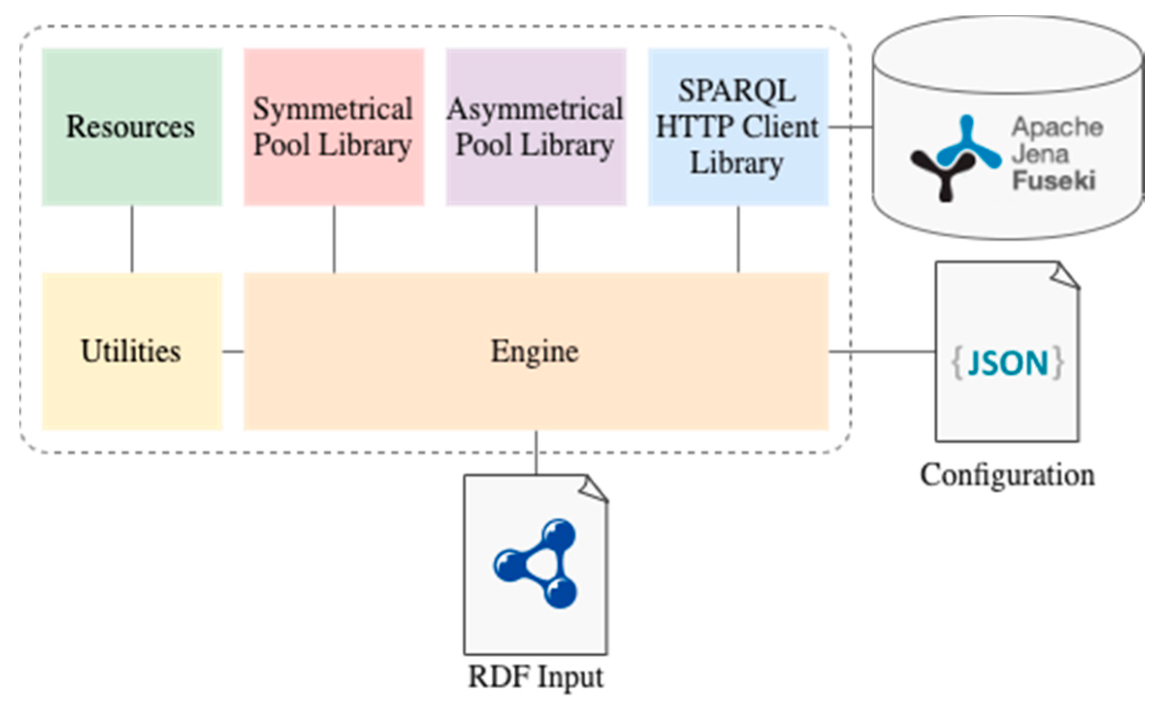Figure 2 illustrates the architecture of the library designed and developed.

The local market library receives, as an input, an RDF KB file, as well as a configuration JSON file. The RDF KB file has the input data necessary to run the local auction-based market algorithm, detailing the type of market pool to run (symmetric, by default, or asymmetric), the session and respective periods, and the players’ bids and constraints. The configuration JSON file detains information about the KB file path and its RDF language (such as Turtle, RDF/XML, JSON-LD, etc.), Fuseki server configuration, and the local market constraint templates for each possible bid constraint. The configuration file makes the use of remote KB files, as well as the different SPARQL triple stores available, and also the addition, updating, or removal of constraint templates much easier, without the need to reprogram the system.

The library itself is composed of three packages, namely the Engine, the Resources, and Utilities, and imports three libraries developed during the present work: the Symmetrical Pool Library, the Asymmetrical Pool Library, and the SPARQL HTTP Client Library. The first two libraries are to execute each of the auction-based market pool algorithms: the double auction and the single-sided auction, respectively. The third library provides a SPARQL over an HTTP (SOH) client to communicate with any triple store compliant with SPARQL 1.1. The Utilities package provides general useful methods, as well as access to the Resources files necessary to manage data from the triple store. These resource files include configuration JSON schemas to validate both the input configuration file and the results output, as well as SPARQL queries and updates to manage the KB data during the system’s execution.

The Engine is the core package that, using all the abovementioned features, makes the library run smoothly. To keep the system agnostic to the data model, the Engine uses JSON objects instead of Java classes. The resource SPARQL query files used to obtain the data from the KB return JSON strings that respect predetermined JSON schemas used by the Engine. Thus, the ontology may change without the need to reprogram the system, as long as it is possible to get the same JSON strings from the accordingly updated SPARQL queries.

The following subsections detail the defined bid constraints (Section 3.1), the application ontology (Section 3.2), and each constraint’s SPARQL template (Section 3.3).

3.1. Bid Constraints for Auction-Based Local Electricity Market

In order to overcome the gap in the literature regarding bid constraints for auction-based local electricity markets, this work proposes new constrained bid models for this type of exchange. The authors consider different types of constraints, namely session and period constraints. Additionally, some constraints are directed to buyers and others to suppliers. The proposed constraints for each session (typically composed of a set of four periods) are Minimum Income, Maximum Cost, Minimum Matched Energy, and Maximum Matched Energy. For each period, the proposed constraints are Minimum Matched Energy, and Maximum Matched Energy. These proposed bid constraints were designed for the symmetric pool. However, if desired, some may be applied to the asymmetric market, namely the ones related to the suppliers.

The motivation for the definition and use of such constraints include the following aspects:

-

allowing a single, small-size player to bound its participation, and probably increase the number of players actively participating as they can be surer that bidding actions will not be disadvantageous for them;

-

as consequence, this allows an increase in the competitiveness of the local market as more players are participating;

-

some players can be motivated by profit, while other can be motivated, for example, by the amount of negotiated energy, so adequate modeling of both types of motivations should be accommodated;

-

the risk or unpredictability of a bid to be accepted is sometimes not easy to handle by a local player of a small size. With the implemented constraints, the player can make more risky bids in terms of price in specific periods, at the same time ensuring that a certain amount of remuneration must be respected in the session;

-

some players may want to always have an accepted bid, while other players may disregard the single-period results and bind their objectives regarding the session;

-

the possibility of different players selecting different constraints they want to use makes it possible to keep simple models for each player;

-

in this way, it is important to find a way in which some players can choose certain constraints, then disregard the remaining constraints, while other players can choose other constraints that are more relevant for them.

It should be highlighted that adding these constraints to the local market model make it more complex, and it is hard for players to understand how the price was formed. However, the way in which the increased participation of players in the local market can be obtained is an advantage, putting the complexity burden on the retailer side.

The Minimum Income for a session is a constraint that sets a minimum acceptable value for the player’s total income, as presented in Equation (1). Suppliers submitting this constraint do not want to participate in the market session unless the total income A is reached.

$${\displaystyle \sum }_{t=1}^T\left[E_{\left(t\right)}\times Price.M_{\left(t\right)}\right]\ge A$$

(1)

where:

• $E_{\left(t\right)}$—energy transacted in period $t$;
• $Price.M_{\left(t\right)}$—market price of period $t$;
• $A$—the minimum income set by the player;
• $T$—the session’s total number of periods.

Additionally, the Minimum Income also sets a lower bound of the session’s average price per kWh and must be higher or equal to the value B submitted in Equation (2).

$$\frac{{\sum }_{t=1}^T\left[E_{\left(t\right)}\times Price.M_{\left(t\right)}\right]}{{\sum }_{t=1}^T\left[E_{\left(t\right)}\right]}\ge B$$

(2)

where:

• $E_{\left(t\right)}$—energy transacted in period $t$;
• $Price.M_{\left(t\right)}$—market price of period $t$;
• $B$—the minimum average price per kWh set by the player;
• $T$—the session’s total number of periods.

The Maximum Cost session constraint is the opposite of the Minimum Income. It sets a maximum acceptable value for the player to pay at the end of the session. Buyers submitting this restriction do not want to participate in the session if their costs are higher than the total cost value C set in this rule, as presented in Equation (3).

$${\displaystyle \sum }_{t=1}^T\left[E_{\left(t\right)}\times Price.M_{\left(t\right)}\right]\le C$$

(3)

where:

• $E_{\left(t\right)}$—energy transacted in period $t$;
• $Price.M_{\left(t\right)}$—market price of period $t$;
• $C$—the maximum cost set by the player;
• $T$—the session’s total number of periods.

Likewise, the Maximum Cost additionally sets a maximum price to pay per kWh. Buyers submitting this restriction do not want to participate in the session if the average price paid per kWh is higher than value D, as presented in Equation (4).

$$\frac{{\sum }_{t=1}^T\left[E_{\left(t\right)}\times Price.M_{\left(t\right)}\right]}{{\sum }_{t=1}^T\left[E_{\left(t\right)}\right]}\le D$$

(4)

where:

• $E_{\left(t\right)}$—energy transacted in period $t$;
• $Price.M_{\left(t\right)}$—market price of period $t$;
• $D$—the maximum average price per kWh set by the player;
• $T$—the session’s total number of periods.

The Minimum Matched Energy session constraint sets a minimum energy amount to trade in the market session. Players submitting this constraint do not want to participate in the market session unless their total transacted energy is higher or equal to the minimum amount F set, as presented in Equation (5).

$${\displaystyle \sum }_{t=1}^T{E}_{\left(t\right)}\ge F$$

(5)

where:

• $E_{\left(t\right)}$—energy transacted in period $t$;
• $F$—the minimum amount of energy to trade set by the player;
• $T$—the session’s total number of periods.

The Maximum Matched Energy session constraint, in opposition to the above Minimum Matched Energy, determines a maximum energy amount to trade in the market session. Players setting this restriction only want to participate in the market session if their total transacted energy is lower than or equal to the maximum amount submitted G, as presented in Equation (6).

$${\displaystyle \sum }_{t=1}^T{E}_{\left(t\right)}\le G$$

(6)

where:

• $E_{\left(t\right)}$—energy transacted in period $t$;
• $G$—the maximum amount of energy to trade set by the player;
• $T$—the session’s total number of periods.

Regarding period constraints, the Minimum Matched Energy period constraint is similar to the Minimum Matched Energy session constraint but applied in a specific period. Players applying this constraint do not want to participate in the period’s pool unless their traded energy is higher or equal to the predetermined amount H, as presented in Equation (7).

$$Bi{n}_{\left(t\right)}\times E_{\left(t\right)}\ge H, \forall t\in \left[1:T\right]$$

(7)

where:

• $Bi{n}_{\left(t\right)}$—Decision variable regarding the participation in period t;
• $E_{\left(t\right)}$—energy transacted in period $p$;
• $H$—the minimum amount of energy to trade set by the player;
• $T$—the session’s total number of periods.

The Maximum Matched Energy period constraint is the opposite of the Minimum Matched Energy period constraint as it sets a maximum trade amount for the given period. Players using this restriction only want to participate in the period’s pool if the traded energy is lower than or equal to the amount defined I, as presented in Equation (8).

$$Bi{n}_{\left(t\right)}\times E_{\left(t\right)}\le I, \forall t\in \left[1:T\right]$$

(8)

where:

• $Bi{n}_{\left(t\right)}$—Decision variable regarding the participation in period t;
• $E_{\left(t\right)}$—energy transacted in period $t$;
• $X$—the maximum amount of energy to trade set by the player;
• $T$—the session’s total number of periods.

These restrictions are a good starting point to test and study the impact of constrained bids in local electricity markets. It should be noted that the order in which these constraints are triggered determines the market’s outcomes. However, the constraints’ priorities must be previously defined by proper legislation and also exposed to the players in their contracts to make the market fair and clear to every participant, so they can take full advantage of participating. The developed system enables the configuration of each constraint’s priority within the semantic model, avoiding the need to reprogram the system every time a user wants to try a different configuration. The constraints’ priorities do not change during the system’s execution.

3.2. Application Ontology

The application ontology represents all of the system’s required knowledge, from the data model to the business rules. Since the system must be agnostic to the semantic model used, an application ontology has been specifically developed for test and proof purposes. However, the developed library enables the user to use another ontology, as long as the resource files, configuration files, and SPARQL rules are updated accordingly. This section briefly presents the Local Market Ontology (LMO), introducing the required concepts for the system to work properly. Not being the main result of this work, the development process of LMO will not be described in great detail. The LMO application ontology has been developed using the 101 development methodology [49]. Its domain and scope are the local auction-based electricity markets with constrained bids. LMO is publicly available (http://www.gecad.isep.ipp.pt/mdpi/energies/845690/files/onto/local-market.ttl).

Reusing existing ontologies is one of the first steps in the development process as it is good practice [49]. Publicly available ontologies facilitate interoperability between heterogeneous systems, as well as knowledge reuse and extension. Thus, the Electricity Market Ontology [50] (EMO) was reused and extended to include the necessary concepts and relations for local market execution. It is publicly available a modular ontology (http://www.mascem.gecad.isep.ipp.pt/ontologies/), developed to provide semantic interoperability with the Multi-Agent Simulator of Competitive Electricity Markets (MASCEM) [51]. Its modular design eases the extension and reuse of the necessary concepts and relations. The LMO application ontology imports and extends the Call for Proposal (CfP) ontology and the Electricity Market Results (EMR) ontology [52], which already import EMO’s high-level module.

Table 1. Local Market Ontology (LMO)’s classes, properties, and facets.

Class	Properties	Facets
Constraint	priority	1 unsignedInt
HourAhead		emo:MarketType
HourAheadSession		emo:Session
LocalMarket		emo:Market
MaximumCost	hasTotalCost pricePerkWh	Constraint 1 emo:Price 1 emo:Price
MaximumMatchedEnergy	emo:hasPower emo:placedInPeriod	Constraint 1 emo:Power emo:Period
MinimumIncome	hasTotalIncome pricePerkWh	Constraint 1 emo:Price 1 emo:Price
MinimumMatchedEnergy	emo:hasPower emo:placedInPeriod	Constraint 1 emo:Power emo:Period
cfp:Proposal	instant emr:fromPlayer	1 unsignedLong 1 emo:Player
emr:BidResult	wasTraded	1 boolean
emo:Player	setPeriodConstraint setPeriodsConstraint setSessionConstraint totalBoughtEnergy totalCost totalIncome totalSoldEnergy totalTransactedEnegy	Constraint Constraint Constraint 1 emr:TradedPower 1 emo:Price 1 emo:Price 1 emr:TradedPower 1 emr:TradedPower

presents LMO’s classes, as well as their properties and facets. The object properties, properties that relate concepts with each other, are written in blue. The datatype properties, properties that relate concepts with their values, are in green.

Constraint is the top-level class for the bid constraints. Any bid constraints defined for the local auction-based market must be subclasses of this class. This class is defined by one unsigned integer priority datatype property, which sets the order in which the bid constraints must be checked.

The HourAhead, HourAheadSession, and LocalMarket classes are subclasses of the EMO’s classes emo:MarketType, emo:Session, and emo:Market, respectively. Although these classes do not declare any new properties, they inherit their super-classes’ properties (available at [50]).

The MaximumCost is a subclass of Constraint. It describes the constraint defined in Equations (3) and (4). As well as the inherited priority datatype property, it is also defined by the hasTotalCost and the pricePerkWh object properties. The hasTotalCost object property defines the maximum cost that the player will pay, using one instance of EMO’s emo:Price class. Similarly, the pricePerkWh object property defines the maximum accepted price per kWh to be paid.

The MaximumMatchedEnergy is also a subclass of Constraint, describing the constraints defined in Equations (6) and (8). This constraint was designed to be used in both equations since the parameter is the same. By extending Constraint, it inherits the priority datatype property. It is also defined by the EMO’s emo:hasPower object property that relates to an instance of EMO’s emo:Power class, determining the maximum amount of matched energy. Finally, when using this class as a period constraint, the emo:placedInPeriod object property must be used to determine the period in which this rule applies. This property relates to EMO’s emo:Period classes, enabling us to assign the same value to different periods.

MinimumIncome is another subclass of Constraint. It describes the constraint of Equations (1) and (2). Its definition is similar to the MaximumCost class, being the difference in the use of the hasTotalIncome object property instead of hasTotalCost.

The MinimumMatchedEnergy is, again, a subclass of Constraint and describes the constraints defined in Equations (5) and (7). Similarly, this class was designed to be used in both Session and Period equations. It is defined exactly as the MaximumMatchedEnergy class. However, the name of the class informs the system which SPARQL rule applies.

The CfP’s cfp:Proposal was extended to add two important details for the aggregator’s KB. One is the instant the aggregator receives the player’s proposal as an unsigned long timestamp in milliseconds. The second is the information about the player presenting the proposal, using the EMR’s emr:fromPlayer object property.

The EMR’s emr:BidResult class was also extended with a new datatype property, wasTraded. It sets whether a player’s bid was traded or not, after a pool execution.

The EMO’s emo:Player class was redefined by adding eight new object properties. The setPeriodConstraint, setPeriodsConstraint, and setSessionConstraint object properties relate to the Constraint class. They enable the definition of period and session constraints for a given player. The setPeriodsConstraint object property is used with constraints for multiple periods, while setPeriodConstraint is used with single period constraints. The totalBoughtEnergy, totalSoldEnergy, and totalTransactedEnegy object properties associate with one instance of EMR’s emr:TradedPower class. The first two properties are for players who buy/sell in the session, respectively. The last is useful for players who both buy and sell in different periods of the same session. The totalCost and the totalIncome object properties reflect a player’s total cost and income, depending on their bought and sold energy, respectively.

Additionally, three datatype properties were added, namely the algorithms startInstant and endInstant. The first determines which algorithm to use, accepting only one of the following literal values: “symmetric” or “asymmetric”. The next are sub-properties of the instants and describe the start and end instants of classes such as emo:Period and emo:Session. These datatype properties are agnostic to any class and vice versa, leaving the decision to use them and where to use them to the ontology engineer. Finally, the details about the remaining classes, object and datatype properties used from EMO, CfP, and EMR are available in [50,52].

It must be kept in mind that the developed solution is not held to any semantic model. The reason for briefly presenting this ontology is to clarify to the reader how the semantic model and SPARQL rules are strongly coupled. With a different semantic model, the constraints’ SPARQL templates, presented in the following subsection, must be updated accordingly.

3.3. SPARQL Templates

After deciding on the ontology to use, the next step is to write the SPARQL templates for the bids’ constraints. The following templates consider the use of the LMO ontology exposed in Section 3.2. These SPARQL strings are templates because of the use of tags that the developed system uses to replace them with the correct values. Listing 1 presents the SPARQL template for the Minimum Income constraint defined by Equations (1) and (2).

Listing 1. Minimum Income SPARQL template.

1 PREFIX  xsd:  <http://www.w3.org/2001/XMLSchema#>

2 PREFIX  rdf:  <http://www.w3.org/1999/02/22-rdf-syntax-ns#>

3 PREFIX  emo:  <http://www.mascem.gecad.isep.ipp.pt/ontologies/electricity-markets.owl#>

4 PREFIX  lmo:  <http://www.gecad.isep.ipp.pt/ieso/local-market/>

5 

6 DELETE {

7   GRAPH ?g {

8     ?power emo:value ?powerVal.

9   }

10 }

11 INSERT {

12   GRAPH ?g {

13     ?power emo:value “0”^^xsd:double .

14   }

15   GRAPH <http://temp/graph/session> {

16     <http://temp/session> <http://temp/updated> true .

17   }

18 }

19 WHERE

20   { <[PLAYER]>

21               lmo:setSessionConstraint  ?constraint .

22     ?constraint  rdf:type           lmo:MinimumIncome ;

23               lmo:hasTotalIncome      ?totalIncome ;

24               lmo:pricePerkWh         ?pricePerkWh .

25     ?totalIncome  emo:value            ?totalIncomeVal .

26     ?pricePerkWh  emo:value          ?pricePerkWhVal

27     GRAPH <http://temp/graph/session>

28       { <[PLAYER]>

29                      lmo:totalIncome       ?ti ;

30                      lmo:totalSoldEnergy   ?tse .

31          ?ti       emo:value              ?tiVal .

32         ?tse      emo:value             ?tseVal

33         FILTER ( ?tseVal > 0 )

34         BIND(( ?tiVal / ?tseVal ) AS ?ekWh)

35       }

36     FILTER ( ( ?tiVal < ?totalIncomeVal ) || ( ?ekWh < ?pricePerkWhVal ) )

37     GRAPH ?g

38       { <[PLAYER]>

39                       emo:placesBid           ?bid .

40            ?bid      emo:hasOffer           ?offer ;

41                       emo:transactionType  “sell” .

42            ?offer    emo:hasPower         ?power .

43         ?power    emo:value              ?powerVal

44       }

45   }

Looking at Listing 1, it starts with the tuples’ prefixes from line 1 to line 4. Their use eases the writing and reading of the SPARQL string. Otherwise, complete URIs must be used. The rule consists of three parts: the DELETE clause (lines 6 to 10), the INSERT clause (lines 11 to 18), and the WHERE clause (lines 19 to 45). A graph variable (?g) is visible in lines 7, 12, and 37. This variable refers to the periods’ temporary graphs that the system adds to manage the session execution without losing the initial data submitted by the players. In this specific case, this variable is useful to refer specifically to periods where the player is selling (line 40) and to keep the query as simple as possible. The DELETE clause defines the triples to delete from the temporary graphs if the WHERE clause is valid. The INSERT clause updates triples in more than one graph. The power is set to zero in the periods’ temporary graphs to remove the player from the session. The triple to inform the system that the current session must be rerun is inserted in the session’s temporary graph (line 15). This triple is removed before the session reruns. The WHERE clause is composed of three parts. The first part (lines 20 to 26) gets the constraint’s values for the minimum income and price per kWh. The second part (lines 27 to 35) gets the player’s total income in the session, and the price per kWh received. The FILTER on line 33 ensures that the player has traded in the current session, while the FILTER on line 36 checks if one of the total income or the price per kWh is lower than what is desired. Finally, the third part (lines 37 to 44) of the WHERE clause causes the triple to be updated (line 43) in case the rule is triggered, ensuring that it only considers periods in which the player sold energy. Finally, to validate the constraints, the system replaces the [PLAYER] tag with the respective player’s URI.

Listing 2 shows the SPARQL template for the Maximum Cost constraint defined by Equations (3) and (4).

Listing 2. Maximum Cost SPARQL template.

1 PREFIX  xsd:  <http://www.w3.org/2001/XMLSchema#>

2 PREFIX  rdf:  <http://www.w3.org/1999/02/22-rdf-syntax-ns#>

3 PREFIX  emo:  <http://www.mascem.gecad.isep.ipp.pt/ontologies/electricity-markets.owl#>

4 PREFIX  lmo:  <http://www.gecad.isep.ipp.pt/ieso/local-market/>

5 

6 DELETE {

7   GRAPH ?g {

8     ?power emo:value ?powerVal .

9   }

10 }

11 INSERT {

12   GRAPH ?g {

13     ?power emo:value “0”^^xsd:double .

14   }

15   GRAPH <http://temp/graph/session> {

16     <http://temp/session> <http://temp/updated> true .

17   }

18 }

19 WHERE

20   { <[PLAYER]>

21               lmo:setSessionConstraint  ?constraint .

22     ?constraint  rdf:type           lmo:MaximumCost ;

23               lmo:hasTotalCost      ?totalCost ;

24               lmo:pricePerkWh       ?pricePerkWh .

25     ?totalCost  emo:value           ?totalCostVal .

26     ?pricePerkWh  emo:value         ?pricePerkWhVal

27     GRAPH <http://temp/graph/session>

28       { <[PLAYER]>

29                      lmo:totalCost         ?tc ;

30                      lmo:totalBoughtEnergy  ?tbe .

31          ?tc       emo:value             ?tcVal .

32         ?tbe      emo:value             ?tbeVal

33         FILTER ( ?tbeVal > 0 )

34         BIND(( ?tcVal / ?tbeVal ) AS ?ekWh)

35       }

36     FILTER ( ( ?tcVal > ?totalCostVal ) || ( ?ekWh > ?pricePerkWhVal ) )

37     GRAPH ?g

38       { <[PLAYER]>

39                       emo:placesBid        ?bid .

40          ?bid      emo:hasOffer         ?offer ;

41                       emo:transactionType  “buy” .

42            ?offer    emo:hasPower         ?power .

43          ?power    emo:value            ?powerVal

44       }

45   }

The Maximum Cost rule is very similar to the Minimum Income shown in Listing 1. The differences are in lines 22, 23, 29, 30, 36, and 41. Line 22 searches for the lmo:MaximumCost constraint and line 23 uses the lmo:hasTotalCost property instead of the lmo:hasTotalIncome to get the constraint’s value. Line 29 gets the total cost and line 30 the total bought energy of the session. The FILTER on line 36 has the opposite sign (> instead of <), and line 41 causes the triples to be updated only for periods where the player buys energy.

Listing 3 shows the SPARQL template for the session’s Minimum Matched Energy constraint defined in Equation (5).

Listing 3. Session’s Minimum Matched Energy SPARQL template

1 PREFIX  xsd:  <http://www.w3.org/2001/XMLSchema#>

2 PREFIX  rdf:  <http://www.w3.org/1999/02/22-rdf-syntax-ns#>

3 PREFIX  emo:  <http://www.mascem.gecad.isep.ipp.pt/ontologies/electricity-markets.owl#>

4 PREFIX  lmo:  <http://www.gecad.isep.ipp.pt/ieso/local-market/>

5 

6 DELETE {

7   GRAPH ?g {

8     ?power emo:value ?powerVal .

9   }

10 }

11 INSERT {

12   GRAPH ?g {

13     ?power emo:value “0”^^xsd:double .

14   }

15   GRAPH <http://temp/graph/session> {

16     <http://temp/session> <http://temp/updated> true .

17   }

18 }

19 WHERE

20   { <[PLAYER]>

21               lmo:setSessionConstraint  ?constraint .

22     ?constraint  rdf:type           lmo:MinimumMatchedEnergy ;

23               emo:hasPower          ?constPower .

24     ?constPower  emo:value          ?cVal

25     GRAPH <http://temp/graph/session>

26       { <[PLAYER]>

27                     lmo:totalTransactedEnergy  ?tte .

28         ?tte      emo:value             ?tEnergy

29         FILTER ( ?tEnergy > 0 )

30       }

31     FILTER ( ?tEnergy < ?cVal )

32     GRAPH ?g

33       { <[PLAYER]>

34                         emo:placesBid  ?bid .

35            ?bid      emo:hasOffer   ?offer .

36            ?offer    emo:hasPower   ?power .

37         ?power    emo:value      ?powerVal

38       }

39   }

This rule has a similar structure to those previously presented. The difference is in the WHERE clause. The first part of the WHERE clause (lines 20 to 24) searches for the lmo:MinimumMatchedEnergy constraint instance and its value. The second (lines 25 to 30) validates the total transacted energy value against the constraint’s value in the FILTER of line 31. The third part of the WHERE clause (line 32 to 38) causes the triple to be updated in the DELETE and INSERT clauses, in case the rule is triggered.

Listing 4 presents the SPARQL template for the session’s Maximum Matched Energy constraint defined in Equation (6).

Listing 4. Session’s Maximum Matched Energy SPARQL template.

1 PREFIX  xsd:  <http://www.w3.org/2001/XMLSchema#>

2 PREFIX  rdf:  <http://www.w3.org/1999/02/22-rdf-syntax-ns#>

3 PREFIX  emo:  <http://www.mascem.gecad.isep.ipp.pt/ontologies/electricity-markets.owl#>

4 PREFIX  lmo:  <http://www.gecad.isep.ipp.pt/ieso/local-market/>

5 

6 DELETE {

7   GRAPH ?g {

8     ?power emo:value ?powerVal .

9   }

10 }

11 INSERT {

12   GRAPH ?g {

13     ?power emo:value “0”^^xsd:double .

14   }

15   GRAPH <http://temp/graph/session> {

16     <http://temp/session> <http://temp/updated> true .

17   }

18 }

19 WHERE

20   { <[PLAYER]>

21               lmo:setSessionConstraint  ?constraint .

22     ?constraint  rdf:type           lmo:MaximumMatchedEnergy ;

23               emo:hasPower          ?constPower .

24     ?constPower  emo:value          ?cVal

25     GRAPH <http://temp/graph/session>

26       { <[PLAYER]>

27                     lmo:totalTransactedEnergy  ?tte .

28         ?tte      emo:value             ?tEnergy

29       }

30     FILTER ( ?tEnergy > ?cVal )

31     GRAPH ?g

32       { <[PLAYER]>

33                         emo:placesBid  ?bid .

34            ?bid      emo:hasOffer   ?offer .

35            ?offer    emo:hasPower   ?power .

36         ?power    emo:value      ?powerVal

37       }

38   }

The Maximum Matched Energy constraint is the opposite of the Minimum Matched Energy. This rule template has only two differences when compared with the one shown in Listing 3. First, the FILTER on line 30 has the opposite sign (> instead of <). Secondly, the FILTER on line 29 of Listing 3 is unnecessary since, if a player does not trade, then they will not exceed the maximum energy determined by the constraint.

Listing 5 shows the SPARQL template for the period’s Minimum Matched Energy constraint defined in Equation (7).

Listing 5. Period’s Minimum Matched Energy SPARQL template.

1 PREFIX  rdf:  <http://www.w3.org/1999/02/22-rdf-syntax-ns#>

2 PREFIX  emo:  <http://www.mascem.gecad.isep.ipp.pt/ontologies/electricity-markets.owl#>

3 PREFIX  xsd:  <http://www.w3.org/2001/XMLSchema#>

4 PREFIX  emr:  <http://www.mascem.gecad.isep.ipp.pt/ontologies/electricity-markets-results.owl#>

5 PREFIX  ind:  <http://www.gecad.isep.ipp.pt/ind/>

6 PREFIX  lmo:  <http://www.gecad.isep.ipp.pt/ieso/local-market/>

7 

8 DELETE {

9   GRAPH <http://temp/graph/[PERIOD]> {

10     ?power emo:value ?powerVal .

11   }

12 }

13 INSERT {

14   GRAPH <http://temp/graph/[PERIOD]> {

15     ?power emo:value “0”^^xsd:double .

16     <http://temp/period/[PERIOD]> <http://temp/updated> true .

17   }

18 }

19 WHERE

20   { <[PLAYER]>

21               lmo:setPeriodConstraint  ?constraint .

22     ?constraint  rdf:type           lmo:MinimumMatchedEnergy ;

23               emo:placedInPeriod    ?period ;

24               emo:hasPower          ?constPower .

25     ?period   emo:number            “[PERIOD]”^^xsd:unsignedInt .

26     ?constPower  emo:value          ?cVal

27     GRAPH <http://temp/graph/[PERIOD]>

28       { <[PLAYER]>

29                         emo:placesBid    ?bid .

30            ?bid      emo:hasOffer     ?offer .

31            ?offer    emo:hasPower     ?power .

32         ?power    emo:value        ?powerVal .

33            ?pr       emr:fromPlayer   <[PLAYER]> ;

34                        emr:fromSession  ind:iHourAheadSession ;

35                        emr:gotResult    ?br .

36           ?br       lmo:wasTraded    true ;

37                       emo:hasPower     ?p .

38           ?p        emo:value        ?brVal

39       }

40     FILTER ( ?brVal < ?cVal )

41   }

When examining Listing 5, it is perceptible that the rule structure is similar. However, since it is a period’s constraint, the previous graph variable (?g) is replaced by the respective period graph (line 9). The DELETE clause (lines 8 to 12) defines the triple to be deleted from the period’s temporary graph in case the WHERE clause (lines 19 to 41) is true, while the INSERT clause (lines 13 to 18) defines the triples to include. In this case, the player is removed from the period’s pool (line 15) once it is not possible to satisfy the minimum required amount of energy. For the period’s constraints, the temporary triple, to inform the system that the current pool must rerun, is included in the period’s temporary graph (line 16). The WHERE clause searches for the period’s Minimum Matched Energy constraint value (lines 20 to 26), the submitted energy value (lines 28 to 32) to update if the rule is triggered, and the traded energy value (from lines 33 to 38) from the bid’s result to check if it is lower than the constraint value (FILTER on line 40). In the period’s constraints, the SPARQL templates include a [PERIOD] tag in addition to the [PLAYER], ensuring correct data management. The [PERIOD] tag is replaced by the period number.

Listing 6 presents the SPARQL template for the period’s Maximum Matched Energy constraint, defined in Equation (8).

Listing 6. Period’s Maximum Matched Energy SPARQL template.

1 PREFIX  rdf:  <http://www.w3.org/1999/02/22-rdf-syntax-ns#>

2 PREFIX  emo:  <http://www.mascem.gecad.isep.ipp.pt/ontologies/electricity-markets.owl#>

3 PREFIX  xsd:  <http://www.w3.org/2001/XMLSchema#>

4 PREFIX  emr:  <http://www.mascem.gecad.isep.ipp.pt/ontologies/electricity-markets-results.owl#>

5 PREFIX  ind:  <http://www.gecad.isep.ipp.pt/ind/>

6 PREFIX  lmo:  <http://www.gecad.isep.ipp.pt/ieso/local-market/>

7 

8 DELETE {

9   GRAPH <http://temp/graph/[PERIOD]> {

10     ?power emo:value ?powerVal .

11   }

12 }

13 INSERT {

14   GRAPH <http://temp/graph/[PERIOD]> {

15     ?power emo:value ?cVal .

16     <http://temp/period/[PERIOD]> <http://temp/updated> true .

17   }

18 }

19 WHERE

20   { <[PLAYER]>

21               lmo:setPeriodConstraint  ?constraint .

22     ?constraint  rdf:type           lmo:MaximumMatchedEnergy ;

23               emo:placedInPeriod    ?period ;

24               emo:hasPower          ?constPower .

25     ?period   emo:number            “[PERIOD]”^^xsd:unsignedInt .

26     ?constPower  emo:value          ?cVal

27     GRAPH <http://temp/graph/[PERIOD]>

28       { <[PLAYER]>

29                           emo:placesBid    ?bid .

30             ?bid      emo:hasOffer     ?offer .

31            ?offer    emo:hasPower     ?power .

32         ?power    emo:value        ?powerVal .

33            ?pr       emr:fromPlayer   <[PLAYER]> ;

34                        emr:fromSession  ind:iHourAheadSession ;

35                        emr:gotResult    ?br .

36           ?br       lmo:wasTraded    true ;

37                       emo:hasPower     ?p .

38             ?p        emo:value        ?brVal

39       }

40     FILTER ( ?brVal > ?cVal )

41   }

The main differences between Listing 6 and Listing 5 are lines 15, 22, and 40. Unlike the previous rules, this restriction does not remove the player from the pool but reduces the amount of energy offered to the constrained value (line 15). Line 22 searches for the lmo:MaximumMatchedEnergy constraint instance. On line 40, it is visible in the FILTER using the opposite sign (> instead of <).

4. Case Study

The case study presented in this section illustrates the application of the proposed solution to solve constrained bid transactions in local electricity markets from the perspective of an aggregator. The case study is inspired by a community microgrid adapted from [53], with twenty-three residential houses and four public buildings. Of these, four residential houses and three public buildings are equipped with photovoltaic (PV) panels (prosumers). The other players are ordinary consumers. Real data resulting from recent data measured by the authors of the present paper were used for the preparation of the case study.

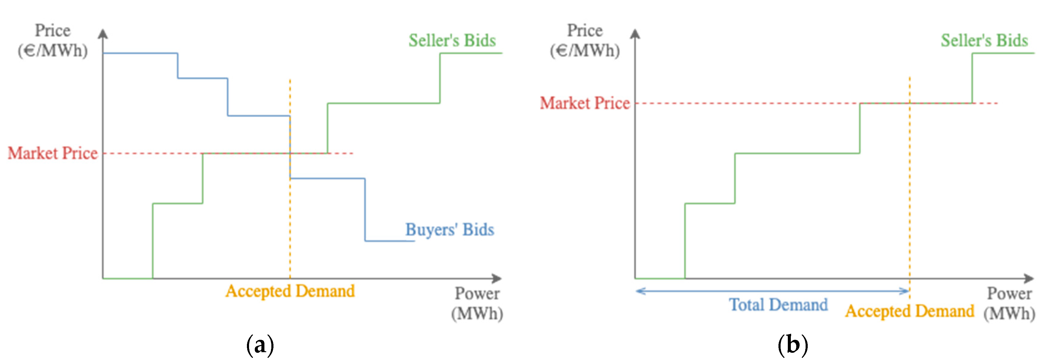
To show the application of our solution, we consider one hour of market operation (a session from 14:00 to 15:00), split into periods of 15 min, in which each player participates with buy or sell bids and, when desired, the respective constraints. The players will be bidding on an hour-ahead basis, meaning that this local market session will run in the hour before (between 13:00 and 14:00). The local market proposed is based on the symmetric market pool [35,36], where both buyers and suppliers can compete by submitting their bids.

The session starts with the aggregator sending the call for proposals for the next local market session. The players interested in participating submit their bids for each period and the desired constraints from 13:15 to 13:45.

Table 2. Payers’ bids for the local market hour-ahead session.

Player	Bids								Instant
	14:00		14:15		14:30		14:45
	kWh	EUR	kWh	EUR	kWh	EUR	kWh	EUR
House 1	0.1127	0.1392	0.1127	0.1103	0.1127	0.0987	0.1127	0.0959	13:40:29.266
House 2	0.2921	0.1211	0.2852	0.1659	1.1293	0.0985	2.5599	0.0982	13:39:53.629
House 3	0.4485	0.1104	0.2806	0.1183	0.6164	0.0979	0.2806	0.0974	13:16:34.193
House 4	−0.2303	0.1132	−0.2751	0.1092	−0.263	0.0974	−0.3623	0.0968	13:20:54.956
House 5	1.2121	0.1598	0.5244	0.1646	0.506	0.0985	0.7107	0.0959	13:19:02.981
House 6	1.0373	0.1609	0.4554	0.1388	0.8096	0.0985	0.0736	0.0972	13:15:59.810
House 7	0.2346	0.1738	2.093	0.1901	1.7526	0.0977	0.2576	0.096	13:42:55.789
House 8	−0.3854	0.1213	−0.4069	0.1118	−0.6145	0.0959	−0.6224	0.0987	13:33:27.166
House 9	0.8142	0.1597	0.8142	0.1766	0.6049	0.0977	0.6647	0.0972	13:31:01.235
House 10	0.0621	0.1827	0.0598	0.172	0.0552	0.0955	0.1173	0.0962	13:26:34.783
House 11	0.5244	0.1016	0.5589	0.1305	0.6762	0.0966	0.2806	0.0958	13:39:24.004
House 12	0	0	0	0	0	0	0.1058	0.0978	13:25:23.407
House 13	0.4255	0.0972	0.3036	0.1286	0.6578	0.0985	0.3565	0.0984	13:43:18.609
House 14	0.1725	0.1126	0.1771	0.1207	0.1794	0.0961	0.2691	0.0961	13:21:20.237
House 15	0.1909	0.1718	0.1817	0.1552	0.2047	0.095	0.2047	0.0975	13:23:38.991
House 16	0.5497	0.1542	0.5497	0.1277	0.5198	0.0979	0.5589	0.0977	13:40:11.062
House 17	0.1817	0.1768	0.1771	0.1784	0.3496	0.0966	0.2277	0.0973	13:34:18.168
House 18	0.5474	0.13	0.529	0.1672	0.2852	0.0977	0.3726	0.0983	13:44:53.266
House 19	0.299	0.1377	0.2921	0.1134	0.2921	0.0966	0.2737	0.097	13:25:00.754
House 20	0.1817	0.1072	0.1955	0.1742	0.1932	0.0957	0.2047	0.0986	13:31:39.420
House 21	−0.2499	0.1697	−0.9392	0.137	−0.1929	0.0968	−0.3825	0.0968	13:18:27.320
House 22	0.2438	0.1065	0.2346	0.1696	0.2438	0.095	0.2438	0.0964	13:24:34.370
House 23	−0.181	0.1745	−0.2355	0.192	−0.2014	0.0961	−0.1756	0.0979	13:26:29.464
Culture Hall	7.9245	0.1043	8.512	0.1406	10.499	0.28	9.427	0.1226	13:24:34.014
Library	−2.4055	0.0996	−0.3615	0.1135	−3.282	0.1214	−3.3615	0.2316	13:15:34.989
City Hall	−2.332	0.1394	−3.006	0.1134	−2.75	0.2471	−2.345	0.2431	13:31:11.450
Municipal Market	−1.987	0.0998	−1.8907	0.1134	−1.8507	0.2937	−1.127	0.2198	13:42:13.688

presents the considered local market players, their bids, and the instant at which the aggregator received each proposal. The golden color gradient identifies the prices ordered from the darkest (higher) to the lightest (lower). Likewise, the green gradient distinguishes the higher and lower demand energy, while the blue concerns the energy surplus.

When analyzing Table 2, it is possible to verify that all twenty-seven players decided to participate in the current hourly session. The instant the aggregator receives each proposal is important so that they can arrange the bids with equal prices by order of arrival. The bids with negative energy values are sell bids, while the positive energy values represent buy bids. In the current session, House 4, House 8, House 21, House 23, Library, City Hall, and Municipal Market all sell bids. These are all the available prosumers in the community. Prosumers calculate the difference between consumption and generation forecasts to determine the available surplus energy that they can offer in the market for each period. Since these prosumers depend on renewable generation, their generation is unstable. In this specific case, it depends on the solar radiation, time of day, and time of year. Thus, there are several situations in which generation is not enough to supply each player demand. In those situations, there is no surplus energy to be sold in the local market. Bid prices are defined strategically based on the base tariff of each player.

Table 3. Players’ base tariffs.

Player	Consumption Tariffs (EUR/kWh)				Generation Tariff (EUR/kWh)
	14:00	14:15	14:30	14:45
House 1 to House 23	0.1962		0.0988		0.0950
Culture Hall, Library, City Hall, Municipal Market	0.1445		0.3000

shows the generation and consumption tariffs contracted by each player.

When looking at Table 3, it is possible to see that both residential and public building players contract multi-hourly tariffs. Additionally, the generation tariff is constant for all prosumers during all day. These data are based on real tariff data, although the multi-hourly tariffs periods do not change at this specific time of day. The decision to change the tariff in the middle of the session aims to verify how the proposed local market behaves in this scenario. Through these tariffs, each player defined the prices for each period, keeping in mind that prices lower than the generation base tariff will not attract prosumers and prices higher than the base consumption tariff will not attract consumers. Prices defined as in between are used strategically by each player to reach their goals. Consumers want to minimize costs, while prosumers intend to maximize their profits. A different and complementary type of strategy is the use of (period/session) constraints in which—if they are not satisfied—players may decide not to participate in the market pool or to update their bids accordingly.

Table 4. Players’ session constraints.

Player	Maximum Cost		Minimum Income		Maximum Matched Energy (kWh)	Minimum Matched Energy (kWh)
	EUR	EUR/kWh	EUR	EUR/kWh
House 1	0.0437	0.0970
House 4					1.1000
House 8					2.0000	1.0000
House 23						0.6500
Library			0.9000	0.1000
M. Market			1.2040	0.1817	6.5000	3.5000

and

Table 5. Players’ period constraints.

Player	Maximum Matched Energy (kWh)				Minimum Matched Energy (kWh)
	57	58	59	60	57	58	59	60
House 1					0.1000	0.0900	0.1100	0.1000
House 8				0.6077
House 23					0.1500	0.2000
Culture Hall							8.0000
M. Market	1.9000	1.8000	1.8000	1.0000	1.0000	1.0000	1.0000	1.0000

present the constraints submitted in the current session and periods, respectively.

When inspecting Table 4 and Table 5, it is perceptible that the Library and House 4 players only submitted a session constraint, while the Culture Hall player submitted one restriction for period 59. The Municipal Market is the player that submitted all types of constraints (since it is a seller, it makes no sense for it to submit the Maximum Cost constraint). The House 1, House 8, and House 23 players also submitted their strategic constraints, trying to achieve their goals.

As explained in Section 3, the local auction-based market library receives these input data as an RDF KB file. The KB file, as well as the configuration file and the resource files, are available online (http://www.gecad.isep.ipp.pt/mdpi/energies/845690/), as well as the input and output files of the various symmetrical pool executions for test and proof purposes. To avoid distracting the reader from the purpose of this work, this case study will focus on describing the triggered local market constraints.

The system starts by querying it to get the ordered periods of the session and creates a temporary graph for each period. Next, it queries the graph of period 57 (dividing the day into periods of 15 min, from 14:00 to 14:15 is the period 57) to get the players’ demand and supply bids, ordered by price, to run the symmetrical algorithm. The output of the algorithm is added, afterwards, to the KB period’s graph. The next step is to apply the players’ constraints to the pool results. For this, the system queries the KB to get the suppliers’ and demanders’ constraints. These are ordered by bid price (ascending in the case of suppliers/descending in the case of demanders), time of arrival and priority, so that the players’ restrictions are applied in the same order as the pool bids. As presented above, for the period constraints, players can define a maximum and minimum matched energy amount. This starts by applying the suppliers’ constraints. The suppliers House 23 and Municipal Market submitted restrictions for period 57 (Table 5). House 23 did not trade in this period, while Municipal Market traded the total offered amount of energy, namely 1.987 kWh (Table 2). However, Municipal Market also defined a Maximum Matched Energy restriction at 1.9 kWh (Table 5). By applying this constraint, the Municipal Market bid is reduced to 1.9 kWh and the market pool rerun for period 57. As explained in Section 3.1, this restriction does not remove the player from the market pool but reduces the offered amount of energy to the constraint value.

The system reruns period 57, and no other restriction is triggered. It runs the market pool for period 58 by following the same process, but on a different graph. Once again, the Municipal Market triggers the Maximum Matched Energy constraint, this time set at 1.8 kWh, being the traded energy amount 1.8907 kWh. Its bid is updated by the rule, and the market reruns for period 58. Again, no other constraints were triggered. The system continues its execution by running the period 59 pool. This time, the Culture Hall is removed from the market pool because of the Minimum Matched Energy constraint, set at 8 kWh. Its traded amount was 7.3038 kWh. After removing the Culture Hall player from the period’s pool, the system executes it again, and this time no more issues are found. The system continues for period 60. In this period, the Maximum Matched Energy restriction, set by House 8, is triggered. House 8 defined a maximum value of 0.6077 kWh. However, the pool result was 0.6224 kWh. As in periods 57 and 58, the rule reduces the bid amount of energy, and the market continues smoothly.

After the execution of all periods ends, the system updates the KB with the players’ aggregated results, namely the total transacted energy, the total bought/sold energy, and the session’s total cost/income. Next, the system queries the KB to get the session’s constraints ordered by the time of arrival and priority. In this case, the supply and demand bids are not discriminated, since a player can buy in one period and sell in the next one. The first rule to trigger is the constraint set by the Library player. This player is removed from the session because of the Minimum Income constraint set at EUR 0.9, and the total income of this player was EUR 0.2806. The Minimum Income constraint states that if the player’s total income or the price per kWh is below a predefined amount, then he must be removed from the pool since he does not want to participate if those conditions are not met. Due to this constraint, Library player is removed from this local market session, not trading in any period, as illustrated in Figure 3.

The session is rerun, and this time there are no period restrictions triggered. In turn, the Maximum Matched Energy session constraint triggers for the House 4 player. This player set this constraint at 1.1 kWh. However, it trades at 1.1307 kWh in the complete session, which removes it from the market pool. The session is rerun. This time, the session’s Minimum Matched Energy constraint triggers for player House 23. This player traded 0.377 kWh but has set a minimum value of 0.65 kWh for the session. As such, House 23 is removed from the session’s pool. The session reruns and the Maximum Matched Energy restriction set by House 8 removes it from the pool. House 8 set a maximum of 2 kWh for the session and trades at 2.0145 kWh.

In the next run, the Maximum Cost rule is triggered for player House 1. This player defined a maximum cost of EUR 0.0437 and a maximum price per kWh of EUR 0.097. In this market session, the House 1 player only traded in period 59, 0.1127 kWh for EUR 0.0974 per kWh. The total cost is EUR 0.0437, which is accepted by the rule defined by House 1. However, the price per kWh is higher than the EUR 0.097 determined in the constraint. The market pool reruns again. This time, the Municipal Market player is removed from the pool due to the Minimum Income constraint. The Municipal Market set a minimum income of EUR 1.204 and at least EUR 0.1817 per kWh. This player only achieves an income of EUR 0.5115 and is removed from the pool. The seventh run of the session pool concludes the local market execution. No more constraints are triggered, and the system returns the final results.

Table 6. Local market session aggregate results.

Energy Volume (kWh)	Price Volume (EUR)	Minimum Price (EUR/kWh)	Maximum Price (EUR/kWh)	Average Price (EUR/kWh)
6.8526	0.9221	0.0974	0.1394	0.1181

presents the aggregated results of the local market session.

The total amount of traded energy in the local market was 6.8526 kWh, with a monetary volume of EUR 0.9221. The minimum price of the session was of EUR 0.0974 in period 59. Period 57 presented the highest price of EUR 0.1394. The average price of the session was EUR 0.1181. Figure 4a shows the players’ transacted energy in each period, and (b) the period’s total traded energy, the market prices, and the number of players dispatched.

When analyzing Figure 4a, it can be seen that only thirteen players were able to trade in this session (less than 50%). From these, only two players are prosumers since the remaining players were removed due to their constraints. These prosumers are identified by the negative energy, as in Table 2. In Figure 4b, it can be seen that the first two sessions had more traded energy and dispatched players than the next two. On one hand, the first two periods had more available energy to trade; on the other, the player with more energy surplus (Municipal Market) was removed from the session due to their constraints.

To demonstrate the ease of changing the rules of the local electricity market, without the need to reprogram and recompile the system, we will add a new constraint. The new restriction is a new version of the Minimum Income rule that removed the Library player from the market session (see Figure 3). The difference between this constraint and the new one is that, in the original proposal, both the total income and price per kWh must be higher or equal to the values predetermined by the player, while, in the second version, if one of the values is higher than those determined by the player, then the rule will not be triggered and the player will not be removed from the pool. Figure 3 illustrates that, although the Library player achieved a price per kWh higher than the minimum value accepted, he was removed from the market session due to not achieving the minimum total income defined. With the new version of this rule, the Library player will not be removed and will be able to trade in the market session.

The first step is to add the new constraint to the semantic model (http://www.gecad.isep.ipp.pt/mdpi/energies/845690/#onto-lmo-v2). Since the constraint’s attributes will be the same as the MinimumIncome class defined in Table 1, the new rule can be simply defined as a subclass of MinimumIncome, i.e., MinimumIncomeV2 extends MinimumIncome, inheriting its attributes, namely the properties hasTotalIncome and pricePerkWh, as well as the priority inherited from the class Constraint. Afterwards, the new constraint template must be added to the configuration file (http://www.gecad.isep.ipp.pt/mdpi/energies/845690/#in-conf-v2). When looking at Listing 1, the difference between MinimumIncome and MinimumIncomeV2 is in line 36, where the operator || (OR) is replaced by the operator AND (&&). Finally, the instance of the Library player in the KB file (http://www.gecad.isep.ipp.pt/mdpi/energies/845690/#in-kb-v2) is also updated to use the MinimumIncomeV2 constraint instead of MinimumIncome.

After the first iteration of the execution of the market session, it is possible to verify that the Library player was not excluded from the market pool. His results were the same; however, the MinimumIncomeV2 constraint did not trigger since the price per kWh is higher than the minimum value predetermined by the player. Figure 5 illustrates this scenario.

The above example has the purpose of showing the simplicity and flexibility of the system when adding a new rule. On the other hand, one could update the MinimumIncome template to accomplish the constraint defined by MinimumIncomeV2. This flexibility is of great value when the main purpose of the system is to enable the study of different possibilities.

The developed system is agnostic to the constraint rules configured, as well as to the semantic models used. Their use is an advantage when developing systems that evolve rapidly since, when a rule must be updated, or added, there is no need to reprogram the system. To update a rule, the developer will only need to rewrite it in the configuration file. To add a new constraint, the developer must add it to the semantic model (as a subclass of Constraint class) and add the respective SPARQL rule to the configuration file. Finally, it is also possible to use a different semantic model. For such, it is only necessary to update the resource files in order to get the required data for the system to solve the local auction-based market pool.

5. Conclusions

Energy markets are constantly evolving due to the large-scale implementation of RES and DG in response to the environmental targets imposed worldwide. Recent directives invest in the design, development, and implementation of local electricity markets to fulfill these targets, taking advantage of the increased use of RES and DG to keep the grid balanced and avoid the use of fossil fuels to produce electricity. Several works propose varied solutions to solve local electricity markets for different purposes.

This work proposed the use of constrained bid transactions in local electricity markets. To this end, it presents the design and development of a library that takes advantage of semantic web technologies to be flexible and agnostic to the data model and business rules. In this way, it avoids the need to reprogram the system any time a rule is added, removed, or updated. The solution proposed had in mind the constant evolution of the markets, allowing its users to spend more time on studying and testing different market alternatives than on programing a new alternative. The focus was given to distributed generation, so the respective owners can profit better from their participation in local markets, increasing the amount of energy negotiated.

This document provides a background overview of auction-based electricity market types, local market bid constraints, and the advantages of using ontologies and semantic web technologies instead of coding data models and business rules, as well as the solution’s architecture, the proposed constraints, the application ontology, and the rules’ SPARQL templates. The case study illustrates a scenario based on real data executed in the proposed solution, describing the bid constraints triggered. It demonstrates the advantage of using semantic web technologies in the development of solutions toward constantly evolving domains such as the electricity market. A community of 27 consumers was used in the case study, showing the effectiveness of the proposed methodology. The next steps are to improve the players’ constraints and design and to implement aggregator restrictions, while considering the grid constraints. The players’ constraints can be improved by suggesting new ones or by updating the ones proposed, regarding, for example, the players’ targets and preferences in a complete day, in the total results of all the sessions. To achieve this, studies and experiments must be performed to analyze how these may or may not benefit the players that use them. A scalability study will also be performed to enable the use of the proposed solution in larger communities.