Abstract
The fastest-growing renewable source of energy is solar photovoltaic (PV) energy, which is likely to become the largest electricity source in the world by 2050. In order to be a viable alternative energy source, PV systems should maximise their efficiency and operate flawlessly. However, in practice, many PV systems do not operate at their full capacity due to several types of anomalies. We propose tailored algorithms for the detection of different PV system anomalies, including suboptimal orientation, daytime and sunrise/sunset shading, brief and sustained daytime zero-production, and low maximum production. Furthermore, we establish simple metrics to assess the severity of suboptimal orientation and daytime shading. The proposed detection algorithms were applied to a set of time-series of electricity production in Portugal, which are based on two periods with distinct weather conditions. Under favourable weather conditions, the algorithms successfully detected most of the time-series labelled with either daytime or sunrise/sunset shading, and with either sustained or brief daytime zero-production. There was a relatively low percentage of false positives, such that most of the anomaly detections were correct. As expected, the algorithms tend to be more robust under favourable rather than under adverse weather conditions. The proposed algorithms may prove to be useful not only to research specialists, but also to energy utilities and owners of small- and medium-sized PV systems, who may thereby effortlessly monitor their operation and performance.
1. Introduction
The concentration of greenhouse gases (GHGs) in the Earth’s atmosphere has been steadily increasing since the Industrial Revolution [1] and has thereby contributed to global warming over the last two centuries [2,3,4]. This trend is primarily due to human activity, where the energy sector has become a significant driver of GHG emissions [5]. Indeed, if current practices in energy production are to be maintained, global temperature is expected to increase as much as 6 °C above pre-industrial levels by 2050 [6]. There is therefore an urgent need to shift from carbon-intensive to sustainable and renewable energy sources, and thereby reduce GHG emissions to limit global warming to 1.5 °C by 2050 [7].
Solar photovoltaic (PV) energy is perhaps the most promising and fastest-growing renewable source of energy, and it is poised to become the world’s largest source of electricity by 2050 [5]. Hence, PV systems have great potential to reduce the current dependence on carbon-intensive sources of energy, and progress has been made to enhance their efficiency. In fact, solar cell efficiency has increased from about 5% to over 40% over the last 60 years [8], yet current efficiency levels are rather low compared to those of alternative sources of energy. PV systems should ideally operate seamlessly without anomalies to maximise efficiency and remain a viable alternative energy source. In reality, however, several kinds of anomalies may occur that prevent PV systems from operating at their full capacity. Thus, it is important to monitor the activity of PV systems, so that these anomalies can be detected and repaired to ensure maximum efficiency [9,10,11,12].
Anomaly detection in PV systems can be performed using several methods, ranging from classical statistics to data mining and machine learning [13,14]. Although such methods may be well suited to detect anomalies in PV systems, they typically require data that might not be readily available for anomaly detection. In particular, several methods of anomaly detection are based not only on PV system production, but also on environmental data such as solar irradiation or temperature (e.g., [15,16,17,18,19]). Alternatively, ref. [20] proposes a method of anomaly detection in PV systems based on inferential statistical tools, which does not require environmental data. However, this method is designed strictly for anomaly detection in PV systems, and thus it is not devised to identify and distinguish several types of anomalies.
We address this problem by developing anomaly detection algorithms that indicate whether and why a given PV system is not operating properly, and propose simple metrics to estimate anomaly severity. Specifically, five algorithms tailored to detect PV system anomalies are evaluated, and they also identify the cause of such anomalies: daytime zero-production, low maximum production, daytime shading, sunrise/sunset shading, and suboptimal orientation. Importantly, the algorithms are based on simple rules that solely require the PV system production as input data for anomaly detection. Although PV systems are becoming increasingly sophisticated and currently allow for the monitoring of environmental parameters, a significant share of PV systems still does not offer this possibility and may therefore benefit from the widely applicable algorithms that are proposed. These algorithms may prove useful not only to research specialists, but also to energy utilities and owners of small- and medium-sized PV systems, who may thereby effortlessly monitor their operation and performance.
The usefulness of the proposed methods is demonstrated with time-series of electricity production in Portugal, which were acquired for two periods with contrasting weather conditions. The majority of PV systems analysed in this study are small solar panels used for domestic purposes, and therefore similar in their structure. Furthermore, the geographical distribution of PV systems is restricted to the continental territory of Portugal, such that weather conditions (e.g., daytime period, air temperature) are regionally similar.
2. PV System Anomalies: An Overview
Despite their potential to offer a clean and inexhaustible source of energy, PV systems often operate suboptimally due to several kinds of anomalies. Two major types of PV system anomalies are distinguished: (1) internal PV system faults, which originate from the PV system itself, and (2) external factors, which do not originate from the PV system and yet impair its electricity production. Although this categorization of PV system anomalies is arbitrary, it facilitates the distinction between anomalies that largely result in daytime zero-production (i.e., internal faults) and those that result in reduced nonzero production (i.e., external factors). A brief overview of these two major types of PV system anomalies is provided below and highlights their impact on electricity production.
2.1. Internal PV System Faults
Typical PV system faults include component failure, system isolation due to maintenance work, inverter shutdown due to power cuts or variations in grid voltage, and inverter dropout due to maximum power point tracking (MPPT; [11]). Table 1 presents a short description of these common PV system faults and indicates their impact on electricity production. PV systems consisting of a single module are considered in Table 1, which therefore does not include faults in PV systems comprising several modules (e.g., failure of single PV modules and module mismatch). Most PV system faults analysed by [11] lead to episodes of brief or sustained zero-production, whereas nonzero production occurs only in case of inverter dropout.

Table 1.
Description of photovoltaic (PV) system faults and their impacts (Adapted from [11], Elsevier: 2010).
2.2. External Factors Impairing PV System Performance
There are other factors besides PV system faults, which are external to PV systems and prevent the generation of maximum electrical power (Table 2). High wind speed may either increase or decrease power generation [21]. Specifically, high wind speed increases the efficiency of PV systems by reducing relative humidity, whereas it can decrease efficiency by scattering dust, and causing shading. Vandalism and theft also affect power generation in PV systems, although their impact remains poorly studied [22].
Table 2.
External factors impairing electricity production.
3. Methods
3.1. Algorithms for Anomaly Detection
We developed five algorithms for anomaly detection, which also allow for the identification of several types of anomalies: daytime zero-production, low maximum production, daytime shading, sunrise/sunset shading, and suboptimal orientation. That is, the algorithms are designed to pinpoint the cause of production anomalies in PV systems, so that these production anomalies may be readily solved. The proposed algorithms are summarised in Figure 1 and detailed in the following sections.
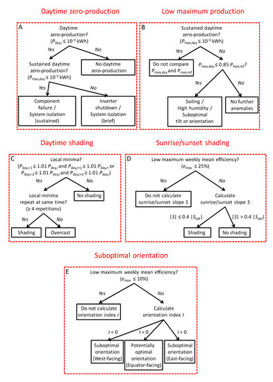
Figure 1.
Overview of the algorithms for anomaly detection. (A) Daytime zero-production algorithm; (B) low maximum production algorithm; (C) daytime shading algorithm; (D) sunrise/sunset shading algorithm; and (E) suboptimal orientation algorithm.
3.1.1. Daytime Zero-Production
Anomalies leading to daytime zero-production include most of the internal PV system faults shown in Table 1. It is assumed that time-series with daytime zero-production have at least one daytime observation where production, Pday,i, is sufficiently close to zero (i.e., where Pday,i ≤ 10−3 kWh; see Figure 1A). That is, the threshold for daytime zero-production has been set at 10−3 kWh. Although this is an arbitrary value, the sensitivity of the algorithms to changes in the threshold for zero-production was tested, and we found that a threshold of 10−3 kWh is the most satisfactory. Specifically, lower thresholds result in lower detection rates of daytime zero-production, whereas higher thresholds result in higher percentage of false daytime zero-production detections.
To determine the daytime period, we propose to first calculate the hour angle, ωs, at which sunrise (−ωs) and sunset (ωs) occur:
where ϕ is the latitude at which the PV system is located and δ is the Sun’s declination angle:
which varies daily throughout the year, where n is the day number. Subsequently, the sunrise/sunset hour angle is converted to decimal hours using the equation of time [28], and the daytime period is defined as the following interval:
where tSR and tSS are the sunrise and sunset time in decimal hours, respectively, and offset = 2.5 h prevents the false detection of daytime zero-production (e.g., due to sunrise/sunset shading; see below). The offset has been defined at 2.5 h after investigating the sensitivity of the algorithms to this parameter, and finding that their performance is most satisfactory at this value. Specifically, shorter offsets result in more false detections of daytime zero-production, whereas longer offsets result in lower detection rates of daytime zero-production.
If a given time-series has episodes of daytime zero-production, then this algorithm determines whether such episodes are sustained or brief. According to Table 1, sustained daytime zero-production can result from component failure or sustained system isolation, whereas brief daytime zero-production can result from inverter shutdown or brief system isolation. On the one hand, sustained daytime zero-production is considered to last at least one day, such that the maximum production during daytime on a given day, Pmax,day, is sufficiently close to zero (i.e., Pmax,day ≤ 10−3 kWh). On the other hand, brief daytime zero-production is considered to last less than one day, such that the maximum production on a given day during the daytime is sufficiently higher than zero (i.e., Pmax,day > 10−3 kWh).
3.1.2. Low Maximum Production
It is assumed that low maximum production may result from high humidity, soiling or suboptimal tilt/orientation of the PV system, all of which incur substantial output losses (Table 2). These anomalies contrast with high temperature, which incurs relatively small output losses of up to 15%. To detect low maximum production (Figure 1B), we propose an algorithm that determines whether maximum production on a given day, Pmax,day, is sufficiently higher than zero and substantially lower than a reference value, Pmax,ref, so that 10−3 < Pmax,day ≤ 0.85 Pmax,ref. That is, low maximum production is detected whenever output losses are greater than 15%, in which case PV system performance is likely impaired by high humidity, soiling or suboptimal tilt/orientation.
The reference value of maximum production corresponds to a standard PV system capacity (i.e., 62.5 kWh, 125 kWh, 187.5 kWh, 250 kWh, and so on for a period of 15 min), and is calculated based on the historical maximum of production. Specifically, the reference value is the closest standard capacity above the historical maximum, where the historical maximum is a median of the 25 highest observations for a given PV system over the analysed five-week period. For example, if maximum production on a given day is 90 kWh and the reference value is 125 kWh, then the PV system is assumed to be operating substantially below capacity (i.e., at 72%) on that day.
3.1.3. Daytime Shading
To detect episodes of shading during the daytime, we propose an algorithm that determines whether a given time-series shows regular local minima (Figure 1C). It is assumed that time-series with local minima have at least one observation that is a local minimum. To ensure the detection of consecutive local minima and avoid the detection of negligible local minima, we adopt a somewhat more stringent definition of a local minimum than it is common. More specifically, the daytime observation Pday,i is considered a local minimum if the production of either both its nearest neighbours, Pday,i−1 and Pday,i+1, or both its second-nearest neighbours, Pday,i−2 and Pday,i+2, are at least 1% higher than Pday,i.
If a time-series has local minima, then this algorithm determines whether such local minima occur regularly (i.e., at least four days in a week) at a specific time of the day. This repetitive pattern is likely due to shading, which causes a recurrent drop in production at a particular time of the day. Local minima that otherwise occur irregularly are assumed to result from adverse weather conditions (e.g., overcast or rainy weather).
3.1.4. Sunrise/Sunset Shading
Shading may occur not only during daytime, but also at sunrise/sunset. Shading at sunrise/sunset can be readily detected if the slope of production at sunrise/sunset is substantially less steep than expected. To detect episodes of sunrise/sunset shading, we developed an algorithm that compares the steepness of the observed slope of production at sunrise/sunset with that of an optimum slope of production (Figure 1D).
To obtain an optimum slope of production at sunrise/sunset, the optimum PV system efficiency is modelled under ideal weather conditions, eopt. Specifically, the hourly solar irradiation on a PV system is first estimated based on [29], assuming that the PV system has optimum tilt/orientation and taking into account its geographical location. Subsequently, the estimated hourly solar irradiation is used to simulate the efficiency of a model PV system as described by [30]. We refer to Appendix A for a detailed description of the estimation of hourly solar irradiation, and to Appendix B for a detailed description of the estimation of optimum PV system efficiency.
To calculate the observed slope of production at sunrise/sunset, we first draw a curve of weekly mean efficiency of the PV system, e. This curve is obtained by calculating the ratio between the weekly average of electricity production throughout the day, and the reference value of maximum production. Subsequently, the slope of weekly mean efficiency is calculated at sunrise and sunset, SSR and SSS, respectively:
where eSR (eSS) is the weekly mean efficiency at sunrise (sunset), and eSR+offset (eSS−offset) is the weekly mean efficiency after sunrise (before sunset). These observed slopes of weekly mean efficiency are then compared with optimum slopes, Sopt,SR and Sopt,SS, obtained from the PV system model:
where eopt,SR and eopt,SS are the optimum efficiency at sunrise and sunset, respectively. Thus, sunrise and sunset shading are detected if observed slopes are at most 40% as steep as optimum slopes (i.e., if |SSR| ≤ 0.4 |Sopt,SR| and |SSS| ≤ 0.4 |Sopt,SS|, respectively). We investigated the sensitivity of the algorithm to changes in this steepness threshold, and found that a steepness threshold either lower or higher than 40% impairs algorithm performance.
3.1.5. Suboptimal Orientation
PV systems with suboptimal orientation are characterised not only by substantial losses in electricity production (Table 2), but also by a temporal mismatch between observed weekly mean efficiency and optimum efficiency (Figure 1E and Figure 2). The extent to which the orientation of a PV system deviates from optimum conditions is determined by calculating its orientation index at sunrise and sunset, ISR and ISS, respectively:
where topt,SR is the moment when optimum efficiency increases to 10% of maximum optimum efficiency, and tSR is the moment when weekly mean efficiency increases to 10% of maximum optimum efficiency. Conversely, topt,SS is the moment when optimum efficiency drops to 10% of maximum optimum efficiency, and tSS is the moment when weekly mean efficiency drops to 10% of maximum optimum efficiency.
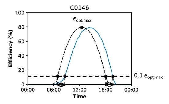
Figure 2.
Estimation of orientation index from a weekly mean efficiency curve. The blue curve indicates the observed weekly mean efficiency, and the black dashed curve indicates the simulated efficiency under optimum conditions. Black solid circles denote the optimum efficiency maximum, eopt,max, and points where observed and optimum efficiency increase or decrease to 10% of the optimum efficiency maximum.
The orientation index of a given PV system simply corresponds to the average of its sunrise and sunset orientation indices:
Thus, the orientation of a PV system is assumed to be equator-facing and potentially optimal if I = 0. Conversely, the orientation of a PV system is assumed to be suboptimal if I ≠ 0, and considered to be west-facing if I < 0 and east-facing if I > 0.
3.2. Estimation of Anomaly Severity
Although the detection algorithms described above can be used to identify several types of anomalies, these algorithms do not measure the severity of anomalies. However, anomaly severity is important to determine, because it indicates the extent to which a given anomaly impairs PV system performance. To address this issue, we introduce simple metrics that quantify the severity of two anomalies, namely daytime shading and suboptimal orientation.
3.2.1. Daytime Shading Magnitude and Length
In case daytime shading events are detected in a time-series, the severity of daytime shading is measured by calculating its magnitude and length. To this end, we first draw a curve showing the weekly mean efficiency of a PV system, e. Typically, PV systems affected by daytime shading will have weekly mean efficiency curves with one local minimum, emin, and two local maxima, emax,1 and emax,2 (Figure 3). Subsequently, the weekly mean efficiency curves are used to determine the magnitude and length of daytime shading. On the one hand, shading magnitude, M, is calculated as the standardised difference between the expected efficiency in the absence of daytime shading, eexp, and the observed local efficiency minimum:
where the expected efficiency is estimated by linear regression through the two local efficiency maxima (Figure 3A). On the other hand, shading length, L, is calculated as the time interval between the moment of one of the local efficiency maxima, tmax,1 or tmax,2, and the moment when observed efficiency matches expected efficiency, texp (Figure 3B):
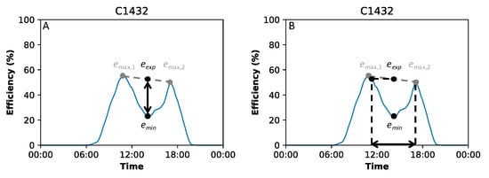
Figure 3.
Estimation of daytime shading severity from a weekly mean efficiency curve. (A) Shading magnitude, and (B) shading length. Blue curves indicate the observed weekly mean efficiency. Black solid circles denote the local efficiency minimum, emin, and the expected efficiency in the absence of daytime shading, eexp. Gray solid circles denote the two local efficiency maxima, emax,1 and emax,2, associated with daytime shading.
We propose this definition of shading length, instead of simply calculating tmax,2 − tmax,1, because it prevents overestimation in some cases. Specifically, daytime shading may briefly occur before or after electricity production peaks, such that the time interval tmax,2 − tmax,1 is actually much longer than the shading itself. We found that Equation (12) effectively reduces this overestimation.
Hence, the severity of daytime shading is determined by calculating its magnitude and length, such that severe daytime shading events are assumed to have a larger magnitude and last for more extended periods. More specifically, the severity of daytime shading is classified into three different categories: mild shading if M ≤ 15% and L ≤ 1.5 h, severe shading if M ≥ 30% and L ≥ 3 h and moderate shading otherwise.
3.2.2. Orientation Index
Similar to daytime shading, the severity of suboptimal orientation is classified into three different categories, which depend on the orientation index described above. Hence, a PV system is assumed to have mildly suboptimal orientation if 0 h < |I| ≤ 1 h, moderately suboptimal orientation if 1 h < |I| ≤ 2 h, and severely suboptimal orientation if |I| > 2 h.
3.3. Algorithm Performance Indicators
We manually annotated time-series with sustained or brief daytime zero-production, daytime shading and sunrise/sunset shading, in order to evaluate the performance of the anomaly detection algorithms. Subsequently, two indicators were used to measure the performance of the detection algorithms for these anomalies. First, the detection rate, DR, was calculated as the ratio between the number of time-series correctly detected as anomalous by a given algorithm, Correct, and the total number of time-series annotated with a given anomaly, Annotated:
Second, the percentage of false positives, FP, was calculated as the ratio between the number of time-series incorrectly detected as anomalous by a given algorithm, Incorrect, and the total number of time-series detected as anomalous by that algorithm, Total:
where Incorrect = Total − Correct. In other words, FP is the proportion of time-series identified by a given detection algorithm as anomalous, which are in fact not annotated as such. Therefore, it is assumed that the performance of a given detection algorithm depends on its detection rate (also known as recall or sensitivity; [31]) and percentage of false positives, such that robust algorithms will have high detection rate and produce a low percentage of false positives.
We note that time-series annotation is particularly difficult for low maximum production and suboptimal orientation, because we do not have prior knowledge about the maximum capacity and orientation of the PV systems. Thus, we did not determine the detection rate and percentage of false positive detections of these two algorithms.
3.4. Electricity Time-Series
To assess the performance of the proposed anomaly detection algorithms, a dataset including 1676 univariate time-series of electricity production in Portugal was analysed. Each time-series corresponds to a differently located PV system, and consists of electricity production measurements recorded every 15 min over several months to years (Figure 4). This dataset was used to test algorithms of anomaly detection and metrics of anomaly severity, as described below.
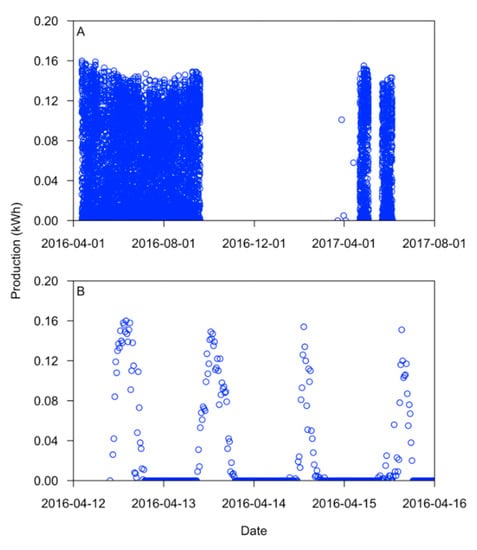
Figure 4.
Example of a time-series of electricity production analysed in this study. (A) Complete time-series, and (B) an excerpt from this time-series showing the first four days of electricity production.
Time-series for two short periods of five weeks with contrasting weather conditions were analysed, and anomaly detection was performed on the last week of these two periods. Specifically, we performed anomaly detection over the week of 1 to 7 August 2016, which was particularly favourable for PV system activity, and the week of 18 to 24 November 2016, which was particularly adverse for PV system activity. For simplicity, it is assumed that the daytime period is the same for all PV systems analysed in this study, and perform anomaly detection using the daytime period in Lisbon for 1 August 2016, and for 18 November 2016.
Several time-series have erroneous values or missing values, which are due to communication problems and preclude a proper analysis of the data. Therefore, anomaly detection was only performed on time-series that do not have erroneous values, which were detected as nonzero production levels recorded during night-time (i.e., between 00:00 and 04:00). Furthermore, time-series that are empty for either one of the whole two five-week periods of analysis were discarded. Hence, anomaly detection was performed on both complete and incomplete time-series, and a measure of accuracy was used to determine the reliability of anomaly detection. In particular, the accuracy of anomaly detection corresponds to the ratio between the number of observations in a given time-series, and the maximum possible number of observations that time-series can have. For illustration purposes, figures shown in the Results section correspond to complete time-series that were 100% accurate for anomaly detection. Data pre-processing yielded 407 eligible time-series for the favourable week in August, and 886 eligible time-series for the adverse week in November.
Hourly solar irradiation and the resulting PV system efficiency were estimated during 1 August 2016, and 18 November 2016, assuming that the PV system has optimum tilt/orientation and is located in Lisbon.
4. Results and Discussion
4.1. Algorithm Performance under Favourable Weather Conditions
4.1.1. Anomaly Detection
The algorithms developed in this study readily detected several types of anomalies under favourable weather conditions (Figure 5). First, 31 PV systems were detected with sustained daytime zero-production anomalies (Figure 5A), and 21 PV systems with brief daytime zero-production anomalies (Figure 5B). Following the time-series annotation, 27 PV systems were identified with sustained daytime zero-production and 31 PV systems with brief daytime zero-production. The detection rate of the algorithm for sustained and brief daytime zero-production was therefore 96% (16% false positives) and 61% (9.5% false positives), respectively.
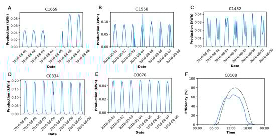
Figure 5.
Examples of photovoltaic (PV) systems detected with production anomalies under favourable weather conditions. (A) PV system with sustained daytime zero-production; (B) PV system with brief daytime zero-production; (C) PV system with daytime shading; (D) PV system with sunrise and sunset shading; (E) PV system with low maximum production; and (F) PV system with suboptimal orientation.
Second, the daytime shading algorithm detected 11 PV systems with regular local minima (Figure 5C), whereas the time-series annotation identified 17 PV systems with daytime shading. As a result, the detection rate of the daytime shading algorithm was 65%, and this algorithm did not produce any false positives. Moreover, the sunrise/sunset shading algorithm detected 35 PV systems with sunrise shading and 98 PV systems with sunset shading (Figure 5D), whereas the time-series annotation identified 53 PV systems with sunrise shading and 71 PV systems with sunset shading. Thus, the detection rate of the algorithm for sunrise and sunset shading was 57% (14% false positives) and 96% (31% false positives), respectively.
Third, the algorithms for low maximum production and suboptimal orientation detected 263 PV systems and 333 PV systems, respectively, with each type of anomaly (Figure 5E,F).
4.1.2. Anomaly Severity for Daytime Shading
To investigate daytime shading severity, the shading magnitude and length of the 11 PV systems correctly detected by the algorithm were calculated (Table 3). Shading magnitude varies considerably among PV systems and ranges from M = 7.9% to M = 59.8%. In other words, the local minima of weekly mean efficiency of the PV systems caused drops between 7.9% and 59.8% relative to the expected efficiency in the absence of shading. Similarly, shading length also varies considerably among PV systems and ranges from L = 0.75 h to L = 5.75 h.
Table 3.
Photovoltaic (PV) systems correctly detected with daytime shading under favourable weather conditions, and their respective shading magnitude, shading length and shading severity.
The shading magnitude and length of each PV system should be considered together, so that shading severity can be assessed. Thus, PV systems mildly affected by daytime shading will have low shading magnitude and short shading length, whereas PV systems severely affected by daytime shading will have high shading magnitude and long shading length. Figure 6 shows the contrast between electricity production and weekly mean efficiency of a PV system with mild daytime shading (Figure 6A,C), and those of a PV system with severe daytime shading (Figure 6B,D).
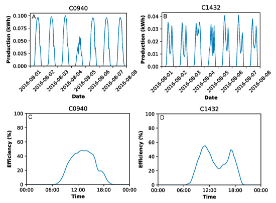
Figure 6.
Two photovoltaic (PV) systems with contrasting daytime shading severity. Time-series of electricity production for (A) a PV system with mild daytime shading, and (B) a PV system with severe daytime shading. Weekly mean efficiency curves for (C) a PV system with mild daytime shading, and (D) a PV system with severe daytime shading.
4.1.3. Anomaly Severity for Suboptimal Orientation
To investigate whether a given PV system has proper orientation, its orientation index was calculated (Figure 7). Similar to daytime shading magnitude and length, the orientation index varies considerably among PV systems and ranges from I = −5 h to I = 2 h. That is, the orientation index varies between negative and positive values, indicating that the weekly mean efficiency of PV systems with suboptimal orientation (i.e., with I ≠ 0 h) can be either lagging or leading, relative to the optimum efficiency curve.
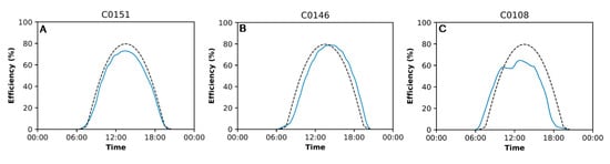
Figure 7.
Weekly mean efficiency curves of three photovoltaic (PV) systems with contrasting orientation index. (A) PV system with an orientation index of I = 0 h; (B) PV system with negative orientation index (I = –0.625 h); and (C) PV system with positive orientation index (I = 1.125 h). Blue curves indicate the observed weekly mean efficiency, and black dashed curves indicate the simulated efficiency under optimum conditions.
From the 353 PV systems eligible for orientation analysis, 20 PV systems have an orientation index of I = 0 h (Figure 7A), which indicates a potentially optimal orientation towards the equator. Therefore, the majority of PV systems appear to have suboptimal orientation. Specifically, 131 PV systems have a negative orientation index and are potentially west-facing (Figure 7B), whereas 202 PV systems have a positive orientation index and are potentially east-facing (Figure 7C).
4.2. Algorithm Performance Under Adverse Weather Conditions
4.2.1. Anomaly Detection
Similar to the anomaly detection under favourable weather conditions, the algorithms developed in this study also detected several types of anomalies under adverse weather conditions (Figure 8). First, 58 PV systems were detected with sustained daytime zero-production anomalies (Figure 8A), and 216 PV systems with brief daytime zero-production anomalies (Figure 8B). Following the time-series annotation, 49 PV systems were identified with sustained daytime zero-production and 143 PV systems with brief daytime zero-production. The detection rate of the algorithm for sustained and brief daytime zero-production was therefore 100% (16% false positives) and 67% (56% false positives), respectively.
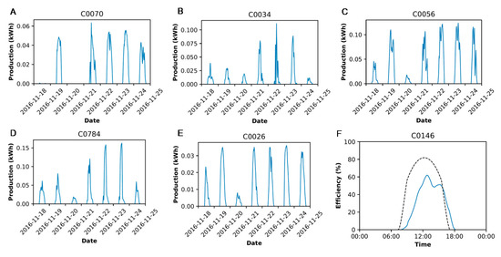
Figure 8.
Examples of photovoltaic (PV) systems detected with production anomalies under adverse weather conditions. (A) PV system with sustained daytime zero-production; (B) PV system with brief daytime zero-production; (C) PV system with daytime shading; (D) PV system with sunrise and sunset shading; (E) PV system with low maximum production; and (F) PV system with suboptimal orientation.
Second, the daytime shading algorithm detected 61 PV systems with regular local minima (Figure 8C), whereas the time-series annotation identified 26 PV systems with daytime shading. As a result, the detection rate of the daytime shading algorithm was 69% (71% false positives). Moreover, the sunrise/sunset shading algorithm detected 589 PV systems with sunrise shading and 373 PV systems with sunset shading (Figure 8D), whereas the time-series annotation identified 415 PV systems with sunrise shading and 134 PV systems with sunset shading. Thus, the detection rate of the algorithm for sunrise and sunset shading was 91% (35% false positives) and 78% (72% false positives), respectively.
Third, the algorithms for low maximum production and suboptimal orientation detected 643 PV systems and 796 PV systems, respectively, with each type of anomaly (Figure 8E,F).
4.2.2. Anomaly Severity for Daytime Shading
The shading magnitude and length of the 16 PV systems correctly detected by the algorithm were calculated (Table 4). Similar to the analysis under favourable weather conditions, shading magnitude varies considerably among PV systems and ranges from M = 0.6% to M = 60.7%. In other words, the local minima of weekly mean efficiency of the PV systems caused drops between 0.6% and 60.7% relative to expected efficiency in the absence of shading. Similarly, shading length also varies considerably among PV systems and ranges from L = 0.75 h to L = 3.25 h.
Table 4.
Photovoltaic (PV) systems correctly detected with daytime shading under adverse weather conditions, and their respective shading magnitude, shading length and shading severity.
4.2.3. Anomaly Severity for Suboptimal Orientation
The orientation index varies considerably among PV systems under adverse weather conditions and ranges from I = −4 h to I = 1.125 h. From the 813 PV systems eligible for orientation analysis, 17 PV systems have an orientation index of I = 0 h, which indicates a potentially optimal orientation towards the equator. Therefore, the majority of PV systems appear to have suboptimal orientation. Specifically, 784 PV systems have a negative orientation index and are potentially west-facing, whereas 12 PV systems have a positive orientation index and are potentially east-facing.
4.3. Discussion
4.3.1. Anomaly Detection
The results indicate that the algorithms proposed in this study perform well on anomaly detection under favourable weather conditions. In particular, the majority of PV systems labelled with either sustained or brief daytime zero-production, and either daytime or sunrise/sunset shading, were successfully detected (Table 5). Furthermore, most anomaly detections are correct, because these algorithms also produced a relatively low percentage of false positives.
Table 5.
Performance of detection algorithms under favourable versus adverse weather conditions.
Under adverse weather conditions, the detection rate of the proposed algorithms is similarly high, and often higher than under favourable weather conditions. The percentage of false positive anomaly detections is also substantially higher, however, such that the algorithms are more robust under favourable weather conditions. In particular, the daytime shading algorithm performs much better under favourable than under adverse weather conditions, even though it requires that local minima repeatedly occur at exactly the same time of the day. Thus, it will be prudent to check weather conditions before using this algorithm, which can be misleading under adverse weather conditions. When environmental data are not available, one may alternatively check the percentage of false positives produced by this algorithm before concluding that a given PV system is indeed affected by daytime shading. That is, if the percentage of false positives is too high (e.g., greater than 50%), then one should carefully draw conclusions about daytime shading.
The analysis also suggests that a majority of PV systems either have low maximum production, or are suboptimally oriented. On the one hand, 263 PV systems (i.e., 65% of the total) were detected with low maximum production, whereas 333 PV systems (i.e., 82% of the total) were detected with suboptimal orientation under favourable weather conditions. On the other hand, 643 PV systems (i.e., 73% of the total) were detected with low maximum production, whereas 796 PV systems (i.e., 90% of the total) were detected with suboptimal orientation under adverse weather conditions. These results indicate that low maximum production and suboptimal orientation are particularly prevalent, and that the detection algorithms may be useful to alert users for these two common types of anomalies.
Although the anomaly detection algorithms seem to perform well, their performance is rather inferior to other algorithms proposed in the literature (e.g., [9,12,32,33,34]). For example, ref. [12] develop an algorithm for anomaly detection in PV systems, which first models AC power production using solar irradiance and PV panel temperature data. Subsequently, this algorithm performs anomaly detection based on the comparison between observed and modeled AC power production, and thereby achieves detection rates greater than 90%. It is important to note, however, that such algorithms are considerably more complex and require environmental data to operate. In contrast, the algorithms developed in this study have the advantage of being more widely applicable.
4.3.2. Anomaly Severity
An important goal of this study is to determine anomaly severity, which measures the impact of anomalies on PV system activity. The proposed metrics for anomaly severity seem to perform well, and indicate that daytime shading and suboptimal orientation can have a substantial impact on PV system activity (Figure 6 and Figure 7). On the one hand, daytime shading can lead to efficiency losses of up to 60% (see Table 3 and Table 4), which are in agreement with a decrease in power generation of up to 79% reported by [23]. Although daytime shading was only detected in less than 5% of the analysed PV systems, this type of anomaly can have a substantial impact on PV system performance and should therefore be taken into account.
On the other hand, suboptimal orientation can shift the weekly mean efficiency curve of a PV system, and thereby lead to large mismatches relative to the optimum efficiency curve (Figure 7). Indeed, suboptimal orientation may cause the PV system to either lag up to 5 h behind the optimum efficiency curve, or lead up to 2 h ahead of the optimum efficiency curve. It is important to point out that a lag of 5 h is rather long. However, such a long lag corresponds to a PV system that is severely affected by sunrise/sunset shading, which exacerbates the orientation index. Although we did not measure losses in PV system efficiency associated with such mismatches, theoretical studies show that suboptimal orientation can drive a substantial decrease in power generation [25]. Given that suboptimal orientation affects more than 80% of the analysed PV systems, the impact of this prevalent anomaly on PV system efficiency merits further investigation.
5. Conclusions
Five tailored algorithms were proposed for the detection of several PV system anomalies, and the severity of such anomalies was assessed based on specific metrics. In particular, the algorithms were developed to detect brief and sustained daytime zero-production, daytime and sunrise/sunset shading, low maximum production and suboptimal orientation. The detection algorithms were applied to several time-series of electricity production in Portugal, which were obtained for two periods with contrasting weather conditions. Under favourable weather conditions, the majority of time-series labelled with either sustained or brief daytime zero-production, and either daytime or sunrise/sunset shading, were successfully detected. Importantly, the percentage of false positives was relatively low, indicating that most anomaly detections were correct. As expected, the algorithms tend to perform better under favourable than under adverse weather conditions.
The severity of daytime shading varied substantially among PV systems, and caused efficiency losses of up to 60%. Such large efficiency losses indicate that daytime shading can have a strong impact on PV system performance and should therefore be taken into account, even though it only affects a small proportion of PV systems. Suboptimal orientation was detected on more than 80% of the analysed PV systems, and drove a temporal shift in observed PV system efficiency relative to optimum efficiency. Although the orientation of a PV system is ultimately constrained by the surface (e.g., the roof) where it is installed, our research suggests that a significant proportion of PV systems could probably be better oriented under such installation constraints. Hence, the high prevalence of suboptimal orientation indicates that this type of anomaly is rather common, and therefore warrants further investigation into its impact on PV system efficiency.
The results suggest that the approach developed in this study is well capable of detecting several types of PV system anomalies and estimating their severity, especially when weather conditions are favourable. Yet, this study has three important limitations, which deserve further scrutiny and should be addressed in future work. First, the approach relies on several heuristic parameters, which were fine-tuned to optimise the performance of detection algorithms. For example, it is assumed that electricity production is effectively zero if it falls below the threshold of 10−3 kWh, and that maximum electricity production is substantially lower than PV system capacity if it falls below 85% of an arbitrary reference value. Although such parameters require empirical support, they have the advantage of being readily adjustable to improve algorithm performance. Hence, future work on the detection algorithms should carefully consider these heuristic parameters, which may need to be modified to further improve algorithm performance.
Second, most of the algorithms perform anomaly detection during the daytime period, which is defined as the interval between sunrise and sunset minus an offset of 2.5 h (see Equation (3)). That is, the offset used in the algorithms effectively reduces the daytime period by 5 h. Although this offset decreases the number of false positive detections, it also reduces the detection rate of the algorithms. This problem is particularly pertinent if the analysed PV systems are located at high latitudes during wintertime, in which case this daytime period becomes too short for anomaly detection. Thus, a more operational definition of daytime period will be necessary for the algorithms to detect anomalies on any PV system, regardless of its location and time of the year.
Third, two metrics to determine the severity of daytime shading were developed, namely shading magnitude and shading length. Although these two daytime shading metrics appear to work well (see Figure 6), they can be misleading in some cases. In particular, two PV systems with exactly the same shading magnitude and length may be differently affected by daytime shading, such that total losses in electricity production differ between the two PV systems. Future studies may alternatively estimate the total loss in electricity production due to daytime shading and investigate how this metric performs compared to shading magnitude and length.
Author Contributions
F.G. and A.C.C. supervised this project. P.B. and F.G. developed the methodology used in this work. P.B. carried out a formal analysis of the data. P.B. prepared a first draft of the manuscript. A.C.C. critically reviewed the manuscript. All authors have read and agreed to the published version of the manuscript.
Funding
This research received no external funding.
Conflicts of Interest
The authors declare no conflict of interest.
Appendix A
To detect sunrise/sunset shading and suboptimal orientation, we use optimum PV system efficiency curves that are obtained from estimations of hourly solar irradiation on a tilted PV system. The hourly solar irradiation on a tilted PV system, , is estimated as follows [29]:
where is the hourly beam component of solar irradiation, is the ratio of the average beam radiation on a tilted surface to that on a horizontal surface, is the hourly diffused irradiation for the average day of each month, β is the tilt of the PV system from horizontal, ρ is the ground reflectance, and is the total hourly irradiation for the average day of each month. Below, we briefly explain how the terms in Equation (A1) are obtained.
The total hourly irradiation for the average day of each month can be estimated as follows:
where rt and are the average hourly irradiation for each month and the monthly average daily irradiation on a horizontal plane, respectively. The monthly average daily irradiation on a horizontal plane corresponds to the amount of extraterrestrial irradiation that reaches Earth’s surface:
where is the clearness index and is the total amount of extraterrestrial irradiation reaching the Earth’s atmosphere. The total amount of extraterrestrial irradiation reaching Earth’s atmosphere is a fraction of the solar constant, ISC, and varies throughout the year:
where n is the day number, ϕ is the latitude at which the PV system is located, δ is the Sun’s declination angle, and ωs is the hour angle at which sunrise and sunset occur:
Hence, at a given latitude, the extraterrestrial irradiation reaching the Earth’s atmosphere is essentially driven by the Sun’s declination angle:
The average hourly irradiation for each month varies throughout the day, and is calculated as follows:
where and ω is the hour angle. The hourly beam component of solar irradiation corresponds to the total hourly irradiation that is not diffused:
The hourly diffused irradiation for the average day of each month:
depends on the diffused component of total irradiation:
and on the monthly average daily diffused irradiation on a horizontal surface:
If we assume that the PV system is optimally oriented towards the equator, then the ratio of the average beam radiation on a tilted surface to that on a horizontal surface can be calculated as follows:
where
We refer to Table A1 for the parameters used to estimate hourly solar irradiation on a tilted PV system.
Table A1.
Parameters used to estimate hourly solar irradiation on a tilted PV system.
Table A1.
Parameters used to estimate hourly solar irradiation on a tilted PV system.
| Symbol | Definition | Unit | Value | Source |
|---|---|---|---|---|
| ISC | Solar constant | W m−2 | 1367 | [35] |
| ρ | Ground reflectance | - | 0.1 | [36] |
| Clearness index | - | 0.75 | [37] | |
| ϕ | Latitude | radians | 40π/180 | - |
| β | PV system tilt | radians | ϕ | [38] |
Appendix B
The hourly solar irradiation on a tilted PV system estimated with Equation (A1), , is used to simulate optimum PV system efficiency under ideal weather conditions. To this end, we first calculate the efficiency of a solar cell following [30]:
where p, q, r, and m are regression parameters empirically estimated by [30], and T0 are the hourly solar irradiation and solar cell temperature at standard testing conditions (STC), respectively, and Tc is the solar cell temperature. The solar cell temperature is assumed to depend on air temperature, Ta, and increase with solar irradiation:
where h is the Ross coefficient, which measures the warming rate of the solar cell with solar irradiation. In line with expectation, Equation (A14) predicts that solar cell efficiency will tend to increase with solar irradiation and decrease with solar cell temperature. Solar cell efficiency can be subsequently used to estimate optimum PV system efficiency:
where A = 1.6 m2 is the area of a typical PV system with 250 W of power generation capacity. Model parameters are listed in Table A2.
Table A2.
PV system model parameters.
Table A2.
PV system model parameters.
| Symbol | Definition | Unit | Value | Source |
|---|---|---|---|---|
| p | Empirical regression parameter | - | 24 | [30] |
| q | Empirical regression parameter | - | −0.3 | [30] |
| r | Empirical regression parameter | - | −0.1 | [30] |
| m | Empirical regression parameter | - | 0.2 | [30] |
| h | Ross coefficient | °C (W m−2)−1 | 0.03 | [30] |
| T0 | Solar cell temperature (STC) | °C | 25 | [30] |
| Hourly solar irradiation (STC) | W m−2 | 1000 | [30] | |
| Ta | Air temperature | °C | 15–25 | - |
| A | PV system area | m−2 | 1.6 | - |
References
- IPCC. Climate change 2007: The physical science basis. In Contribution of Working Group I to the Fourth Assessment Report of the Intergovernmental Panel on Climate Change; Solomon, S., Qin, D., Manning, M., Chen, Z., Marquis, M., Averyt, K.B., Tignor, M., Miller, H.L., Eds.; Cambridge University Press: Cambridge, UK, 2007. [Google Scholar]
- Houghton, J.T.; Callander, B.A.; Varney, S.K. Climate Change 1992; Cambridge University Press: Cambridge, UK, 1992. [Google Scholar]
- Lashof, D.A.; Ahuja, D.R. Relative contributions of greenhouse gas emissions to global warming. Nature 1990, 344, 529–531. [Google Scholar] [CrossRef]
- Meinshausen, M.; Meinshausen, N.; Hare, W.; Raper, S.C.B.; Frieler, K.; Knutti, R.; Frame, D.J.; Allen, M.R. Greenhouse-gas emission targets for limiting global warming to 2 °C. Nature 2009, 458, 1158–1163. [Google Scholar] [CrossRef]
- IEA. Technology Roadmap: Solar Photovoltaic Energy; International Energy Agency: Paris, France, 2014. [Google Scholar]
- IEA. Energy Technology Perspectives 2014; International Energy Agency: Paris, France, 2014. [Google Scholar]
- UNFCCC. The Paris Agreement; UNFCCC: Bonn, Germany, 2018. Available online: https://unfccc.int/process-and-meetings/the-paris-agreement/the-paris-agreement (accessed on 9 November 2019).
- Dimroth, F.; Grave, M.; Beutel, P.; Fiedeler, U.; Karcher, C.; Tibbits, T.N.D.; Oliva, E.; Siefer, G.; Schachtner, M.; Wekkeli, A.; et al. Waferbonded four-junction GaInP/GaAs//GaInAsP/GaInAs concentrator solar cells with 44.7% efficiency. Prog. Photovolt. 2014, 458, 277–282. [Google Scholar] [CrossRef]
- Chouder, A.; Silvestre, S. Automatic supervision and fault detection of PV systems based on power losses analysis. Energy Convers. Manag. 2010, 15, 1929–1937. [Google Scholar] [CrossRef]
- Drews, A.; de Keizer, A.C.; Beyer, H.G.; Lorenz, E.; Betcke, J.; van Sark, W.G.J.H.M.; Heydenreich, W.; Wiemken, E.; Stettler, S.; Toggweiler, P.; et al. Monitoring and remote failure detection of grid-connected PV systems based on satellite observations. Sol. Energy 2007, 81, 548–564. [Google Scholar] [CrossRef]
- Firth, S.K.; Lomas, K.J.; Rees, S.J. A simple model of PV system performance and its use in fault detection. Sol. Energy 2010, 84, 624–635. [Google Scholar] [CrossRef]
- Platon, R.; Martel, J.; Woodruff, N.; Chau, T.Y. Online fault detection in PV systems. IEEE Trans. Sustain. Energy 2015, 6, 1200–1207. [Google Scholar] [CrossRef]
- Chandola, V.; Banerjee, A.; Kumar, V. Anomaly detection: A survey. ACM Comput. Surv. 2009, 41, 15. [Google Scholar] [CrossRef]
- Hodge, V.J.; Austin, J. A survey of outlier detection methodologies. Artif. Intell. Rev. 2004, 22, 85–126. [Google Scholar] [CrossRef]
- Bognár, Á.; Loonen, R.C.G.M.; Valckenborg, R.M.E.; Hensen, J.L.M. An unsupervised method for identifying local PV shading based on AC power and regional irradiance data. Sol. Energy 2018, 174, 1068–1077. [Google Scholar] [CrossRef]
- De Benedetti, M.; Leonardi, F.; Messina, F.; Santoro, C.; Vasilakos, A. Anomaly detection and predictive maintenance for photovoltaic systems. Neurocomputing 2018, 310, 59–68. [Google Scholar] [CrossRef]
- Harrou, F.; Sun, Y.; Taghezouit, B.; Saidi, A.; Hamlati, M.E. Reliable fault detection and diagnosis of photovoltaic systems based on statistical monitoring approaches. Renew. Energy 2018, 116, 22–37. [Google Scholar] [CrossRef]
- Harrou, F.; Dairi, A.; Taghezouit, B.; Sun, Y. An unsupervised monitoring procedure for detecting anomalies in photovoltaic systems using a one-class Support Vector Machine. Sol. Energy 2019, 179, 48–58. [Google Scholar] [CrossRef]
- Tsafarakis, O.; Sinapis, K.; van Sark, W.G.J.H.M. PV system performance evaluation by clustering production data to normal and non-normal operation. Energies 2018, 11, 977. [Google Scholar] [CrossRef]
- Vergura, S. Hypothesis tests-based analysis for anomaly detection in photovoltaic systems in the absence of environmental parameters. Energies 2018, 11, 485. [Google Scholar] [CrossRef]
- Mekhilef, S.; Saidur, R.; Kamalisarvestani, M. Effect of dust, humidity and air velocity on efficiency of photovoltaic cells. Renew. Sustain. Energy Rev. 2012, 16, 2920–2925. [Google Scholar] [CrossRef]
- Ikejemba, E.C.X.; Schuur, P.C. Analyzing the impact of theft and vandalism in relation to the sustainability of renewable energy development projects in Sub-Saharan Africa. Sustainability 2018, 10, 814. [Google Scholar] [CrossRef]
- Alonso-García, M.C.; Ruiz, J.M.; Chenlo, F. Experimental study of mismatch and shading effects in the I–V characteristic of a photovoltaic module. Sol. Energy Mater. Sol. Cells 2006, 90, 329–340. [Google Scholar] [CrossRef]
- Skoplaki, E.; Palyvos, J.A. On the temperature dependence of photovoltaic module electrical performance: A review of efficiency/power correlations. Sol. Energy 2009, 83, 614–624. [Google Scholar] [CrossRef]
- Hussein, H.M.S.; Ahmad, G.E.; El-Ghetany, H.H. Performance evaluation of photovoltaic modules at different tilt angles and orientations. Energy Convers. Manag. 2004, 45, 2441–2452. [Google Scholar] [CrossRef]
- Sayyah, A.; Horenstein, M.N.; Mazumder, M.K. Energy yield loss caused by dust deposition on photovoltaic panels. Sol. Energy 2014, 107, 576–604. [Google Scholar] [CrossRef]
- Marion, B.; Schaefer, R.; Cain, H.; Sanchez, G. Measured and modeled photovoltaic system energy losses from snow for Colorado and Wisconsin locations. Sol. Energy 2013, 97, 112–121. [Google Scholar] [CrossRef]
- Michalsky, J.J. The Astronomical Almanac’s algorithm for approximate solar position (1950-2050). Sol. Energy 1988, 40, 227–235. [Google Scholar] [CrossRef]
- Klein, S.A. Calculation of monthly average insolation on tilted surfaces. Sol. Energy 1977, 19, 325–329. [Google Scholar] [CrossRef]
- Durisch, W.; Bitnar, B.; Mayor, J.C.; Kiess, H.; Lam, K.; Close, J. Efficiency model for photovoltaic modules and demonstration of its application to energy yield estimation. Sol. Energy Mater. Sol. Cells 2007, 91, 79–84. [Google Scholar] [CrossRef]
- Goutte, C.; Gaussier, E. A probabilistic interpretation of precision, recall and F-score, with implication for evaluation. In Advances in Information Retrieval, Proceedings of the 27th European Conference on IR Research (ECIR), Santiago de Compostela, Spain, 21–23 March 2005; Losada, D.E., Fernández-Luna, J.M., Eds.; Springer: Berlin, Germany, 2005. [Google Scholar] [CrossRef]
- Hariharan, R.; Chakkarapani, M.; Ilango, G.S.; Nagamani, C. A method to detect photovoltaic array faults and partial shading in PV Systems. IEEE J. Photovolt. 2016, 6, 1278–1285. [Google Scholar] [CrossRef]
- Silvestre, S.; Chouder, A.; Karatepe, E. Automatic fault detection in grid connected PV systems. Sol. Energy 2013, 94, 119–127. [Google Scholar] [CrossRef]
- Tadj, M.; Benmouiza, K.; Cheknane, A.; Silvestre, S. Improving the performance of PV systems by faults detection using GISTEL approach. Energy Convers. Manag. 2014, 80, 298–304. [Google Scholar] [CrossRef]
- Kopp, G.; Lean, J.L. A new, lower value of total solar irradiance: Evidence and climate significance. Geophys. Res. Lett. 2011, 38. [Google Scholar] [CrossRef]
- Rahman, H.; Pinty, B.; Verstraete, M.M. Coupled surface-atmosphere reflectance (CSAR) model 2. Semiempirical surface model usable with NOAA advanced very high resolution radiometer data. J. Geophys. Res. 1993, 98, 20791–20801. [Google Scholar] [CrossRef]
- Woyte, A.; Belmans, R.; Nijs, J. Fluctuations in instantaneous clearness index: Analysis and statistics. Sol. Energy 2007, 81, 195–206. [Google Scholar] [CrossRef]
- Gopinathan, K.K. Solar radiation on variously oriented sloping surfaces. Sol. Energy 1991, 47, 173–179. [Google Scholar] [CrossRef]


© 2020 by the authors. Licensee MDPI, Basel, Switzerland. This article is an open access article distributed under the terms and conditions of the Creative Commons Attribution (CC BY) license (http://creativecommons.org/licenses/by/4.0/).