Carbon Price Prediction Based on Ensemble Empirical Mode Decomposition and Extreme Learning Machine Optimized by Improved Bat Algorithm Considering Energy Price Factors

Abstract

In response to climate change and environmental issues, many countries have gradually optimized carbon market management and improved the carbon market trading mechanism. Carbon price prediction plays a pivotal role in promoting carbon market management when investors are guided by prediction to conduct rational carbon trading. A novel carbon price prediction methodology is constructed based on ensemble empirical mode decomposition, improved bat algorithm, and extreme learning machine (EEMD-IBA-ELM) in this study. Firstly, the carbon price is decomposed into multiple regular intrinsic mode function (IMF) components by the ensemble empirical mode decomposition, and partial autocorrelation analysis (PACF) is used to find IMF historical data affecting the current value of IMF. Secondly, the improved bat algorithm (IBA) is used to heighten extreme learning machine (ELM) while adaptive parameters are obtained. Finally, EEMD-IBA-ELM was established to predict carbon price. Simultaneously, energy price fluctuation is introduced into the carbon price prediction model. As a consequence, EEMD-IBA-ELM carbon price prediction ability is further improved. In the empirical analysis, the historical carbon price of European Climate Exchange (ECX) and Korea Exchange (KRX) markets are used to examine the effectiveness and stability of the model. Errors of carbon price prediction in ECX and KRX is 2.1982% and 1.1762%, respectively. The results show that the EEMD-IBA-ELM carbon price prediction model can accurately predict carbon price when prediction effect shows strong stability. Furthermore, carbon price prediction accurateness was significantly enhanced by using energy price fluctuation as an influencing factor of carbon price prediction.

1. Introduction

Since the beginning of the 21st century, carbon dioxide emissions and climate change have aroused widespread concern around the world. The European Union has established carbon market and carbon emission transaction mechanisms that provide new ideas and methods to cope with climate and environmental issues [1]. In 2019, the trading volume and turnover of the European carbon market ranked first in the world, reaching 6777 million tons and 168 billion euros, respectively. Simultaneously, with the increase in carbon trading demand, the Korean market transaction price is constantly pushed up. Therefore, aiming to improve the trading mechanism of the market and improve management levels, it is necessary to predict carbon price accurately and efficiently [2]. Through the establishment of carbon price prediction methods and technologies, the carbon market trading system and mechanism is improved, which has prominent significance in guiding rational investment and regulating carbon market transactions [3].

The fluctuation of carbon price shows strong instability and nonlinearity. Aiming to accurately identify the internal law of carbon price series, many scholars use a variety of time series decomposition techniques to study the internal law of carbon price. Variational mode decomposition (VMD) [4], wavelet transform (WT) [5], and empirical mode decomposition (EMD) [6] are widely used in the study of carbon price characteristics. Zhu et al. used EMD to realize the multi frequency decomposition of European Climate Exchange (ECX) carbon price [7]. Xiong et al. obtained the regular pattern component of carbon price by VMD [8], which greatly reduced the obstacles of carbon price prediction and achieved high prediction stability. Sun et al. used WT to realize the filtering analysis of original sequence of carbon price, reducing the impact of noise sequence on carbon price prediction [9].

Although many time series analysis and decomposition methods are used to reduce difficulty of carbon price prediction, the existence of an original noise sequence affects the effect of carbon price decomposition. With the development of time series research, ensemble decomposition provides a new noise reduction analysis method. Ensemble empirical mode decomposition (EEMD) decomposes the unstable sequence by adding white noise many times, and averages the decomposition results to get the final decomposition results [10], which effectively reduces the noise components of carbon price and improves accuracy in modal identification [11]. In addition, EEMD can adaptively decompose carbon price according to data characteristics, which enhances the flexibility and stability of carbon price decomposition [12].

With the increasing trading volume of the carbon market, the fluctuation of carbon price shows significant complexity and is non-stationary. In order to establish a scientific and effective carbon price prediction method, neural network and machine learning are extensively used in the carbon price prediction field. Back propagation (BP) neural network [13], support vector machine (SVM) [14], and extreme learning machine (ELM) [15] are common and effective basic prediction models. Among these intelligent prediction models, ELM is the most widely used because of its strong feature recognition ability, generalization, and ease of operation.

However, since the connection parameters between feature input and the ELM hidden layer will not be adjusted once they are determined, the ELM is apt to be caught in local optimal value. ELM reduces stability and robustness of the model, while increasing the optimization ability and learning rate. Therefore, many scholars use swarm intelligence algorithm to assist the optimization of ELM so as to effectively improve its optimization ability and robustness. Sun et al. adopted the particle swarm optimum principle to optimize ELM and applied the optimization model to predict carbon price in the Chinese regional market [16]. Hao et al. used the optimization strategy of combination of multi-objective optimization and grasshopper algorithm to optimize ELM. The effectiveness of the multi-objective grasshopper joint optimization strategy was verified in an empirical analysis of China and the European Union [17]. In addition, the adaptive and global optimization ability of ELM optimized by bat algorithm (BA) is significantly enhanced, and is widely used in feature recognition and prediction of various nonlinear and unstable sequences, for example, dew point temperature [18], rainfall [19], and solar radiation [20]. Although bat algorithm significantly reduces the risk of ELM falling into local extremum and enhances the carbon price prediction effect of ELM, each individual in bat algorithm searches for optimization results independently, while there is less information exchange and sharing between individuals, which results in instability and slow convergence speed of the BA-ELM carbon price model. In this paper, BA is improved and the information sharing mechanism between bat individuals is established based on genetic idea, so as to speed up ELM optimization and enhance model robustness [21]. The ELM carbon price prediction model optimized by improved BA (IBA) is named IBA-ELM.

In addition, the impact of energy price on carbon price has been a hot research topic in recent years. Many scholars have conducted research on correlation between energy and carbon price [22]. In this paper, energy price fluctuations are introduced into the carbon price prediction model, so as to heighten accuracy of carbon price prediction. The main contributions of this paper are as follows:

(1)

EEMD is used to decompose the historical carbon price data of ECX and Korea Exchange (KRX). Through adaptive ensemble decomposition of original carbon price sequence, the obtained carbon price components are more regular and accurate, which effectively reduces carbon price noise components and improves decomposition efficiency.

(2)

The bat algorithm is improved by using the horizontal cross strategy. After the improvement, the information interaction mechanism is increased and the optimization efficiency is enhanced. Simultaneously, ELM optimized by improved bat algorithm is applied to carbon price prediction. Combined with the carbon price decomposition strategy, the EEMD-IBA-ELM carbon price prediction model is established. The results of empirical analysis show that the prediction model improves the accuracy of carbon price prediction.

(3)

The correlation between energy price variables and carbon price is calculated by statistical method, and the energy price factors are introduced into the prediction model of the EEMD-IBA-ELM carbon price prediction model. The empirical results show that the energy price factor increases input information of the model, which further improves carbon price prediction accurateness.

2. Methodology

2.1. EEMD-IBA-ELM Combined Forecasting Model

The basic framework of the EEMD-IBA-ELM carbon price prediction model is shown in Figure 1.

The main contents of the model are as follows:

(1)

Original carbon price data is decomposed into multiple IMFs and residual component R by EEMD. Through noise assisted decomposition, the information overlap between IMFs is obviously weakened, and the decomposition accuracy and effect of carbon price are significantly improved. Simultaneously, partial autocorrelation analysis (PACF) is used to extract historical data highly related to the current carbon price, and the selected historical data is used as the input variable of carbon price prediction.

(2)

Through the establishment of information exchange mechanism between individuals, the global search ability of IBA is enhanced, compared to that of BA. Simultaneously, ELM optimized by IBA is established to predict IMF and R of carbon price. Final carbon price prediction results are obtained by summing predicted values of IMFs and R.

(3)

The spot and future prices of major energy products in China and the world are selected as influencing factors of carbon price based on correlation analysis. Historical carbon price and energy price are used as input variables of the EEMD-IBA-ELM model to predict carbon price.

(4)

Comprehensively analysed carbon price historical data and external factors, autocorrelation lag historical data, energy price, and daily type are treated as input of EEMD-IBA-ELM. Aiming to effectively extract features of carbon price factors, the number of hidden layers of the model is set to 9 when the number of final output variables is set to 1 (predicted carbon value).

2.2. Ensemble Empirical Mode Decomposition

Ensemble empirical mode decomposition (EEMD) can separate different scale features by adding evenly distributed white noise to the original sequence many times, so as to effectively suppress the overlapping of multi frequency components [23]. The basic steps of EEMD are as follows:

(1)

Set the integration number n and the white noise amplitude ε.

(2)

The white noise $no{i}_i\left(t\right)$ which is evenly distributed and whose amplitude ε is added to the original sequence s (t), and the sequence with noise $se{q}_i\left(t\right)$ is obtained in Equation (1):

$$se{q}_i\left(t\right)=s\left(t\right)+no{i}_i\left(t\right), i=1,2,\dots ,n$$

(1)

(3)

According to the principle of EMD, the upper envelope line $seqma{x}_{ik}\left(t\right)$ and the lower envelope line $seqmi{n}_{ik}\left(t\right)$ of $se{q}_i\left(t\right)$ are constructed; the average value of the two envelope lines are calculated simultaneously in Equation (2):

$$mea{n}_{ik}\left(t\right)=\frac{seqma{x}_{ik}\left(t\right)+seqmi{n}_{ik}\left(t\right)}{2}, k=1,2,\dots ,N$$

(2)

(4)

Calculate the difference between the sequence with noise $se{q}_i\left(t\right)$ and the envelope mean sequence $mea{n}_{ik}\left(t\right)$ as Equation (3):

$$h_{ik}\left(t\right)=se{q}_i\left(t\right)-mea{n}_{ik}\left(t\right)$$

(3)

(5)

According to the monotonicity and the extremum point, it can be judged whether $h_{ik}\left(t\right)$ satisfies the termination condition of EMD. If it is satisfied, then $c_{ik}\left(t\right)=h_{ik}\left(t\right)$ is the first IMF of $se{q}_i\left(t\right)$. Simultaneously, we use the same method to calculate other IMFs and residual component $r_i\left(t\right)$.

(6)

In this way, EMD decomposition is carried out for each sequence with noise [24], and the integrated operations of the decomposed feature components are as Equations (4) and (5):

$$im{f}_k\left(t\right)=\frac{1}{n}{{\displaystyle \sum }}_{k=1}^N{c}_{ik}\left(t\right)$$

(4)

$$r\left(t\right)=\frac{1}{n}{{\displaystyle \sum }}_{k=1}^N{r}_i\left(t\right)$$

(5)

2.3. Extreme Learning Machine

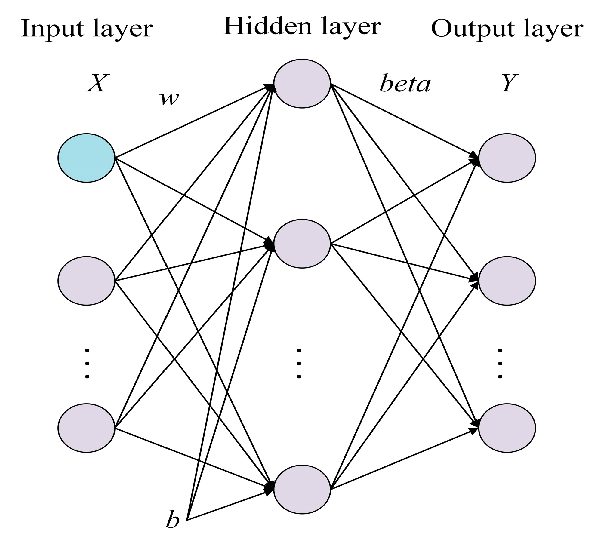
The extreme learning machine (ELM) overcomes shortcomings of slow learning speed and complicated steps of the BP neural network [25], and efficiency and generalization of machine learning are boosted [26]. In the ELM model with P input nodes, K hidden nodes and L output nodes as shown in Figure 2, Suppose that there are n data samples $\left(x_i,t_i\right)$, H is the output of hidden layer, β is the weight of the output layer, and T is the expected output. The ELM structure is shown in Equations (6)–(8):

$$H_{N\times K}=\left[\begin{array}{ccc}f\left(w_1·x_1+b_1\right)& \dots & f\left(w_K·x_1+b_K\right)\\ ⋮& ⋮& ⋮\\ f\left(w_1·x_N+b_1\right)& \dots & f\left(w_K·x_N+b_K\right)\end{array}\right]$$

(6)

$${\beta }_{K\times L}=\left[{\beta }_1,\dots ,{\beta }_K\right]$$

(7)

$$T_{N\times L}=\left[t_1,\dots ,t_N\right]$$

(8)

According to the least square principle, connection weight β is calculated as Equation (9):

$$\mathsf{\beta }={\mathrm{H}}^{+}T$$

(9)

where ${\mathrm{H}}^{+}$ is the Moore-Penrose general inverse matrix.

2.4. Improved Bat Algorithm

Bat algorithm (BA) is a kind of intelligent optimization algorithm established by simulating the echolocation behavior of bats. BA has the double advantage of global search and local search, which effectively improves the optimization processing ability of the problem [27]. However, BA lacks the mechanism of information exchange between individuals [28]. In this paper, the strategy of horizontal crossover is used to improve BA (IBA) to further enhance the optimization ability and speed of the BA algorithm. The basic steps are as follows:

(1)

Suppose that the instantaneous flight rate of the ith bat in position $x_i$ is $v_i$, the search frequency is $fr{e}_i$, and the pulse loudness and the pulse emissivity are $so{n}_i$ and $ra{d}_i$, respectively. Where, $fr{e}_i$ is in the range of $\left[fremi{n}_i,frema{x}_i\right]$.

(2)

Frequency, speed and location of bat is updated as Equations (10)–(12):

$$fr{e}_i=fremi{n}_i+\left(frema{x}_i-fremi{n}_i\right)\alpha$$

(10)

$$v_i^{t+1}=v_i^t+\left(x_i^t-x_g^t\right)fr{e}_i$$

(11)

$$x_i^{t+1}=x_i^t+v_i^{t+1}$$

(12)

where, α is a random value from 0 to 1, t is number of iterations, and $x_g^t$ is the current optimal solution.

(3)

The horizontal cross strategy is used to share the population information and update the current individual speed and location as Equations (13) and (14).

$$v_i^{t+1}=\left(x_i^t-x_j^t\right)fr{e}_i$$

(13)

$$x_{i*}^{t+1}=x_i^t·rand+x_j^t·\left(1-rand\right)+v_i^{t+1}$$

(14)

(4)

Whether bats walk randomly or not is determined according to a randomly generated number [29]. ξ is a random number in [0,1]. Equation (15) shows its way of walking:

$$x_{new}=x_{old}+\xi so{n}_i$$

(15)

(5)

The loudness and pulse rate vary with iteration as Equations (16) and (17):

$$so{n}_i^{t+1}=\omega ·so{n}_i^t$$

(16)

$$ra{d}_i^{t+1}=ra{d}_i^0\left(1-\exp \left(-\sigma t\right)\right)$$

(17)

where ω and σ are constants greater than 0.

(6)

Calculate the optimal solution of the current bat swarm and terminate the algorithm if the solution meets the requirements. Otherwise, go to step (2).

3. Data Preprocessing

3.1. Data Sources

Based on historical trading data of the European Climate Exchange (ECX) and Korea Exchange (KRX) carbon markets, this paper makes an empirical study of carbon price prediction. The transaction data from 28 November 2016 to 13 September 2019 is selected as the ECX data set, while the transaction data from 12 January 2015 to 9 August 2018 is selected as the KRX data set. Simultaneously, the last 130 days and 180 days transaction prices of the two data sets are used as test sets, respectively, while the rest are used as training sets.

Table 1. Carbon price raw data in ECX and KRX.

Market	Type	Size	Training Set	Test Set	Training Set Period	Test Set Period	Date
ECX	EUA	669	539	130	2016/11/28–2019/3/13	2019/3/14–2019/9/13	2016/11/28–2019/9/13
KRX	KAU	881	701	180	2015/1/12–2017/11/15	2017/11/16–2018/8/9	2015/1/12–2018/8/9

and

Table 2. Descriptive statistics of carbon price data.

Sample	Mean	SD	Minimum	Median	Maximum	Skewness
ECX	14.29	8.19	4.30	13.68	29.81	1.25
KRX	14.52	4.14	7.18	15.39	23.29	−1.28

describe the basic information and statistical characteristics of empirical analysis samples, respectively.

The two selected samples’ data have high volatility and long time periods, which is conducive to in-depth identification of carbon price fluctuations. The sample data contains carbon price data of different days in the same week, which is conducive to study week-end effect of carbon price. The training sample sizes of ECX and KRX are 539 and 701, respectively, which can effectively verify the influence of differentiated samples on the stability of carbon price prediction. Therefore, the selected carbon price samples are representative, verifying the stability and superiority of the proposed carbon price prediction model.

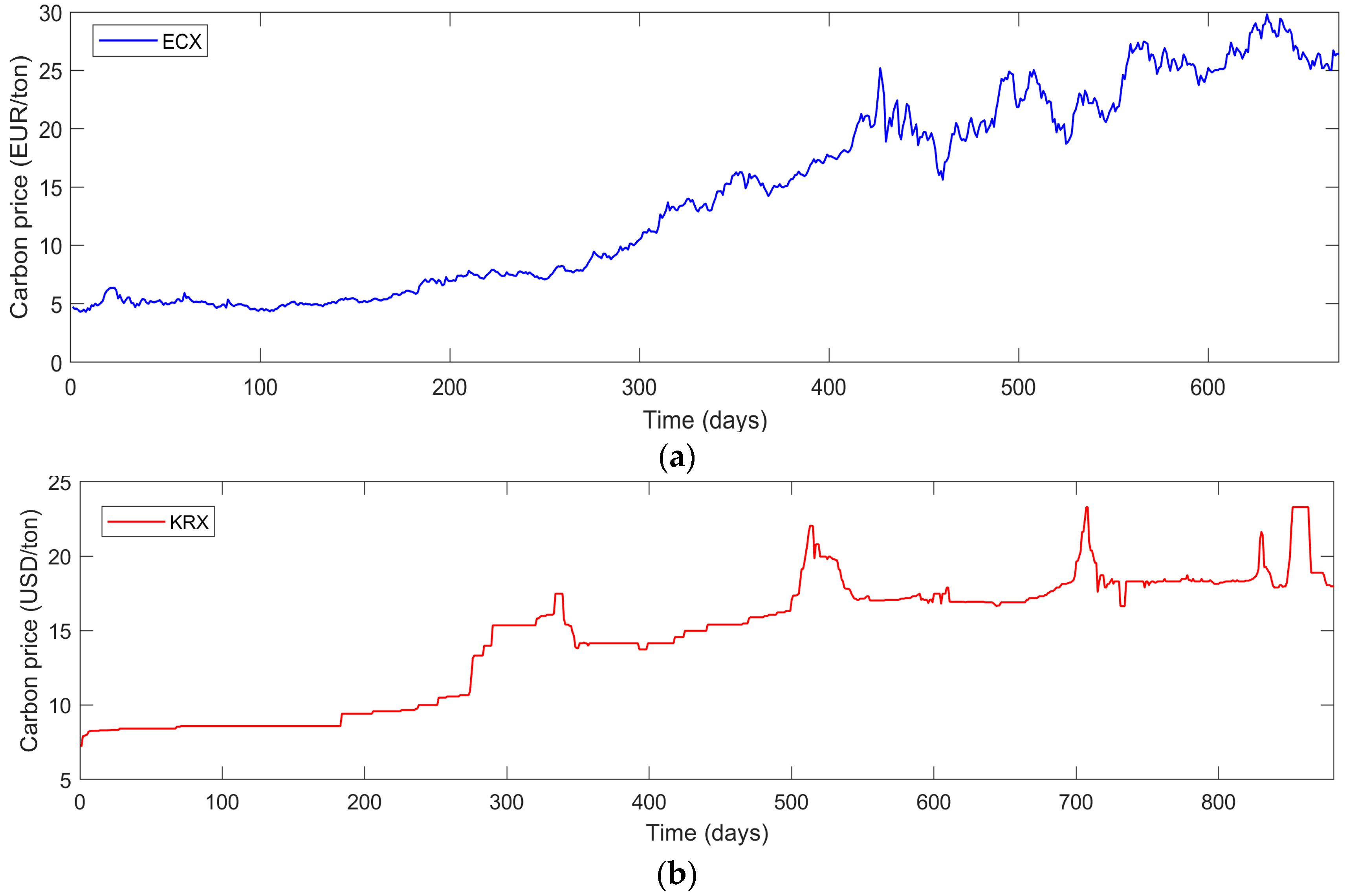
Take ECX and KRX carbon prices as empirical data to test the accuracy and stability of the EEMD-IBA-ELM model. Considering the currency unit universality, the carbon price of KRX is converted to international currency USD. The conversion relationship between KRW and USD is expressed as Equation (18), where, λ represents the exchange rate between KRW and USD in corresponding date of carbon price. The carbon price data of ECX and KRX are shown in Figure 3.

$$1 \mathrm{KRW}=\lambda \mathrm{USD}$$

(18)

In addition, the historical data of Brent crude oil futures price (BCOFP), New York Mercantile Exchange (NYMEX) natural futures price (NGFP), and West Texas Intermediate (WTI) crude oil future price (WTOFP) are used to reflect the fluctuation of energy prices in the world, so as to verify whether the introduction of energy price factors can improve carbon price prediction accuracy.

3.2. BDS Test and Carbon Price Structure Analysis

The BDS test is a classic time series nonlinear feature diagnosis method. It is the basis of carbon price research to analyze the internal law and dynamic structure of carbon price sequence. Therefore, the BDS method is used to test random walk fitting residuals of carbon prices in ECX and KRX [30]. In the BDS test, m represents dimension, n represents replication number, and W_{m, n} represents test statistics. Aiming to effectively identify the non-linear trend of carbon price, the autoregressive model (AR) model is first used to fit linear characteristics of carbon price. Secondly, carbon price residuals are calculated and standardized to form standard residuals. Original values, linear parts, and standard residuals of carbon prices in ECX and KRX are shown in Figure 4. Simultaneously, the BDS method is used to test standard residuals of carbon prices in the two markets and

Table 3. BDS test of carbon price.

Market	Dimension (m)	Test Statistics (Wm,n)
ECX	2	7.853
	3	9.274
	4	9.693
KRX	2	8.407
	3	9.102
	4	9.445

shows BDS test results. In Table 3, the values of test parameters W_{m, n} of carbon price in ECX and KRX are significantly not equal to zero, which indicates that there are obvious nonlinear characteristics and dynamic structure in carbon price series.

3.3. Weekend Effect Analysis

The weekend effect will affect carbon price volatility and characteristics, so carbon price weekend effect of ECX and KRX are tested in

Table 4. Weekend effect of carbon price.

Market	Statistic Indicators	Monday	Tuesday	Wednesday	Thursday	Friday
ECX	Mean	14.25	14.21	14.29	14.19	14.48
	SD	8.25	8.21	8.19	8.23	8.42
	Skewness	0.2527	0.2709	0.276	0.2816	0.3059
KRX	Mean	14.47	14.53	14.47	14.54	14.59
	SD	4.21	8.57	4.12	4.16	17.22
	Skewness	−0.2474	−0.3173	−0.3091	−0.3275	−0.3329

. The average carbon price of ECX and KRX on Fridays are significantly different from the other four weekdays. Meanwhile, the SD value of Friday’s carbon price was significantly higher than those of the other four weekdays. In particular, in the KRX carbon market, the value reached 17.22, which indicates that a weekend effect caused abnormal fluctuations in carbon prices. When the weekend approaches, carbon price skewness value shows an upward trend, which shows that the symmetry of carbon price is weakened by the weekend effect.

Considering day-of-the-week effect and weekend effect of carbon price data, day type of carbon price is quantified: {Monday, Tuesday, Wednesday, Thursday, Friday} = {1, 2, 3, 4, 5}. Simultaneously, the day type and carbon price value of the same weekday in the last three weeks are taken as input variables of EEMD-IBA-ELM to strength the prediction effect.

3.4. Carbon Price Decomposition

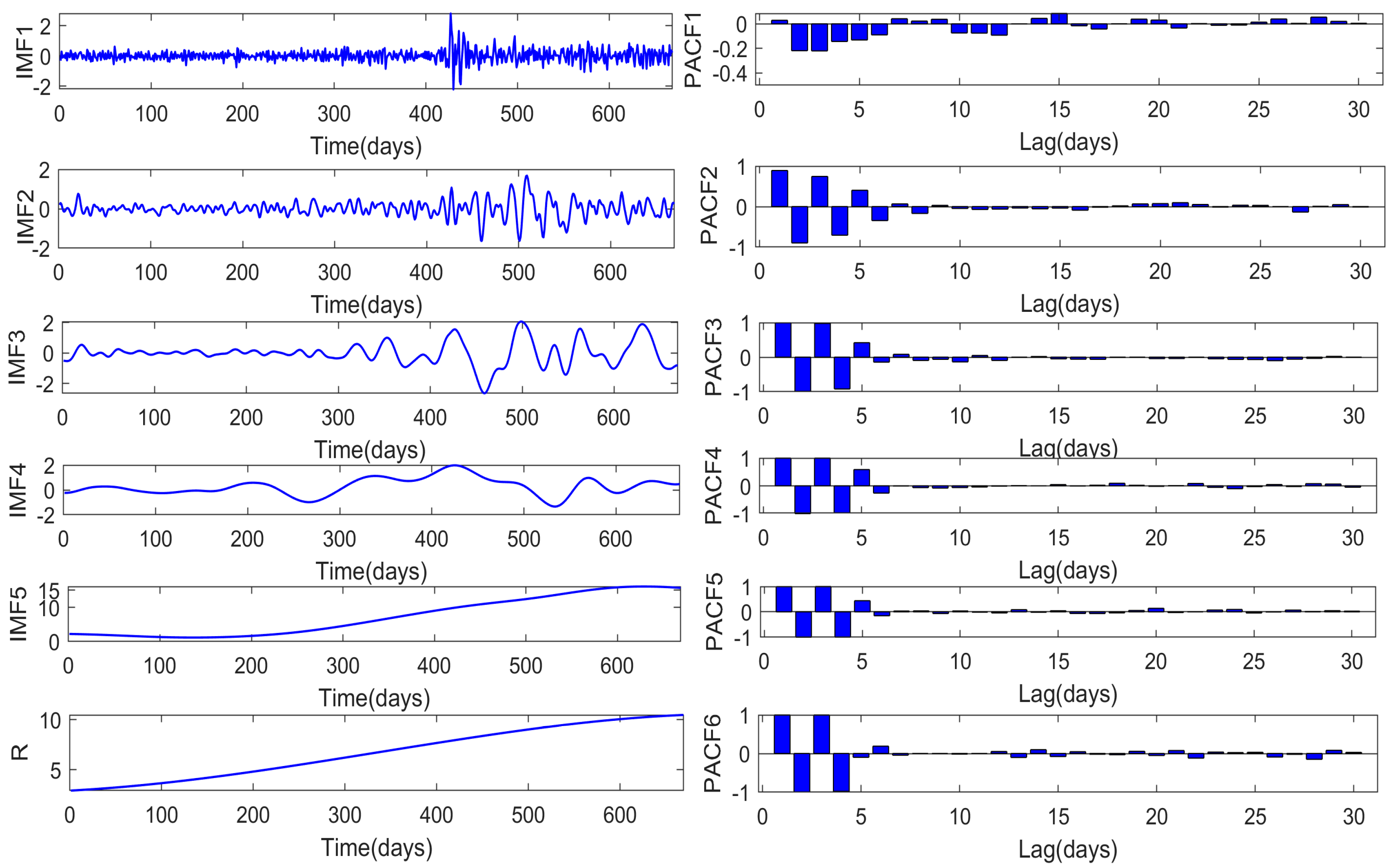
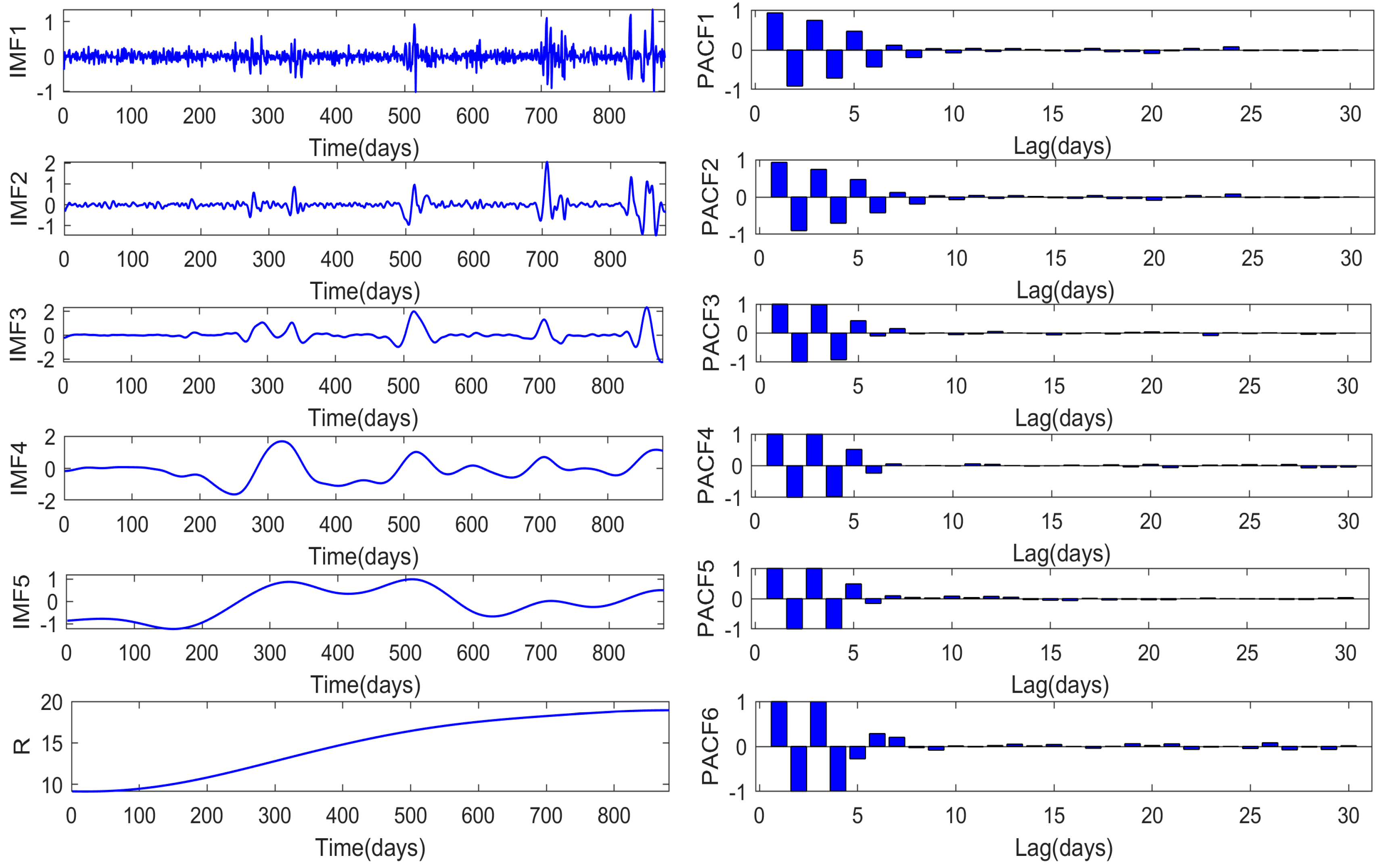
Aiming to separate carbon price series with higher accuracy and enhance the independence of each mode effectively to reduce information overlap, EEMD is used to realize carbon price decomposition of ECX and KRX. Evenly distributed white noise sequences with amplitude center of 0 are added to the original sequence many times, and each noise sequence is decomposed by EMD. Finally, multiple decomposition results of each mode are integrated into the final mode sequence according to the EEMD principle. Figure 5 and Figure 6 show the EEMD decomposition results of two carbon markets. It can be seen from the EEMD decomposition results of carbon price that the regularity of each IMF is more obvious than that of single EMD, which shows that noise-assisted EEMD is effective in carbon price decomposition.

In Figure 5 and Figure 6, the carbon price IMF components have obvious symmetry law, and the frequency of the obtained IMFs gradually decreases as the IMF’s serial number rises. In different time periods, the IMF has a regular frequency and amplitude range, which shows that EEMD effectively captures the law of carbon price and realizes modal decomposition.

By further checking the carbon price decomposition effect of EEMD, the description characteristics of EEMD components of two carbon markets in ECX and KRX are calculated; the results are shown in

Table 5. Descriptive statistics of carbon price EEMD and components in ECX and KRX.

Market	Components	Mean	SD	Mimimum	Median	Maximum	Skewness
ECX	IMF1	0.0038	0.3909	−2.2287	0.0001	2.8045	0.3790
	IMF2	−0.0011	0.4092	−1.6321	0.0004	1.6827	−0.2060
	IMF3	−0.0269	0.5749	−2.6533	−0.0361	2.0541	0.0029
	IMF4	0.2866	0.4747	−1.3384	0.2588	1.9815	0.1118
	IMF5	7.3055	5.5195	1.1721	6.0768	16.0863	0.3380
	R	6.7208	6.0117	2.9243	6.7214	10.4722	−0.0036
KRX	IMF1	0.0011	0.2071	−1.0185	−0.0005	1.3511	0.6258
	IMF2	−0.0079	0.3104	−1.4656	0.0003	2.0611	0.8786
	IMF3	0.0380	0.5236	−2.2590	−0.0017	2.3402	0.7472
	IMF4	−0.1076	0.6840	−1.6152	−0.0910	1.6810	0.3660
	IMF5	−0.0794	0.6588	−1.2331	−0.0640	0.9932	−0.1007
	R	14.6785	3.4874	9.1360	15.5251	18.9272	−0.3352

. When comparing the standard deviation (SD) of the two markets carbon prices before and after EEMD decomposition, the SD of the decomposed data is smaller than that of the original data. The results show that EEMD significantly reduces the dispersion and irregularity of carbon price. Simultaneously, by comparing the skewness of carbon price before and after EEMD decomposition, it can be found that the skewness of EEMD components is lower than that of the original data, except for the residual component R. This shows that the IMFs obtained from EEMD decomposition have significant symmetry characteristics, when compared to the original carbon price. In addition, R has no obvious symmetry because it represents the main trend of carbon price change. Therefore, EEMD can effectively identify the internal law of carbon price and improve the decomposition effect.

3.5. Selection of Factors Influencing Carbon Price

From autocorrelation of carbon price and influence of energy price, we search for influencing factors of carbon price and determine input variables of the EEMD-IBA-ELM carbon price model. In terms of historical carbon price, PACF is applied to measure correlation between current carbon price and historical carbon price. Simultaneously, the autocorrelation factors of carbon price were determined according to PACF analysis. The autocorrelation influence variables of EEMD decomposition components in the ECX and KRX carbon markets are shown in

Table 6. PACF analysis of carbon price after EEMD.

Component	Lag
	ECX	KRX
IMF1	2, 3	1, 2,3, 4, 5, 6
IMF2	1, 2, 3, 4, 5, 6	1, 2, 3, 4,5, 6
IMF3	1, 2, 3, 4, 5	1, 2, 3, 4, 5
IMF4	1, 2, 3, 4	1, 2, 3, 4,5
IMF5	1, 2, 3, 4	1, 2, 3, 4, 5
R	1, 2, 3, 4	1, 2, 3, 4

, Figure 5, and Figure 6.

Table 7. Partial autocorrelation analysis coefficient of carbon price EEMD components in ECX.

Lag	Partial Autocorrelation Coefficient
	IMF1	IMF2	IMF3	IMF4	IMF5	R
1	0.0292	0.8931	0.9930	0.9986	0.9969	0.9987
2	−0.2184	−0.8968	−0.9900	−0.9978	−0.9985	−0.9980
3	−0.2202	0.7453	0.9782	0.9988	0.9928	0.9986
4	−0.1433	−0.7060	−0.9201	−0.9687	−0.9693	−0.9781
5	−0.1313	0.4044	0.4192	0.5867	0.4405	−0.0986
6	−0.0895	−0.3435	−0.1442	−0.2579	−0.1545	0.1900

shows partial correlation coefficients of ECX carbon price IMFs.

According to PACF analysis in Figure 5 and Figure 6, we can find that carbon price IMFs are mainly affected by the first several lag variables. When the lag period is greater than 6, correlation between lag variable and IMF decreases significantly. Therefore, the sixth lag variable can be used as an interface of IMF autocorrelation factors. In Table 7, the autocorrelation factors of IMF are selected from the first six lag variables, according a PACF coefficient.

In Figure 5, there is a strong autocorrelation between the IMF1 of ECX carbon price and its second and third lagged variables, and there is a significant negative correlation between the two influencing factors and carbon price. From the fourth lag variable, there is only a weak correlation between the lag variable and carbon price. Therefore, the second and third lagged variables can be taken as the influencing factors of IMF1 of ECX carbon price. In the same way, the remaining IMFs and R of ECX carbon price are strongly correlated with the previous lagged variables, and there is a clear boundary between the strongly correlated lagged variables and the weakly correlated lagged variables. In Figure 6, a similar conclusion can be drawn from the PACF analysis of KRX carbon market. Therefore, by extracting the influencing factors of carbon price IMFs and R according to partial correlation coefficient, the main internal influencing factors of carbon price are included in a few selected variables, which reduces the number of input variables of carbon price prediction model and increases representativeness of the influencing factors of carbon price.

BCOFP, NGFP, and WTOFP reflect price fluctuation of world major energy futures. BCOFP and WTOFP represent the fluctuation of international oil price, while NGFP represents natural gas price information. Changes in energy prices influence the relationship between energy supply and demand and lead to changes in carbon emissions, which promotes the fluctuation of carbon demand and price.

In addition, person correlation coefficients of BCOFP, NGFP, and WTOFP with ECX carbon price were 0.742, 0.598, and 0.748, respectively. The person correlation coefficients of BCOFP, NGFP, and WTOFP with KRX carbon price were 0.729, 0.522, and 0.865, respectively. The results show that there is evident correlation between the three selected variables reflecting energy prices and carbon prices. Therefore, BCOFP, NGFP, and WTOFP are used as input variables of the EEMD-IBA-ELM carbon price model to enhance information capture ability of the model and improve prediction effect.

4. Empirical Analysis of Carbon Price Prediction

Aiming to test accuracy and stability of the carbon price model, ECX and KRX carbon trading prices were selected as data samples. These two carbon markets have significant differences in trading volume and carbon price volatility, which can effectively test the prediction effect of the carbon price model on differentiated carbon price and universality of the model. Simultaneously, the classic BP and SVM intelligent prediction methods are used as comparison methods in this part to verify superiority of the EEMD-IBA-ELM carbon price model.

4.1. Parameter Setting

Compared to the traditional neural network, single ELM has a higher learning speed and better optimization strategy, but the model lacks stability and depth optimization ability. The weight and threshold parameters generated randomly cannot ensure that ELM can build superior intelligent structure every time. Here, sigmoid is used to realize the kernal mapping of ELM. Combining ELM with the improved BA algorithm, the IBA-ELM carbon price prediction model is established.

The number of hidden layers is the basic parameter of ELM. For different data types and practical problems, the number of hidden layers of elm should be set according to specific needs. Too few hidden layers make it difficult to extract the effective information of input variables, and a large number of useful information is over compressed. Simultaneously, too many hidden layers will lead to over fitting of ELM, and the effect of a large number of invalid information will be magnified, resulting in nonideal final model output. Referring to the number of input variables of the IBA-ELM carbon price model, the hidden layer node of ELM is set to 9.

In bat algorithm, pulse loudness and emissivity affect the speed and accuracy of individual bat optimization. The number of bat individuals and iterations should be large enough. Too few bats impact the stability of the algorithm, and cannot produce ideal output results in some optimization processes. Simultaneously, lack of iterations will also lead to the current global optimal solution not meeting the set requirements. In addition, sufficient bat individuals are the basis and condition for the realization of information interaction mechanism, and also guarantee the effectiveness of the IBA algorithm. Combined with the effective IBA algorithm and ELM, IBA-ELM will produce stable prediction results.

4.2. Training Carbon Price Model

Aiming to optimize the IBA-ELM algorithm and build a robust IBA-ELM carbon price model, the influencing factors of carbon price are taken as the eigenvalues of bats in the IBA algorithm, and ELM prediction error is taken as a fitness function value of the IBA algorithm. Figure 7a,b shows parameter space and iterative curve of the IBA algorithm, respectively. In Figure 7a, weight w, threshold b, and fitness of ELM constitute parameter space of ELM. A global optimal fitness value is seen. Single ELM has randomness of parameters and it is difficult to find the parameters w and b corresponding to the optimal fitness effectively. Therefore, IBA is used to quickly find the optimal values of ELM parameters w and b and Figure 7b shows the search process of IBA. The iteration curve of IBA shows that the error of IBA-ELM decreases gradually with increase in calculation times and tends to be stable after the 25th iteration, indicating that the model has found a better solution. Although the solution is not necessarily the optimal solution, the error of the solution is infinitely close to the global optimal solution and meets the needs of carbon price prediction.

4.3. Carbon Price Prediction and Error Evaluation

As the selection of parameters affects the convergence effect of BA and stability of ELM, the basic parameters of BA and ELM are selected as shown in

Table 8. Model parameter setting.

Model	Parameters	Value
IBA	Maximum pulse	3
	Minimum pulse	0
	Number of bat	50
	Maximum loudness	0.8
	Initial pulse emissivity	0.12
	Maximum number of iterations	50
ELM	Hidden layer node	9
	Kernel function	sig

. The EEMD-IBA-ELM prediction model is set with the parameters in Table 8, and the carbon prices of ECX and KRX are empirically predicted. Simultaneously, mean absolute error (MAE), root mean square error (RMSE), and mean absolute percent error (MAPE) are used to measure prediction effect as Equations (19)–(21) when P_MAE, P_RMSE and P_MAPE are used to measure improvement degree as Equations (22)–(24):

$$\mathrm{MAE}=\frac{1}{n}{{\displaystyle \sum }}_{i=1}^n\left|{\widehat{y}}_i-y_i\right|$$

(19)

$$\mathrm{RMSE}=\sqrt{\frac{1}{n}{{\displaystyle \sum }}_{i=1}^n{\left({\widehat{y}}_i-y_i\right)}^2}$$

(20)

$$\mathrm{MAPE}=\frac{1}{n}{{\displaystyle \sum }}_{i=1}^n\left|\frac{{\widehat{y}}_i-y_i}{y_i}\right|\times 100\%$$

(21)

$${\mathrm{P}}_{\mathrm{MAE}}=\frac{{\mathrm{MAE}}_{\mathrm{a}}-{\mathrm{MAE}}_{\mathrm{b}}}{{\mathrm{MAE}}_{\mathrm{a}}}\times 100\%$$

(22)

$${\mathrm{P}}_{\mathrm{RMSE}}=\frac{{\mathrm{RMSE}}_{\mathrm{a}}-{\mathrm{RMSE}}_{\mathrm{b}}}{{\mathrm{RMSE}}_{\mathrm{a}}}\times 100\%$$

(23)

$${\mathrm{P}}_{\mathrm{MAPE}}=\frac{{\mathrm{MAPE}}_{\mathrm{a}}-{\mathrm{MAPE}}_{\mathrm{b}}}{{\mathrm{MAPE}}_{\mathrm{a}}}\times 100\%$$

(24)

where, ${\widehat{y}}_i$ and $y_i$ represents predicted value and actual value, respectively. Simultaneously, a represents the basic model and b represents the optimization model.

5. Results and Discussion

5.1. Comparing Prediction Results with the Random Walk Model

Comparative analysis of prediction accuracy is an important evaluation requirement of carbon price prediction. In statistical significance, the EEMD-IBA-ELM model and the simple random walk model are compared by the Morgan-Granger-Newbold test [31]. Considering EEMD-IBA-ELM and simple random walk forecasts, the test statistics are MGN are 5.5864 and 9.0233 in ECX and KRX carbon markets, respectively, which shows that the EEMD-IBA-ELM model has more advantages than the simple random walk model in carbon price forecast.

5.2. Comparing Prediction Results with Statistical Models

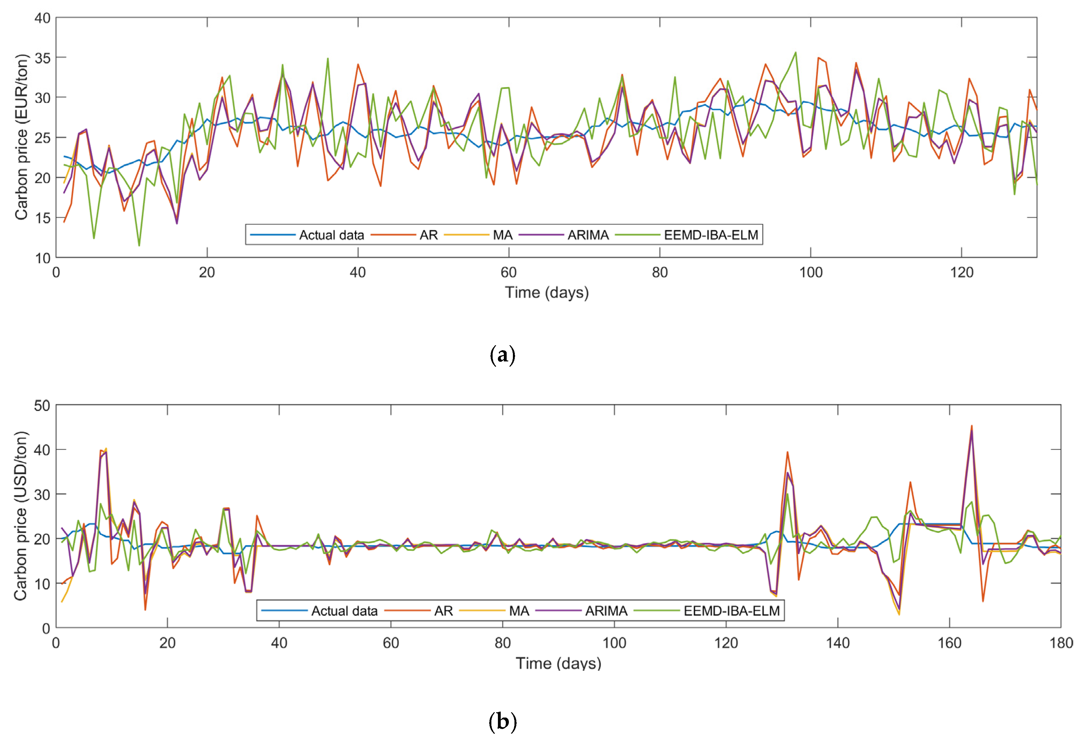
Aiming to further test the prediction effect of EEMD-IBA-ELM compared to statistical carbon price models, AR (autoregressive model), MA (moving average model), and ARIMA (autoregressive integrated moving average model) were used as control models to predict carbon price. The comparison results are shown in Figure 8 and

Table 9. Comparative analysis with statistical models.

Carbon Market	ECX			KRX
Error Criterion	MAE	RMSE	MAPE	MAE	RMSE	MAPE
AR	3.8494	6.2418	19.8412	3.7069	7.0727	19.1063
MA	3.5857	6.0285	18.3189	3.4529	6.8310	17.6404
ARIMA	3.3460	5.7139	17.1816	3.2220	6.4745	16.5452
EEMD-IBA-ELM	2.9063	3.6968	11.2652	2.7121	3.5120	10.1353

. It can be seen from Figure 8 that the EEMD-IBA-ELM model can predict a fluctuation trend of carbon price more effectively than AR, MA, and ARIMA models. Simultaneously, in Figure 8b, there is a big deviation between the predicted results of the AR model and the actual carbon price in some range. One possible reason is that the statistical model has poor nonlinear fitting ability and it is difficult to extract the nonlinear characteristics of the data effectively. From the error analysis results of Table 9, the prediction error of the two carbon markets of EEMD-IBA-ELM is significantly lower than that of the comparative statistical model, which shows superiority of the proposed model.

5.3. Comparing Prediction Results with Combined Models

Based on the MATLAB (produced by MathWorks, Natick, Massachusetts, USA) data analysis platform, EEMD-IBA-ELM is used to predict the carbon price of ECX and KRX. The validity and stability of the EEMD-IBA-ELM model were tested by comparing the prediction effect of the EEMD-IBA-ELM model with contrast models. Figure 9 shows the model comparison framework. The green part represents the decomposition method of carbon price and external input variables of carbon price, the blue part represents the basic carbon price prediction and optimization models, and the yellow part represents 11 carbon price comparison models.

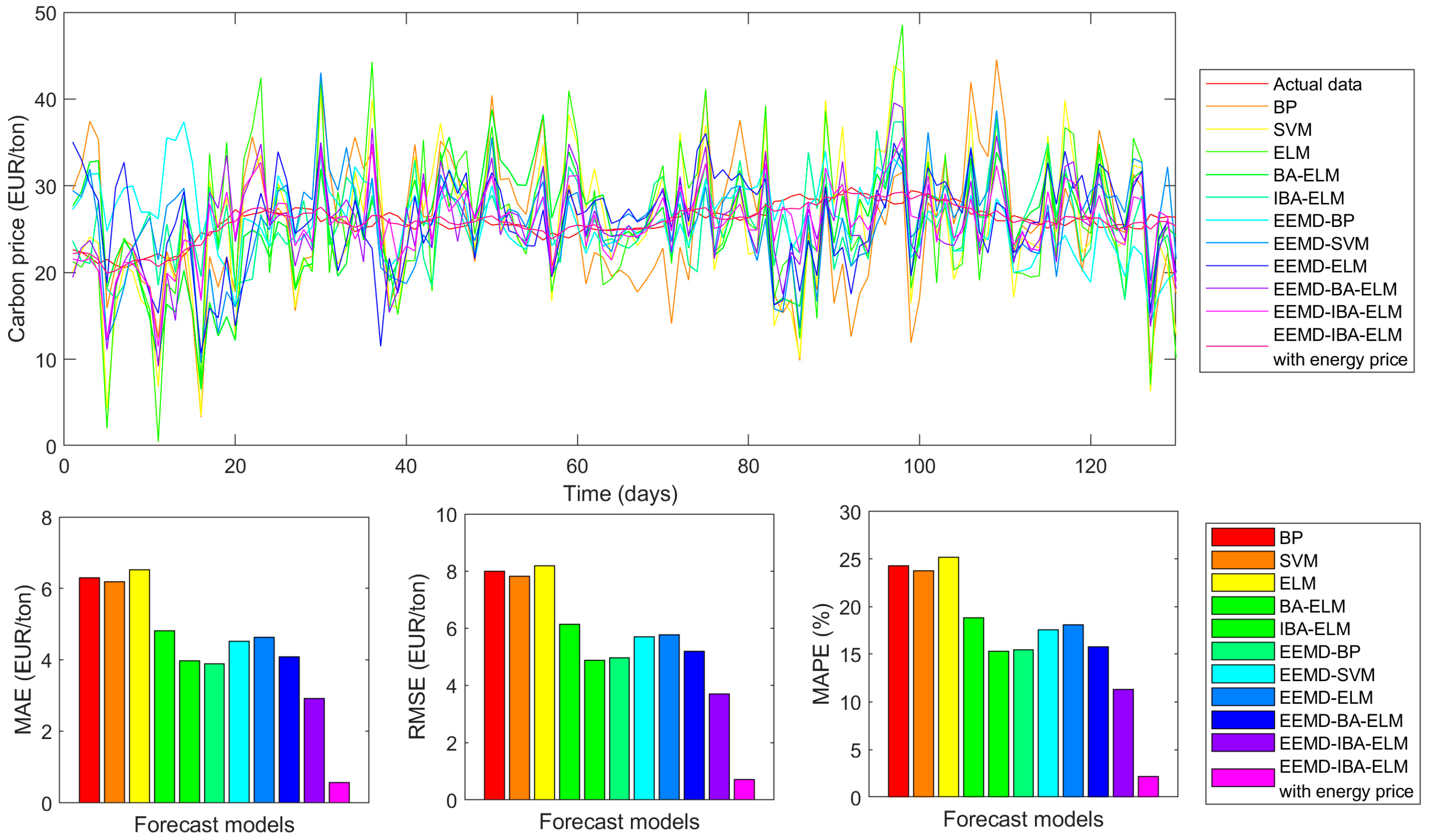
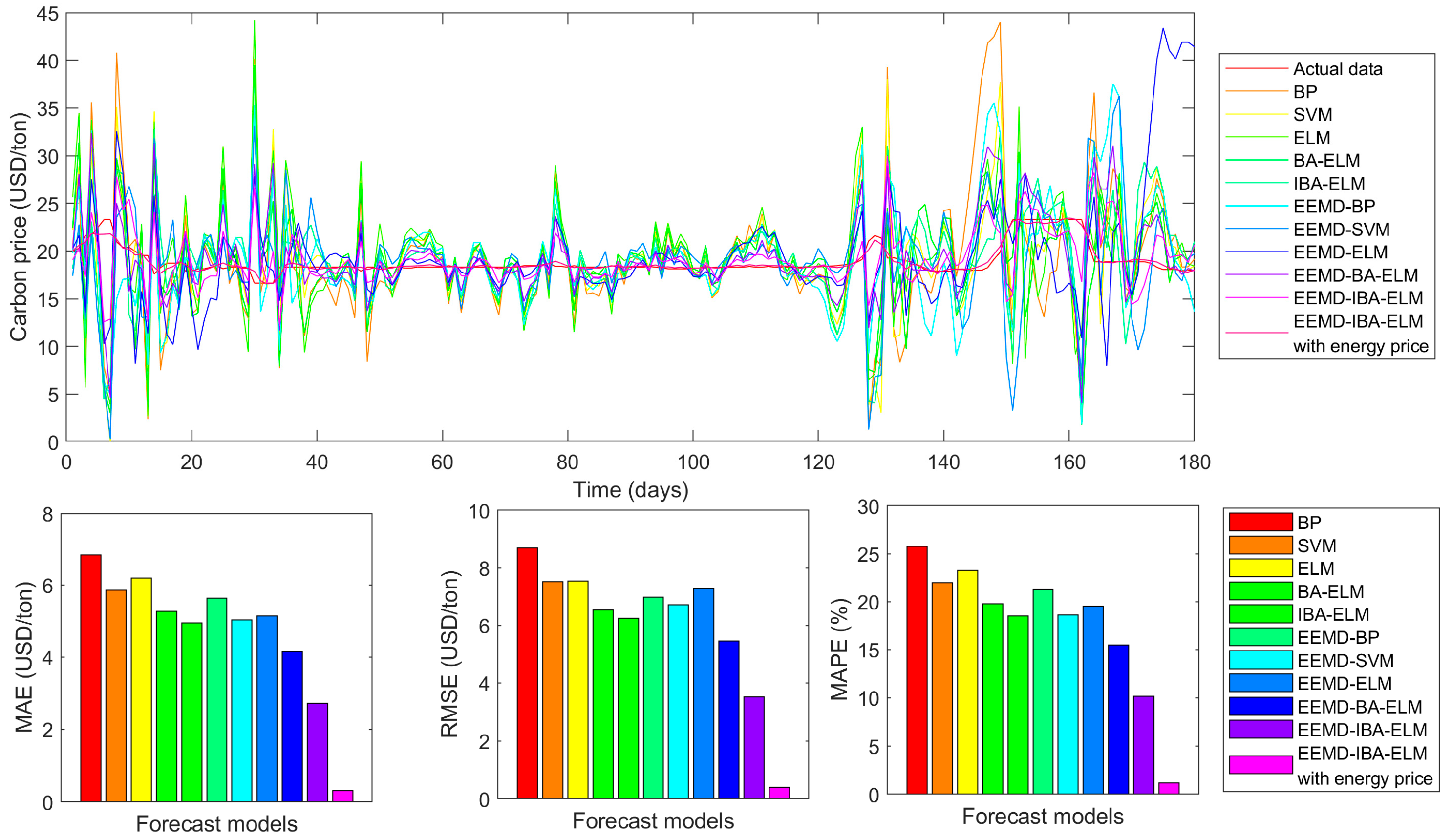
Figure 10 and Figure 11 show the carbon price prediction results of ECX and KRX, respectively, when the error analysis value is shown in

Table 10. Error analysis of carbon price prediction.

Carbon Market	ECX			KRX
Error Criterion	MAE	RMSE	MAPE	MAE	RMSE	MAPE
BP	6.3006	7.9828	24.3050	6.8907	8.7945	25.8796
SVM	6.1787	7.8241	23.7845	5.9481	7.7521	22.2130
ELM	6.5217	8.1874	25.1835	6.5123	8.4018	24.2136
BA-ELM	4.8095	6.1307	18.8201	5.3906	6.8655	20.1185
IBA-ELM	3.9606	4.8659	15.2662	4.9443	6.2430	18.5033
EEMD-BP	3.8745	4.9609	15.4382	5.7753	7.4442	21.6634
EEMD-SVM	4.5172	5.6911	17.5597	5.0558	6.7947	18.6797
EEMD-ELM	4.6314	5.7632	18.0786	5.1434	7.2756	19.4996
EEMD-BA-ELM	4.0839	5.1819	15.7496	4.1419	5.4532	15.4697
EEMD-IBA-ELM	2.9063	3.6968	11.2652	2.7121	3.5120	10.1353
EEMD-IBA-ELM with energy price	0.5688	0.7047	2.1982	0.3145	0.4024	1.1762

.

The improvement effect of carbon price prediction is shown in Figure 12 and

Table 11. Model comparison and improvement effect analysis.

Market	Contrast Model		Improved Model	PMAE	PRMSE	PMAPE
ECX	BP	vs.	EEMD-BP	38.5061	37.8547	36.4814
	SVM	vs.	EEMD-SVM	26.8898	27.2627	26.1714
	ELM	vs.	EEMD-ELM	28.9846	29.6086	28.2127
	EEMD-ELM	vs.	EEMD-BA-ELM	11.8213	10.0869	12.8826
	EEMD-BA-ELM	vs.	EEMD-IBA-ELM	28.8361	28.6595	28.4728
	EEMD-IBA-ELM	vs.	EEMD-IBA-ELM with energy price	80.4297	80.9388	80.4865
KRX	BP	vs.	EEMD-BP	16.1876	15.3538	16.2915
	SVM	vs.	EEMD-SVM	15.0013	12.3506	15.9062
	ELM	vs.	EEMD-ELM	21.0197	13.4037	19.4683
	EEMD-ELM	vs.	EEMD-BA-ELM	19.4719	25.0484	20.6670
	EEMD-BA-ELM	vs.	EEMD-IBA-ELM	34.5200	35.5975	34.4829
	EEMD-IBA-ELM	vs.	EEMD-IBA-ELM with energy price	88.4026	88.5430	88.3951

.

Based on the above results, the following conclusions can be drawn:

(1)

By analyzing the trend chart of two carbon market prediction results, the single BP, SVM, and ELM models have a larger deviation range in carbon price predictions than the actual carbon prices, while the single model has a poor fitting effect on the carbon price trend. Simultaneously, in the prediction experiment of ECX carbon market, the prediction value of single SVM and ELM model is mostly smaller than the actual value. The error distribution of the prediction result is not symmetrical, which brings difficulties to carbon price prediction and research. Therefore, it is necessary to improve and optimize the single ELM carbon price model. The prediction effect of ELM optimized by IBA on carbon price trend is obviously improved.

(2)

When comparing the prediction error values of BP, SVM, and ELM in ECX and KRX carbon markets, the MAE, RMSE, and MAPE of SVM are the minimum values (6.1787%, 7.8241%, and 23.7845% in ECX; 5.9481%, 7.7521% and 22.2130% in KRX). Because of the instability and parameter randomness, single ELM is not effective in the prediction experiments in ECX and KRX. However, BA-ELM’s three forecast errors dropped to 4.8095%, 6.1307%, and 18.8201% in the ECX market, while BA-ELM’s three forecast errors dropped to 5.3906%, 6.8655%, and 20.1185% in the KRX market. When BA with information interaction mechanism is used to optimize ELM, IBA-ELM’s three forecast errors dropped to 3.9606%, 4.8659%, and 15.2662% in the ECX market, and BA-ELM’s three forecast errors dropped to 4.9443%, 6.2430%, and 18.5033% in the KRX market, which shows that information interaction mechanism significantly enhances the cooperation of bat individuals in BA and improves the efficiency of carbon price model parameters optimization.

(3)

Comparing the prediction models, including the decomposition of carbon price with those without data processing, it was found that prediction errors of EEMD-BP, EEMD-SVM, and EEMD-ELM are lower than those of the corresponding single prediction model, which shows that decomposition of carbon price by EEMD can reduce difficulty of carbon price prediction and enhance the prediction effect. Simultaneously, in the study of the KRX carbon market, RMSE of EEMD-ELM is slightly lower than that of EEMD-BP when MAE and MAPE of EEMD-ELM are higher than that of EEMD-SVM. These phenomena are caused by the single ELM model with poor stability. When IBA is used to improve ELM and EEMD-IBA-ELM is constructed, the prediction error is significantly improved, when compared to EEMD-BP, EEMD-SVM, and EEMD-ELM.

(4)

When BCOFP, NGFP, and WTOFP were introduced into the EEMD-IBA-ELM model as input variables, MAE, RMSE, and MAPE of EEMD-IBA-ELM decreased from 2.9063%, 3.6968%, and 11.2652% to 0.5688, 0.7047, and 2.1982%, respectively, in the ECX carbon market; MAE, RMSE, and MAPE of EEMD-IBA-ELM decreased from 2.7121%, 3.5120%, and 10.1353% to 0.3145%, 0.4024%, and 1.1762% in the KRX carbon market. BCOFP, NGFP, and WTOFP have proved to be useful for carbon management and can improve prediction ability and accuracy of carbon price.

(5)

By analyzing the improvement effect of EEMD on carbon price prediction, the improvement of EEMD to three single models is over 25% in the ECX carbon market. The P_MAE, P_RMSE and P_MAPE of EEMD-BP, EEMD-SVM, and EEMD-ELM are all over 25% and some indexes are over 40%, which shows that EEMD has an outstanding improvement effect in improving carbon price prediction ability. In prediction of KRX’s carbon market, EEMD improved three single models more than 10%. The improvement effect of EEMD in KRX carbon prediction is not as good as that in ECX carbon market because the volatility and amplitude of KRX carbon price are large, which reduces the space for improvement of carbon price prediction to some degree. Therefore, the use of EEMD can significantly reduce the complexity of carbon price data and improve prediction accuracy.

(6)

By analyzing the influence of BA optimization algorithm and energy price factors on carbon price prediction, the improvement degree of BA to EEMD-ELM is less than 15%, and the improvement degree of IBA to EEMD-BA-ELM is more than 28% in the ECX carbon market. In KRX’s carbon market, BA’s improvement on EEMD-ELM is nearly 20% and IBA’s improvement on EEMD-BA-ELM is nearly 35%. The difference between the experimental results of the two carbon markets is due to the difference of data and the improvement effect of EEMD. EEMD has a lower improvement effect on carbon prediction in KRX and IBA has a higher improvement effect, which shows that it is necessary to use EEMD and IBA together in the ELM carbon price model. In addition, after introducing energy price into the EEMD-BA-ELM carbon price model, the improvement degree of carbon market forecast in ECX is slightly higher than 80%, while that in KRX is higher than 88%. This shows that the help of energy price to carbon price prediction cannot be ignored. The EEMD-BA-ELM carbon price model combined with EEMD, IBA, and energy factors is effective.

5.4. Residual Test

In

Table 12. DW test of prediction residuals.

Carbon Market	ECX	KRX
BP	1.139	0.614
SVM	1.242	1.181
ELM	0.943	1.189
BA-ELM	1.220	1.273
IBA-ELM	1.413	1.333
EEMD-BP	1.204	1.219
EEMD-SVM	1.436	1.207
EEMD-ELM	1.157	1.429
EEMD-BA-ELM	1.746	1.528
EEMD-IBA-ELM	1.904	1.788
EEMD-IBA-ELM with energy price	1.943	1.930

, the Durbin Watson (DW) test is used to check possible autocorrelation in carbon price prediction residuals [32]. Carbon price forecast residuals of single BP, SVM, and ELM models have a positive correlation, which indicates that the single model has poor stability again. When EEMD is used to decompose and reconstruct carbon price, correlation of the predicted residuals is suppressed. Simultaneously, correlation of EEMD-IBA-ELM forecast residuals is very small, which shows that IBA significantly enhances stability and effectiveness of prediction. When considering energy price, correlation of EEMD-IBA-ELM’s prediction residual basically disappears, which shows that EEMD-IBA-ELM has superior prediction performance.

Overall, the main research results of the two carbon markets are as follows:

(1)

Using the data decomposed by EEMD improves the prediction accuracy of carbon price when prediction error of the single BP, SVM, and ELM model is large, which shows that EEMD can realize the accurate separation of independent modal components by adding white noise sequence to the original carbon price sequence.

(2)

Prediction accuracy of the BA-ELM composite model is higher than that of the single BP, SVM, and ELM model, whether original carbon price is decomposed by EEMD or not. Because the connection parameters between input layer and hidden layer are randomly set, prediction results of a single ELM model are very unstable, which leads to a large prediction error of single ELM. When ELM is optimized by BA, the prediction accuracy is improved and the model stability is enhanced. Simultaneously, because IBA further improves the optimization ability of the algorithm by using horizontal crossover strategy to optimize BA, the prediction accuracy of EEMD-IBA-ELM outperforms EEMD-BA-ELM. The prediction errors of EEMD-IBA-ELM in ECX and KRX carbon markets are 11.2652% and 10.1353%, respectively.

(3)

When BCOFP, NGFP, and WTOFP are used as input variables of EEMD-IBA-ELM, the prediction performance of EEMD-IBA-ELM is further enhanced. The prediction accuracy of EEMD-IBA-ELM considering energy price in the ECX and KRX markets was increased to 2.1982% and 1.1762%. BCOFP and NGFP are the main energy futures prices in the world. Their fluctuations affect energy supply, energy consumption structure, and international trade, thus further affecting price fluctuations in the carbon market. Furthermore, WTOFP reflects the change of supply and demand in the energy market, thus affecting carbon price fluctuation. The results show that introduction of BCOFP, NGFP, and WTOFP can significantly enhance carbon price prediction accuracy.

6. Conclusions

A novel carbon price prediction method is constructed based on EEMD, IBA, and ELM in this paper. First, EEMD improves the separation efficiency of carbon price components and high-precision carbon price characteristic IMFs are acquired. Secondly, IBA establishes the information sharing mechanism of the BA algorithm and improves its optimization efficiency by using horizontal cross strategy. Simultaneously, ELM is optimized by IBA to enhance the stability and prediction accuracy of the model. Finally, EEMD-IBA-ELLM is proven to be effective in carbon price prediction by comparing with the comparison model, and the introduction of BCOFP, NGFP, and WTOFP can further improve the prediction effect. The main conclusions of this study are as follows:

(1)

The carbon price sequence has significant complexity and irregularity. With the aid of white noise decomposition, the carbon price is decomposed into several independent feature components, which greatly reduces the difficulty of carbon price prediction and improves the prediction accuracy.

(2)

In the empirical analysis of the ECX and KRX carbon markets, EEMD-IBA-ELM has the best prediction accuracy and effect. Therefore, EEMD-IBA-ELM is an effective and feasible carbon price forecasting tool, which will help carbon market managers to supervise market operation and help carbon trading investors make investment decisions. At present, carbon markets are becoming more and more active and ECX and KRX carbon markets are typical representatives of the active carbon market. Therefore, EEMD-IBA-ELM is an effective method to predict current price fluctuation of carbon trading.

(3)

There is a high correlation between energy prices and carbon prices, which reflects that changes in energy systems have a significant impact on carbon emissions and carbon trading. By introducing the energy price factor into the EEMD-IBA-ELM carbon price model, we can achieve a more accurate prediction. In addition, the energy sectors can effectively reduce carbon emissions and promote development of the carbon market by adjusting energy supply and consumption structure.

In this study, a new method of carbon price analysis and prediction is established, which improves accuracy of carbon price prediction. Simultaneously, introduction of energy price can improve the prediction effect of carbon price. However, energy spot price is not considered due to lack of historical data. In the future, energy spot price can be considered in carbon price prediction.

References

1. Rabe, M.; Streimikiene, D.; Bilan, Y. EU carbon emissions market development and its impact on penetration of renewables in the power sector. Energies 2019, 12, 2961. [Google Scholar] [CrossRef] [Green Version]
2. Zhao, X.; Jiang, G.; Nie, D.; Chen, H. How to improve the market efficiency of carbon trading: A perspective of China. Renew. Sust. Energ. Rev. 2016, 59, 1229–1245. [Google Scholar] [CrossRef]
3. Lu, H.; Ma, X.; Huang, K.; Azimi, M. Carbon trading volume and price forecasting in China using multiple machine learning models. J. Clean. Prod. 2020, 249, 119386. [Google Scholar] [CrossRef]
4. Tian, C.; Hao, Y. Point and interval forecasting for carbon price based on an improved analysis-forecast system. Appl. Math. Model. 2020, 79, 126–144. [Google Scholar] [CrossRef]
5. Liu, H.; Shen, L. Forecasting carbon price using empirical wavelet transform and gated recurrent unit neural network. Carbon Manag. 2020, 11, 25–37. [Google Scholar] [CrossRef]
6. Sun, W.; Huang, C. A carbon price prediction model based on secondary decomposition algorithm and optimized back propagation neural network. J. Clean. Prod. 2020, 243, 118671. [Google Scholar] [CrossRef]
7. Zhu, B. A novel multiscale ensemble carbon price prediction model integrating empirical mode decomposition, genetic algorithm and artificial neural network. Energies 2012, 5, 355–370. [Google Scholar] [CrossRef]
8. Xiong, S.; Wang, C.; Fang, Z.; Ma, D. Multi-step-ahead carbon price forecasting based on variational mode decomposition and fast multi-output relevance vector regression optimized by the multi-objective whale optimization algorithm. Energies 2019, 12, 147. [Google Scholar] [CrossRef] [Green Version]
9. Sun, W.; Zhang, C.; Sun, C. Carbon pricing prediction based on wavelet transform and K-ELM optimized by bat optimization algorithm in China ETS: The case of Shanghai and Hubei carbon markets. Carbon Manag. 2018, 9, 605–617. [Google Scholar] [CrossRef]
10. Amanollahi, J.; Ausati, S. PM2.5 concentration forecasting using ANFIS, EEMD-GRNN, MLP, and MLR models: A case study of Tehran, Iran. Air. Qual. Atmos. Health 2020, 13, 161–171. [Google Scholar] [CrossRef]
11. Lin, S.N.; Lin, G.; Tsai, P.; Hsu, A.; Lo, M.; Yang, A.C.; Lin, C.; Wu, C.W. Sensitivity enhancement of task-evoked fMRI using ensemble empirical mode decomposition. J. Neurosci. Meth. 2016, 258, 56–66. [Google Scholar] [CrossRef] [PubMed]
12. Zou, P.; Hou, B.; Jiang, L.; Zhang, Z. Bearing Fault Diagnosis Method Based on EEMD and LSTM. Int. J. Comput. Commun. 2020, 15, 10101. [Google Scholar] [CrossRef] [Green Version]
13. Han, M.; Ding, L.; Zhao, X.; Kang, W. Forecasting carbon prices in the Shenzhen market, China: The role of mixed-frequency factors. Energy 2019, 171, 69–76. [Google Scholar] [CrossRef]
14. Zhu, B.; Wei, Y. Carbon price forecasting with a novel hybrid ARIMA and least squares support vector machines methodology. Omega Int. J. Manage. Sci. 2013, 41, 517–524. [Google Scholar] [CrossRef]
15. Zhang, X.; Zhang, C.; Wei, Z. Carbon price forecasting based on multi-resolution singular value decomposition and extreme learning machine optimized by the moth-flame optimization algorithm considering energy and economic factors. Energies 2019, 12, 4283. [Google Scholar] [CrossRef] [Green Version]
16. Sun, W.; Duan, M. Analysis and forecasting of the carbon price in China’s regional carbon markets based on fast ensemble empirical mode decomposition, phase space reconstruction, and an improved extreme learning machine. Energies 2019, 12, 277. [Google Scholar] [CrossRef] [Green Version]
17. Hao, Y.; Tian, C.; Wu, C. Modelling of carbon price in two real carbon trading markets. J. Clean. Prod. 2020, 244, 118556. [Google Scholar] [CrossRef]
18. Dong, J.; Wu, L.; Liu, X.; Li, Z.; Gao, Y.; Zhang, Y.; Yang, Q. Estimation of daily dew point temperature by using bat algorithm optimization based extreme learning machine. Appl. Therm. Eng. 2020, 165, 114569. [Google Scholar] [CrossRef]
19. Ali, M.; Deo, R.C.; Downs, N.J.; Maraseni, T. Multi-stage hybridized online sequential extreme learning machine integrated with Markov Chain Monte Carlo copula-Bat algorithm for rainfall forecasting. Atmos. Res. 2018, 213, 450–464. [Google Scholar] [CrossRef]
20. Zhang, X.; Wei, Z. A Hybrid model based on principal component analysis, wavelet transform, and extreme learning machine optimized by bat algorithm for daily solar radiation forecasting. Sustainability 2019, 11, 4138. [Google Scholar] [CrossRef] [Green Version]
21. Peng, M.; Yang, F. Effect of carbon emission policy on fresh aquatic product carriers in augmented reality respective: A parallel simulation research based on genetic algorithm. Cluster. Comput. 2019, 226, 15335–15345. [Google Scholar] [CrossRef]
22. Wu, Q.; Wang, M.; Tian, L. The market-linkage of the volatility spillover between traditional energy price and carbon price on the realization of carbon value of emission reduction behavior. J. Clean. Prod. 2020, 245. [Google Scholar] [CrossRef]
23. Yu, M. Short-term wind speed forecasting based on random forest model combining ensemble empirical mode decomposition and improved harmony search algorithm. Int. J. Green Energy 2020, 17, 332–348. [Google Scholar] [CrossRef]
24. Tian, Z.; Li, S.; Wang, Y. A prediction approach using ensemble empirical mode decomposition-permutation entropy and regularized extreme learning machine for short-term wind speed. Wind Energy 2020, 23, 177–206. [Google Scholar] [CrossRef]
25. Liu, Z.N.; Li, Q.F.; Luong, B.N.; Xu, G.H. Comparing machine-learning models for drought forecasting in Vietnam’s Cai River basin. Pol. J. Environ. Stud. 2018, 27, 2633–2646. [Google Scholar] [CrossRef] [Green Version]
26. Zhou, J.; Huo, X.; Xu, X.; Li, Y. Forecasting the carbon price using extreme-point symmetric mode decomposition and extreme learning machine optimized by the grey wolf optimizer algorithm. Energies 2019, 12, 950. [Google Scholar] [CrossRef] [Green Version]
27. Gurung, S.; Jurado, F.; Naetiladdanon, S.; Sangswang, A. Comparative analysis of probabilistic and deterministic approach to tune the power system stabilizers using the directional bat algorithm to improve system small-signal stability. Electr. Pow. Syst. Res. 2020, 181, 106176. [Google Scholar] [CrossRef]
28. Adarsh, B.R.; Raghunathan, T.; Jayabarathi, T.; Yang, X. Economic dispatch using chaotic bat algorithm. Energy 2016, 96, 666–675. [Google Scholar] [CrossRef]
29. Liang, H.; Liu, Y.; Li, F.; Shen, Y. A multiobjective hybrid bat algorithm for combined economic/emission dispatch. Int. J. Elec. Power 2018, 101, 103–115. [Google Scholar] [CrossRef]
30. Brock, W.; Dechert, W.; Scheinkman, J.; LeBaron, B. A test for independence based on the correlation dimension. Economet. Rev. 1996, 15, 197–235. [Google Scholar] [CrossRef]
31. Diebold, F.; Mariano, R. Comparing predictive accuracy. J. Bus. Econ. Stat. 1995, 13, 253–263. [Google Scholar] [CrossRef]
32. Bercua, B.; Portier, B.; Vazquez, V. A Durbin-Watson serial correlation test for ARX processes via excited adaptive tracking. Int. J. Control 2015, 88, 2611–2618. [Google Scholar] [CrossRef] [Green Version]
Figure 1. Framework of the EEMD-IBA-ELM model.
Energies 13 03471 g001
Figure 2. Framework of ELM.
Energies 13 03471 g002
Figure 3. Carbon price data: (a) ECX; (b) KRX.
Energies 13 03471 g003
Figure 4. Original values, linear parts, and standard residuals of carbon prices: (a) ECX; (b) KRX.
Energies 13 03471 g004
Figure 5. EEMD decomposition and PACF of ECX carbon price.
Energies 13 03471 g005
Figure 6. EEMD decomposition and PACF of KRX carbon price.
Energies 13 03471 g006
Figure 7. IBA algorithm: (a) Parameter space; (b) Optimization curve.
Energies 13 03471 g007
Figure 8. Carbon price prediction comparison with statistical models: (a) ECX; (b) KRX.
Energies 13 03471 g008
Figure 9. Model comparison framework.
Energies 13 03471 g009
Figure 10. Carbon price forecast results for the ECX market.
Energies 13 03471 g010
Figure 11. Carbon price forecast results for the KRX market.
Energies 13 03471 g011
Figure 12. Improvement effect of carbon price models: (a) ECX market; (b) KRX market.
Energies 13 03471 g012