Article

Design of a Methodology to Evaluate the Impact of Demand-Side Management in the Planning of Isolated/Islanded Microgrids

1
Escuela de Ingenierías Eléctrica, Electrónica y de Telecomunicaciones, Universidad Industrial de Santander, Bucaramanga 680002, Colombia
2
FEMTO-ST, CNRS, University Bourgogne France Comte, UTBM, 90000 Belfort, France
*
Author to whom correspondence should be addressed.
Energies 2020, 13(13), 3459; https://doi.org/10.3390/en13133459
Submission received: 28 April 2020 / Revised: 17 June 2020 / Accepted: 28 June 2020 / Published: 4 July 2020
(This article belongs to the Special Issue Microgrids: Planning, Protection and Control)

Abstract

:
The integration of Demand-Side Management (DSM) in the planning of Isolated/Islanded Microgrids (IMGs) can potentially reduce total costs and customer payments or increase renewable energy utilization. Despite these benefits, there is a paucity in literature exploring how DSM affects the planning and operation of IMGs. The present work compares the effects of five different strategies of DSM in the planning of IMGs to fulfill the gaps found in the literature. The present work embodies a Disciplined Convex Stochastic Programming formulation that integrates the planning and operation of IMGs using three optimization levels. The first level finds the capacities of the energy sources of the IMG. The second and third levels use a rolling horizon for setting the day-ahead prices or the stimulus of the DSM and the day-ahead optimal dispatch strategy of the IMG, respectively. A case study shows that the Day-Ahead Dynamic Pricing DSM and the Incentive-Based Pricing DSM reduce the total costs and the Levelized Cost of Energy of the project more than the other DSMs. In contrast, the Time of Use DSM reduces the payments of the customers and increases the delivered energy more than the other DSMs.

Graphical Abstract

1. Introduction

Despite the efforts of governments around the world, access to electric energy in isolated regions remains a challenge [1,2]. Isolated/Islanded Microgrids (IMGs) could play a significant role in providing power to these areas where extending the utility grid is not economically feasible [3]. The implementation of Demand-Side Management (DSM) in the planning of Microgrids (MGs) reduces total costs, Levelized Cost of Energy (LCOE), and customer payments, or increases renewable energy utilization [4,5,6,7,8,9]. In this regard, it seems interesting to investigate if the application of DSMs in the planning of IMGs can bring similar benefits. Despite this, there is a paucity of literature exploring how DSMs can affect IMGs’ planning and operation.
The implementation of DSM aims to affect the patterns of consumer consumption using direct or indirect strategies [10,11]. Direct strategies are composed of Direct Load Control and Interruptible/Curtailable Programs. In Direct Load Control strategies, there is a remote controller sending signals to customers’ appliances, like air conditioners, heating systems, water heaters, or public lighting, on short notice. The signals can turn the appliances on/off, switch tariffs, or inform about current electricity prices. Interruptible/Curtailable Programs offer alternatives as biding programs, Emergency Demand Response (DR) programs, Capacity Market programs, and ancillary services, such as frequency support [12,13]. Indirect DSMs are composed of pricing programs, rebates/subsidies, and education programs. Pricing programs charge dynamic tariffs for energy, which can be power-based, energy-based, or a combination of both [14,15]. Energy-based tariffs incentivize energy conservation, and, therefore, are desired in IMG applications, where the energy generation is limited [16]. Instead of having a fixed flat rate, dynamic fares vary in time to reveal the actual costs of producing energy. These rates include the Time of Use (ToU) rate, Critical Peak Pricing (CPP), Extreme Day Pricing (EDP), Extreme Day Critical Peak Pricing (ED-CPP), Day-Ahead Dynamic Pricing (DADP), and Real-Time Pricing (RTP). Properly designed tariffs motivate the customers to shift their demand to off-peak periods, when the electricity price is lower and it is more convenient to produce electricity [17].
Some works in the literature explore how DSM affects the planning of MGs. Kahrobaee et al. propose a sizing approach to determine the capacity of a Wind Turbine and a Battery Energy Storage System (BESS) for a smart household considering price variations in the tariffs [18]. The authors designed a three-step process combining a rule-based controller, a Monte Carlo approach, and a Particle Swarm Optimization to perform the sizing of the components. However, the uncoordinated combination of multiple stages and the lack of an optimization formulation for energy management can lead to sub-optimal results. Erdinc et al. [19] aimed to address these drawbacks by providing a Mixed Integer Linear Programming (MILP) formulation to design an optimal energy management strategy. The work considers the seasonal and weekly variations in the load profiles in the presence of a Real-Time Pricing tariff scheme. However, it does not consider how to design the DSM itself and how different DSMs will impact the sizing of the energy sources. Kerdphol et al. propose a sizing approach for BESS using Particle Swarm Optimization to improve the frequency stability of an MG [20]. The work integrates a dynamic DSM considering load shedding of non-critical loads to rapidly restore the system frequency and reduce the BESS capacity. A rule-based controller used for the load shedding and a Particle Swarm Optimization formulation used for the sizing of the BESS prove to be adequate to regulate the frequency of the MG. However, the rule-based controller and the lack of forecast models to anticipate the critical events can lead to sub-optimal results.
Nojavan et al. [21] propose a bi-objective Mixed-Integer Non-Linear Programming (MINLP) formulation to optimally site and size a BESS in an MG considering DSM. The authors designed two optimization objectives to reduce total costs and Loss of Load Expectation. The work uses an ϵ -constraint method to draw the Pareto optimal curve and a fuzzy satisfying technique to find the best solution. Nevertheless, the authors assume that 20 % of the load reacts to a Time of Use (ToU) tariff, ignoring the effects of the demand’s self-elasticity. Majidi et al. use a Monte Carlo Scenario reduction technique to determine the size of a BESS in an MG [22]. The work considers the effects of uncertainties in the forecasted renewable generated power and forecasted consumption. However, similarly to [21], the authors do not consider how the customers react to the DSM; they assume that 20 % of the load will react to a ToU tariff. Amir et al. [23] propose a combined algorithm to find the size and energy management strategy of a Multi-Carrier Microgrid. The work proposes a mathematical model with high sophistication that uses an MINLP formulation to obtain the optimum dispatch strategy and Genetic Algorithms to obtain the capacities of the energy sources. The work measures the changes in the patterns of consumption of the customers considering varying prices for the different forms of energy. The planning of the Multi-Carrier Microgrid considers demand and price growth over a five-year optimization horizon. Nevertheless, this work does not design the DSM. It only considers the effects of the prices of the energy providers on the Multi-Carrier Microgrid.
Planning of IMGs refers to the set of decisions that the planner must make to design an IMG project. Such decisions include: Setting the energy mix, computing the sizing of the energy sources, and defining the energy dispatch strategy, the economic incentives, and the energy tariffs, amongst others [24,25,26]. This set of decisions has significant consequences on the performance of IMG projects, where high penetration of renewable energy sources can reduce system inertia, thus challenging system frequency regulation, control schemes, and transient stability [13]. DSMs can partially solve some of the inherent challenges of planning IMGs.
Chauhan et al. propose to compute the sizing of the energy sources of an IMG considering a DSM that reschedules shiftable loads depending on if it is the winter or summer season [27]. The work uses an Integer Linear Programming (ILP) formulation to find the optimal rescheduling of shiftable loads and a Discrete Harmony Search algorithm to compute the sizing. A considerable drawback of the work is that the DSM only focuses on reducing the peak demand while ignoring maximizing exploitation of renewable energy. Amrollahi et al. combine an MILP formulation and the capabilities of HOMER software to compute the sizing of an IMG composed only of renewable energy sources [28]. Due to the lack of dispatchable energy sources, the authors propose the use of a DSM to reschedule shiftable loads. Rescheduling helps to balance mismatch between electric energy generation and consumption. Mehra et al. propose a work to measure the economic value of applying DSM in the sizing of a nanogrid [29,30]. The work considers the dis-aggregation of electrical demand in critical and non-critical appliances. In addition, the work takes advantage of low-cost computation intelligent devices, such as the “utility-in-a-box” solution, to implement active DSM [31]. The authors use an exhaustive search algorithm to determine the capacities of the Photo-Voltaic (PV) system and the BESS. Nevertheless, the work considers the effects of only one kind of DSM over a small-sized grid.
Prathapaneni et al. propose a multi-objective stochastic sizing algorithm that aims to minimize lifetime costs and degradation of the energy sources [32]. The work considers the effects of a DSM that uses shiftable loads, like electric vehicles or pumped hydro storage in an IMG. The work uses an Accelerated Particle Swarm Optimization (APSO) to compute the sizing of energy sources. Despite considering lifetime costs of the IMG and degradation of energy sources, the work considers a basic DSM over reduced amounts of loads that are not always present in IMG applications. Luo et al. propose a sizing methodology for an IMG using a bi-level optimization algorithm [33]. The first level computes the energy sources’ capacities, considering the effects of different combinations of public subsidies for the installation of energy sources. The second level performs the dispatch strategy for the energy sources of the IMG using an MINLP formulation. In the second level of optimization, the authors implement a rescheduling mechanism of shiftable loads. A study case shows that DSM reduces installed capacities of the energy sources for the IMG.
Kiptoo et al., similarly to [28], aimed to implement a DSM to balance generation and electricity demand in an IMG only composed of renewable energy sources [34]. The DSMs consider rescheduling shiftable loads. However, the authors aim to improve the work of [28] by adding an electrical demand forecasting module using a Random Forest (RF) regression forecasting approach. The work shows that the proposed methodology reduces the total costs of the IMG project by 12.41 % . Rehman et al. used HOMER software to find capacities of energy sources in an IMG [35]. The work considers a DSM capable of rescheduling shiftable loads and uses Simulink to evaluate the operation of the IMG. The use of Simulink allows the authors to design and test a model predictive control. The model predictive control controls the power during grid-connected operation and regulates load voltage in the islanding operation of the MG. Table 1 summarizes the works found in the literature that deal with the integration of DSM in the planning of IMGs, and that highlight knowledge gaps and the characteristics of the present work. It is vital to notice that Table 1 presents only the articles that consider IMGs because they are strictly related to the present work.
Despite that some of the works found in the literature evaluate the effects of DSM in the planning phase of MGs and IMGs, none of them compare the effects of different DSMs using the same test-bench. The works found by authors do not focus on design and impact evaluation of DSM over total costs and operational aspects of IMG projects. Moreover, few of the works consider the financial aspects of the cooperation between private and public capital to fund IMG projects. Additionally, none of them allow defining tariffs that guarantee the sustainability of the IMG project over time. In this regard, the present article aims to fulfill gaps found in the literature review by providing a methodology capable of:
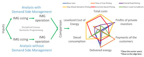
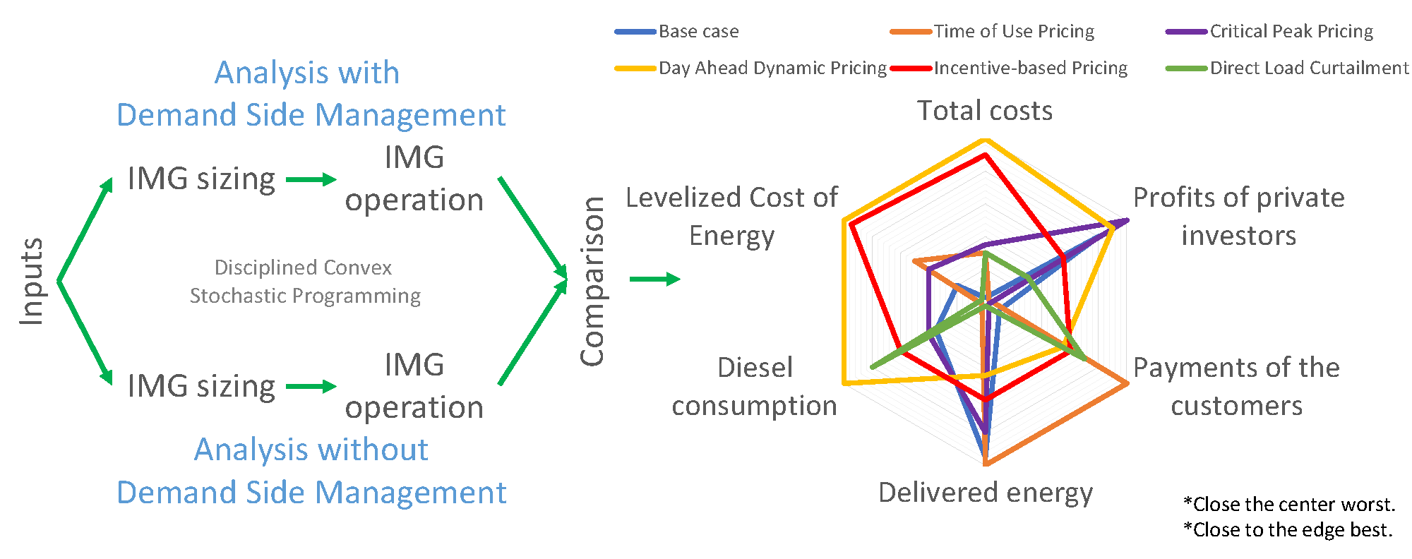
  • Obtaining the optimal sizing and the optimal energy dispatch strategy of an IMG project using a Disciplined Convex Stochastic Programming formulation.
  • Obtaining the optimal energy tariffs and stimulus for the DSM to guarantee the financial viability of an IMG project.
  • Evaluating the impacts of different strategies of DSMs over sizing, energy management, and costs of an IMG project in a case study.
  • Implementing and evaluating different DSMs in the planning of IMGs using the same test-bench.
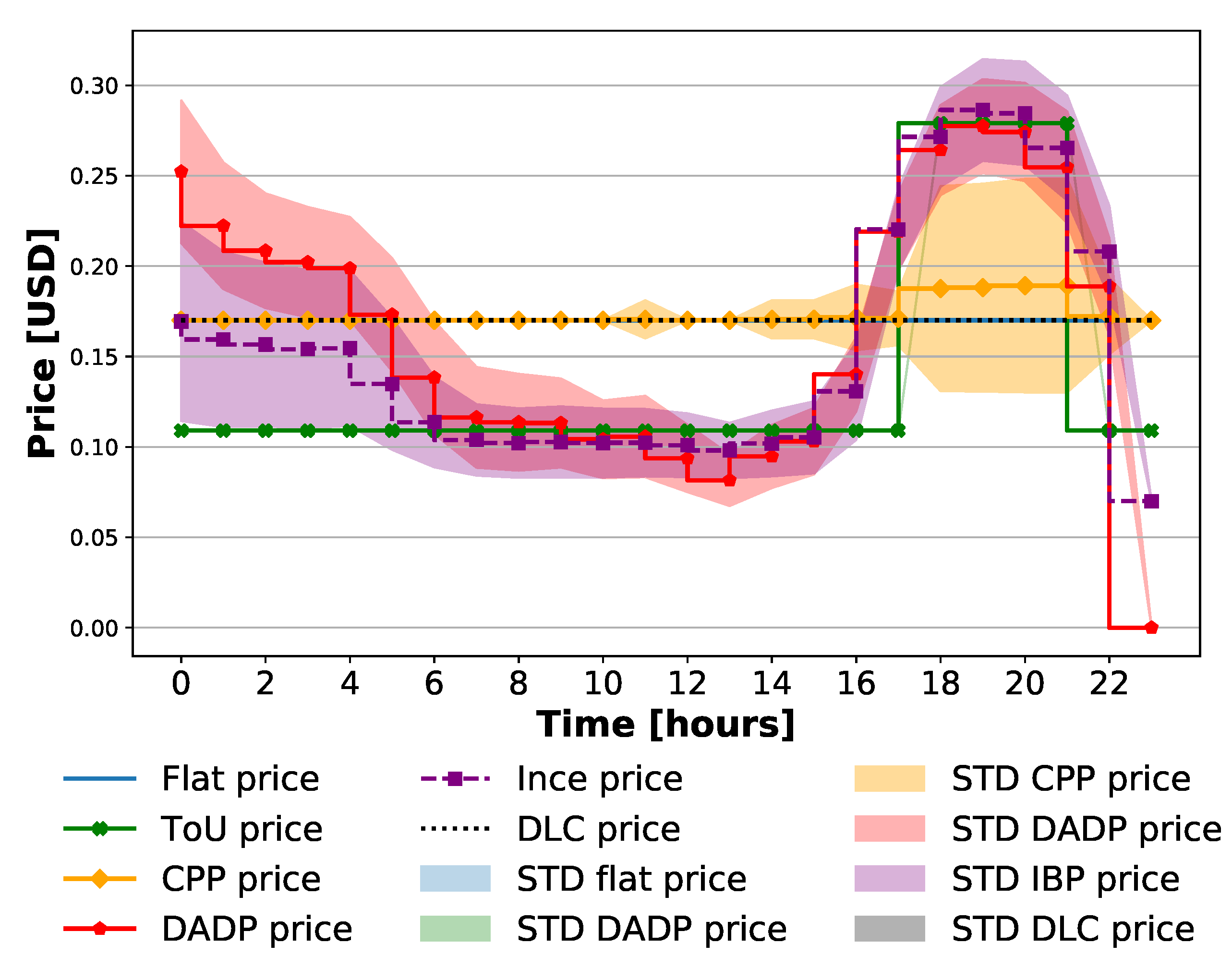
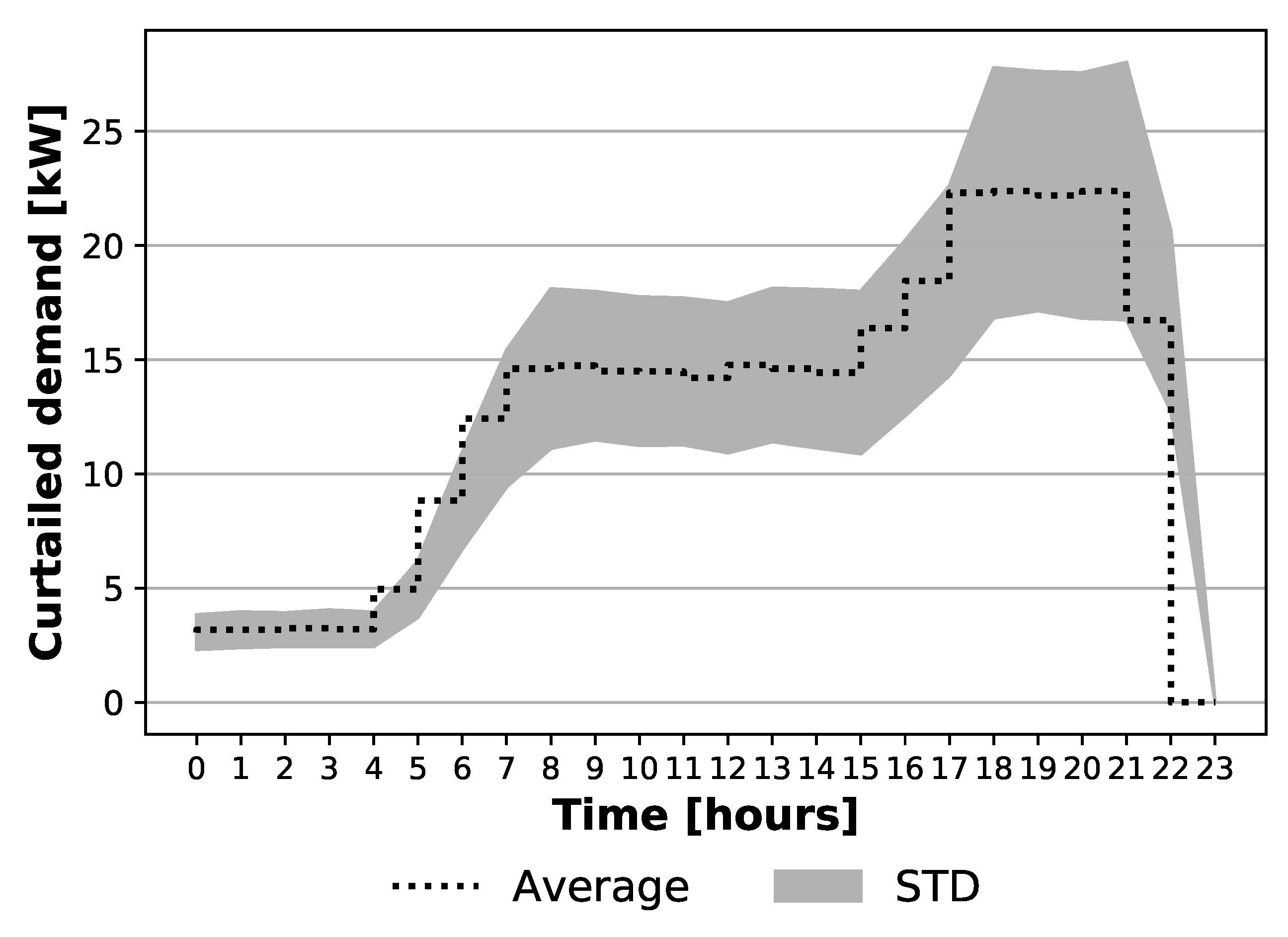
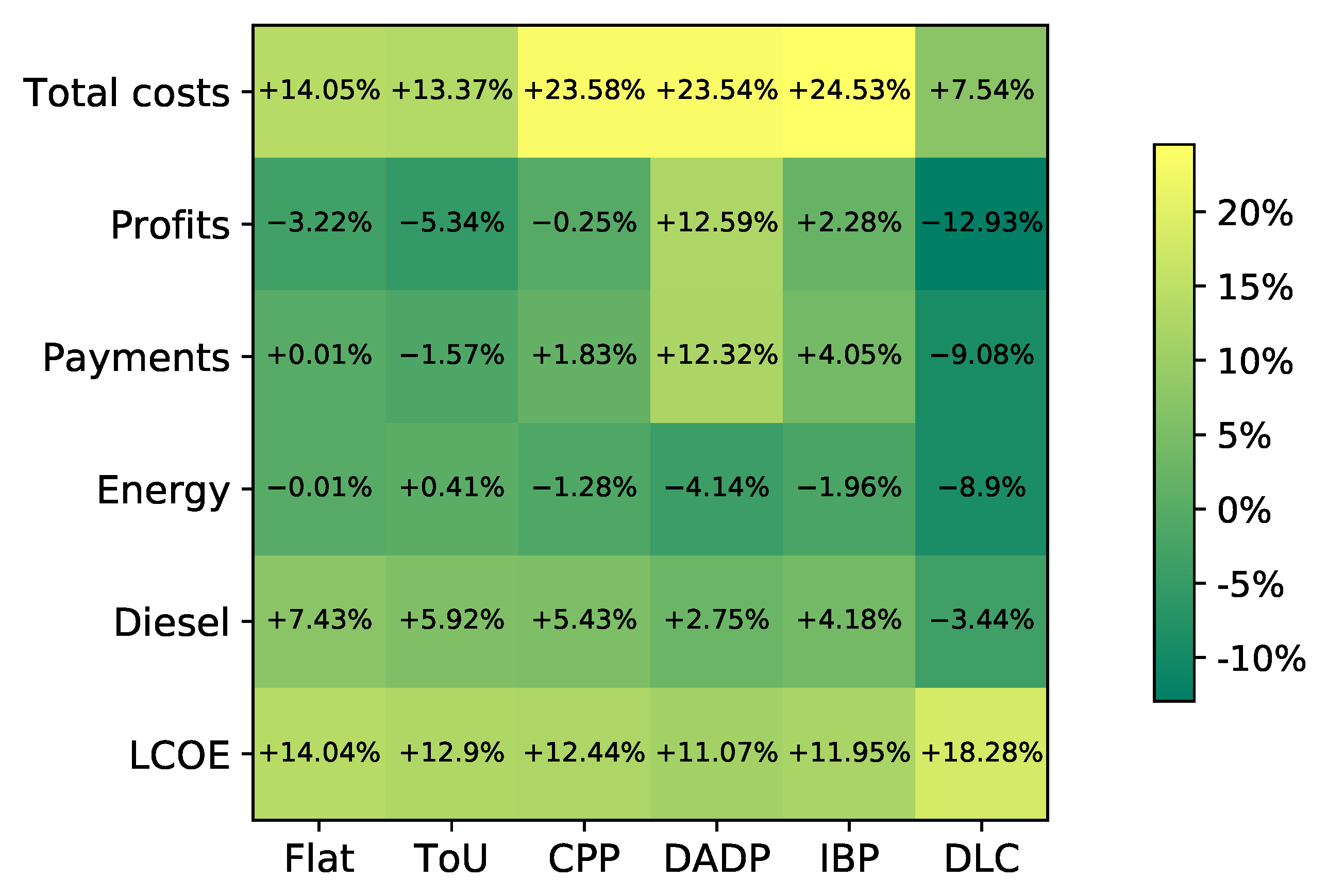
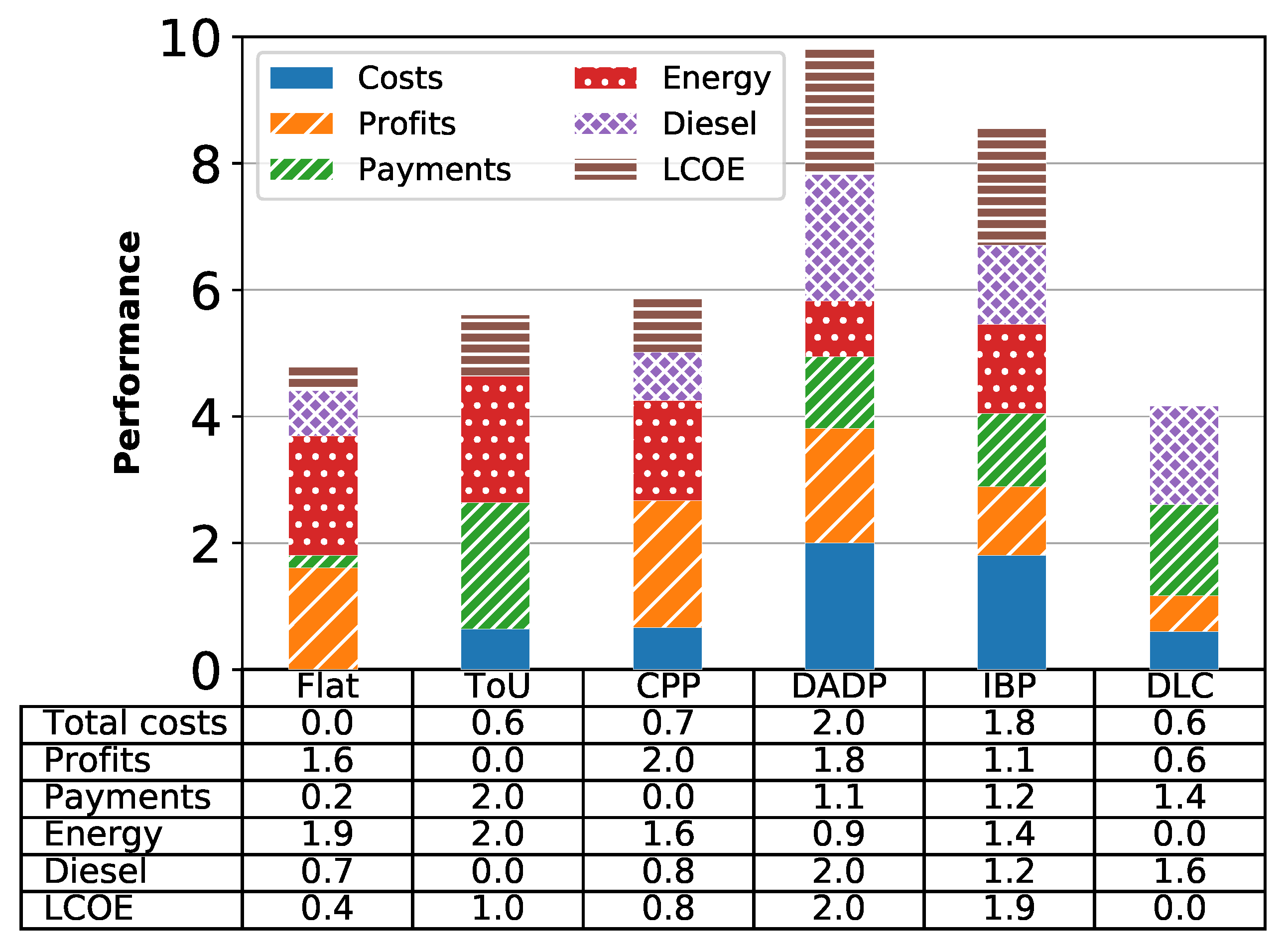
The formulation uses flat, ToU, CPP, DADP, and Incentive-Based Pricing (IBP) tariffs as DSM strategies. It also proposes a Direct Load Curtailment (DLC) strategy that curtails customers’ electrical demand if required.
The formulation assumes that the DSMs modify the patterns of consumption of the customers, which will lead to a change in the capacities of energy sources [36,37,38,39]. The results of the application of the methodology provide the optimal size of the energy sources, the optimal energy dispatch, the optimal tariffs, the economic incentives, and the load curtailment. The rest of the article proceeds as follows: 
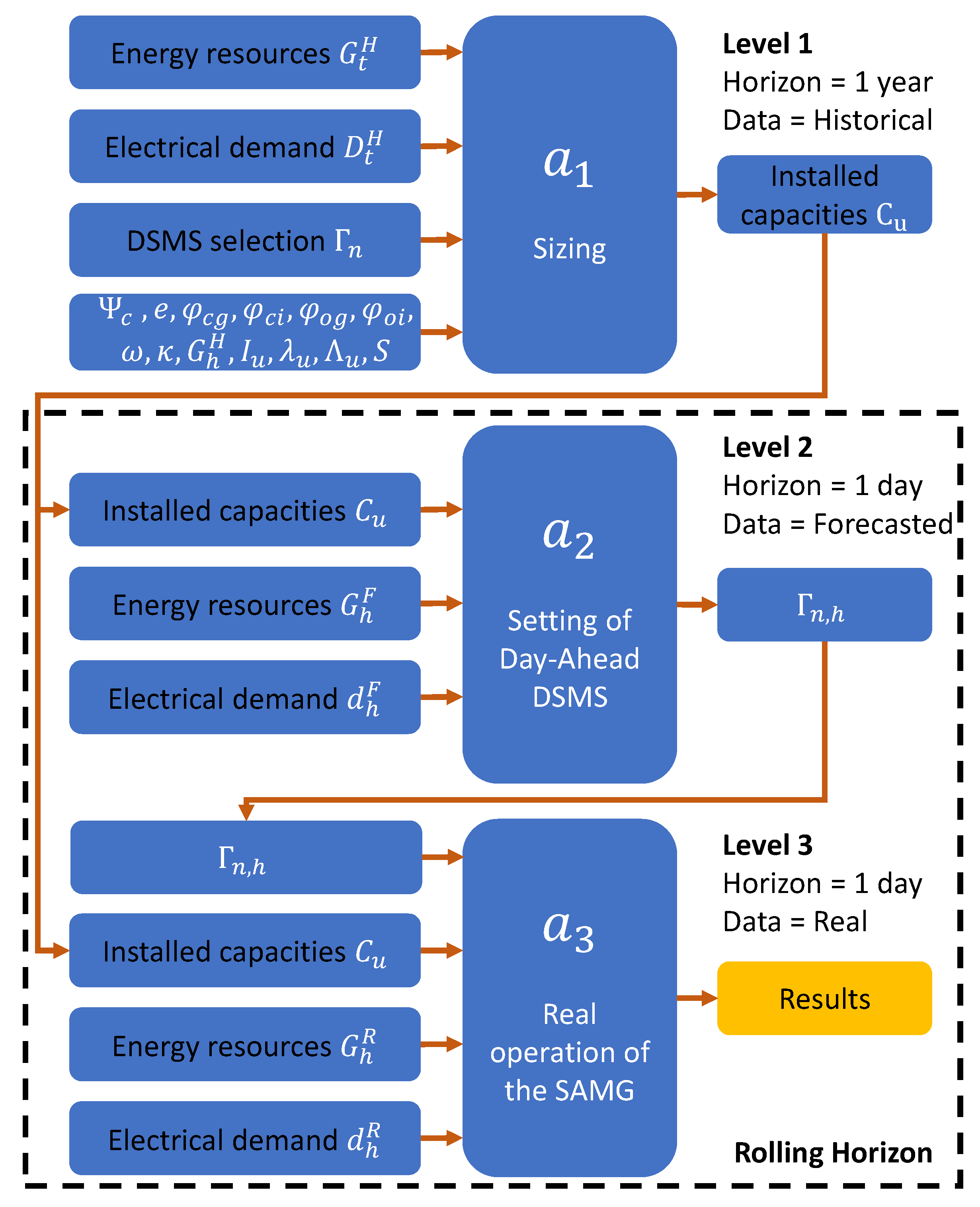
Section 2 presents the definition of the problem and the proposed solution. Section 3 presents a case study as an example of the application of the methodology, and Section 4 includes its results and analysis. Finally, Section 5 presents the conclusions of the work and future directions.
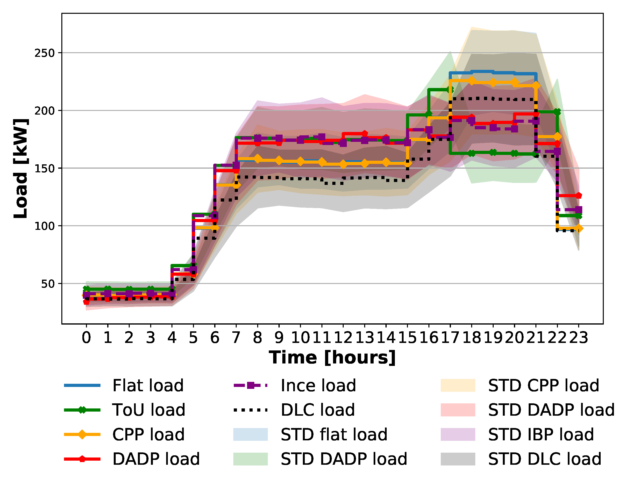
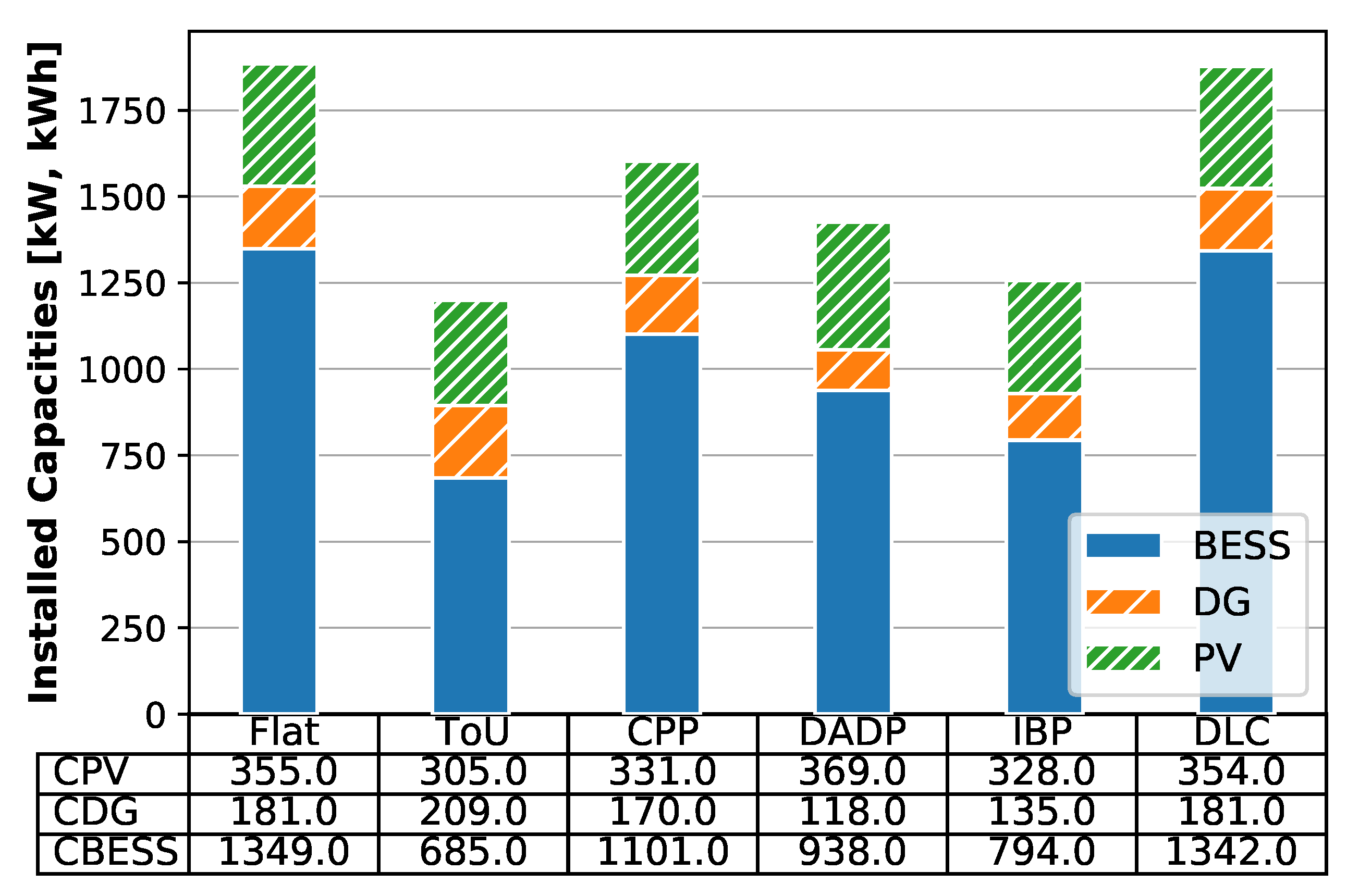
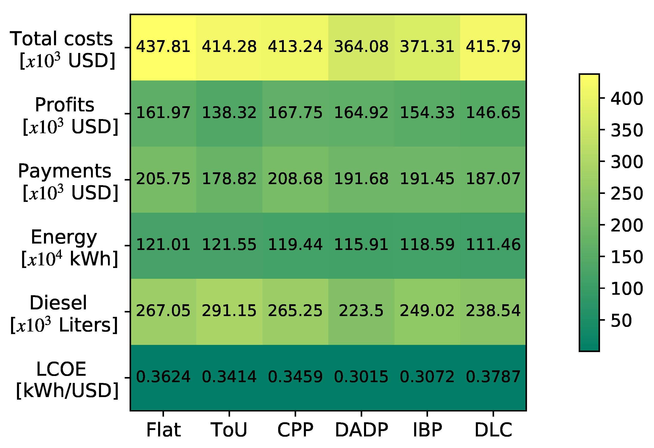
2. Definition of the Problem and Proposed Solution

The present work aims to illustrate for planners and policymakers the benefits of applying DSM for IMG planning. For that purpose, the methodology integrates sizing and IMG operation using three different optimization levels, as shown by Figure 1. The first level obtains the sizes of energy sources using a Monte Carlo analysis. The second level uses a day-ahead rolling horizon over the same optimization horizon of the first level to define incentives, tariffs, and load curtailment of each of the strategies of DSM. Finally, the third level simulates the microgrid operation by iterating in the same rolling horizon that the second level uses. The third level performs the simulation to compute the optimal dispatch strategy after weather and demand profiles are known.
The rolling horizon computes one day in advance at each time and rolls over one year. Each day, the second level computes the proper day-ahead DSM stimulus that the third level uses to compute the day-ahead response of the customers. The second level computes these stimuli using day-ahead forecasts of electrical demand. The third level applies the stimulus found in the second level to compute the customers’ response. While the first and second level assess the uncertainties in day-ahead forecasts of the demand and in weather variables, the third level assumes perfect knowledge of these variables. This assumption allows the methodology to compute the impacts of errors in forecasts over the DSM performance. The formulation computes the total costs of operation on the third level. Section 2.1Section 2.3 present a detailed explanation of each of the levels. Appendix A, present in Table A1 a description of all the variables used in the following sections with their respective names and units.

2.1. First Level: Sizing

The formulation of the first optimization level a 1 can be stated as:
J ( x * ) = minimize x a 1 ( x , ξ ) subject to b i ( x , ξ ) = 0   i = 1 , , B , c i ( x , ξ ) 0   i = 1 , , C ,
where x represents the decision variables, ξ represents the uncertainties of the electrical demand, b i , i = 1 , , B are convex functions in x for each value of the random variable ξ , and c i , i = 1 , , C are deterministic affine functions. Since a 1 , b i , i = 1 , , B and c i , i = 1 , , C are convex on x, the definition of Formulation (1) is a convex optimization problem [40] ([41], Chapter 7).
IMG projects can receive funding from public or private capital. To compute the effects of the funding sources over the total costs, profits, and customer payments, the formulation of a 1 introduces factors φ c g , φ c i , φ o g , and φ o i , where φ c i + φ c g = 1 and φ o i + φ o g = 1 . The formulation of a 1 is designed to minimize the Capital Expenditures (CAPEX) and the Operational Expenditures (OPEX) of the IMG. Equations (2)–(10) describe the formulation of a 1 .
X 1 = arg min C u , E u , t φ c g u = 1 U C u I u + φ o g t = 1 T u = 1 U ( λ u , t + Λ u , t ) E u , t
where the CAPEX ( ζ ) and OPEX ( ϑ ) refer to:
ζ = u = 1 U C u I u
ϑ = t = 1 T u = 1 U ( λ u , t + Λ u , t ) E u , t
and C u , I u , λ u , t , Λ u , t , and E u , t represent the installed capacity, unitary investment cost, unitary dispatch costs, unitary maintenance costs, and dispatched energy by the u energy source, respectively.
It is worth noting that the formulation of Equation (2) replaces m i n i m i z e with a r g m i n , and assigns the results to the variable X 1 . This replacement occurs because the second and third methodology levels require the values of the decision variables, but not the value of the achieved minimum. The rest of the optimization formulations in the document maintain the replacement.
The proposed formulation considers the energy prices as the only revenue stream for the investors. Equation (5) introduces a constraint to guarantee that the private investors recover their investments and the expected Internal Rate of Return R.
( φ c i ζ + φ o i ϑ ) ( 1 + R ) + t = 1 T π n , t D f , t 0
where φ c i and φ o i represent the percentage of payments of the private investor for the CAPEX and OPEX costs, and π n , t represents the prices of the n tariff. Equation (6) considers the elasticity ( e t ) of the customers at a time t, the initial price of the energy ( π f l a t ), and the initial demand ( D o , t ) to compute the final demand ( D f , t ). Equation (7) introduces an energy conservation factor Ψ c to define how the total energy consumption over the optimization horizon changes after the introduction of DSM. Values of Ψ c 1 decrease the total energy consumption, while values of Ψ c 1 increase the total energy consumption over the optimization horizon. A value of Ψ c = 1 indicates that the total energy consumption over the optimization horizon remains constant after the introduction of DSMs.
e t = π f l a t ( D f , t D o , t ) D o , t ( π n , t π f l a t )
t = 1 T D f , t Ψ c t = 1 T D o , t = 0
The formulation of a 1 also includes the energy balance Equation (8), a constraint that limits energy excess ( E E t ), and a constraint that limits the lack of energy ( L E t ), (9) and (10), respectively. Equations (9) and (10) introduce the parameter z to control the desired level of reliability in the IMG.
t = 1 T u = 1 U E u , t E E t + L E t D f , t = 0
t = 1 T E E t ( 1 z ) t = 1 T D f , t
t = 1 T L E t ( 1 z ) t = 1 T D f , t
Additionally, the a 1 formulation includes Equations (14) till (26) in order to evaluate the impact of DSM strategies on the sizing of the IMG (changing the horizon from 24 to 8760 h, respectively).

2.2. Second Level: Setting of Day-Ahead DSM Values

The formulation of the second optimization level a 2 solves the following problem:
X 2 = arg min E u , h F , E E h F , L E h F φ o g h = 1 24 u = 1 U ( λ u , h + Λ u , h ) E u , h F + ω E E h F + ω L E h F
s . t . h = 1 24 u = 1 U E u , h F E E h F + L E h F d f , h F = 0 ,
where E E h F and L E h F are the 24 day-ahead forecasted energy excess (a non-positive variable) and the forecasted lack of energy (a non-negative unrestricted variable), respectively, and ω is a penalization factor. E u , h F and d f , h F represent the 24 day-ahead forecasted dispatch of the u energy sources and the 24 day-ahead forecasted electrical demand, respectively.
The formulation of the second optimization level a 2 uses the capacities C u , the day-ahead forecasts of energy resources G h F , and forecasts of electric demand d o , h F as inputs in order to compute the day-ahead stimulus for the five Γ n , h DSM strategies. Four of the DSM strategies use π n in Equation (5) as an indirect stimulus to modify the customer consumption patterns. Those four DSM strategies are: Time of Use pricing (ToU), Critical Peak Pricing (CPP), Day-Ahead Dynamic Pricing (DADP), and Incentive-Based Pricing (IBP). The last DSM uses a Direct Load Curtailment strategy that sheds a percentage of load when required. The baseline case for comparisons uses a flat tariff and no DSM. The description of the baseline case and each of the DSMs proceeds in the following subsections [42].

2.2.1. Flat Tariff (Baseline Case)

In general terms, the unitary value of a flat tariff is the sum of all the costs of producing the energy divided by the total amount of energy produced [43]. Equation (13) describes the yearly payments using a regular flat tariff.
Θ f l a t = ζ + t = 1 T ϑ t t = 1 T D f , t ( 1 + R ) t = 1 T D f , t
However, this traditional approach does not set an optimal tariff to recover investments while minimizing energy costs. Here, we propose the introduction of a decision variable π f l a t into the formulation to find the optimum price for the tariff.
Θ f l a t = π f l a t t = 1 T D f , t

2.2.2. Time of Use Tariff

ToU tariffs vary daily or seasonally on a fixed schedule, using two or more constant prices [44]. One of the main benefits of this type of tariff is its stability over long periods, which gives the customer a better ability to adapt to it [45,46]. To create a ToU tariff, the planner must define the number of Y blocks and the starting and ending hours of each y block [45]. The optimization problem considers the prices π y of the Y number of blocks as decision variables to be computed. Equation (15) presents the yearly payments using Y different block hours of prices.
Θ t o u = t = 1 T y = 1 Y π y D f , t
The methodology computes the ToU and flat tariffs in the first optimization level a 1 and the demand response of the customers in the third level a 3 . The second level is not used for the flat tariff and the ToU tariff because they do not have daily variations. The algorithm computes the flat and ToU tariffs following the same process used to find the capacities of the energy sources C u , using adapted versions of Equations (30) and (31).

2.2.3. Critical Peak Pricing

The CPP tariff can be 3 to 5 times higher than the usual tariff, but is allowed only a few days per year [46]. In Equation (16), π b a s e is a scalar variable that is chosen to be equal to the flat tariff π f l a t . π p e a k is a decision variable of dimension 24 and is computed one day in advance. Equation (16) defines the day-ahead forecasted payments using a CPP tariff, and Equation (17) defines the day-ahead hourly critical peak price.
Θ c p p F = π b a s e h = 1 τ b a s e d f , h F , b a s e + h = 1 τ p e a k π p e a k , h F d f , h F , p e a k
π c p p , h F = π b a s e + π p e a k , h F
A critical forecasted event, such as high demand or low generation capacity, triggers the critical peak price in a CPP tariff. In this regard, the CPP tariff must include a predictor of the critical event and a decision mechanism to set the value of the critical price. The first optimization level formulation a 1 uses historical data, which implies that the formulation has full knowledge over the optimization horizon (T = 8760 h). The perfect knowledge allows the formulation to state constraint (18), which limits the apparition of the critical price only to a few hours in a year. Equation (18) uses variable φ p e a k to control the number of hours with critical price allowed and δ p e a k to define how many times the base price π b a s e is scaled up. The planner defines φ p e a k δ p e a k , and π b a s e , π p e a k , τ b a s e , and τ p e a k are decision variables that the optimization formulation computes.
t = 1 T π p e a k , t φ p e a k T δ p e a k π b a s e
However, in order to simulate the operation of the IMG, the rolling horizon will only know the forecasts one day in advance. The formulation must define a mechanism to determine the conditions that allow the critical peak price to take place. Thus, it defines the critical event as low daily forecasted primary energy resources (lower than a predefined threshold ϱ ). The decision mechanism sets the day-ahead value of the critical price using the variable π p e a k , h F . Equation (19) describes the mechanism to set the CPPs in the operational phase of the IMG.
π c p p , h F = π b a s e + π p e a k , h F , if h = 1 24 G h F ϱ π b a s e , otherwise

2.2.4. Day-Ahead Dynamic Pricing

DADP refers to a tariff that is announced one day in advance to customers and has hourly variations. This scheme offers less uncertainty to customers than “hour- ahead pricing” or “real-time pricing,” thus allowing them to plan their activities [47,48]. Equation (20) introduces the day-ahead payments under a DADP tariff, using π h F as a decision variable vector of dimension 24.
Θ d a d p F = h = 1 24 π h F d f , h F

2.2.5. Incentive-Based Pricing

The IBP tariff provides discounts in the tariff to the customers to increase the electric energy consumption or an extra fare to penalize it. The planner can decide the IBP base price to be equal to the flat tariff π f l a t to guarantee a constant value each day. Variable π i n c , h F computes the day-ahead hourly incentives and can take positive or negative values. Equation (21) defines the day-ahead payments using the IBP tariff.
Θ i n c F = h = 1 24 d f , h F ( π b a s e + π i n c , h F )
All of the N tariffs must have restrictions to avoid null or excessive pricing. Governments, policymakers, or IMG owners can guarantee fair tariffs to the customers with constraint (22).
π n m i n π n π n m a x

2.2.6. Direct Load Curtailment Strategy

The DLC strategy curtails a portion ϵ h F out of forecasted demand if required. The planner of the IMG decides the percentage of curtailed demand κ . The final demand and day-ahead payments are defined as follows:
d f , h F = d o , h F ϵ h F
Θ d l c F = h = 1 24 d f , h F π f l a t
The general restrictions for the DLC strategy are defined as follows:
ϵ h F κ d f , h F
h = 1 24 ϵ h F κ h = 1 24 d f , h F

2.3. Third Level: Real Operation of the IMG

The formulation of the third optimization level a 3 solves the following problem:
X 3 = arg min E u , h R , E E h R , L E h R φ o g h = 1 24 u = 1 U ( λ u , h + Λ u , h ) E u , h R + ω E E h R + ω L E h R
s . t . h = 1 24 u = 1 U E u , h R E E h R + L E h R d f , h R = 0 ,
where the formulation computes the real dispatch of energy sources using capacities C u , real energy resources G h R , real final electric demand d f , h R , and the energy prices π n of each DSM in order to compute the real dispatch of the U energy sources of the IMG.
In addition to Equations (27) and (28), the formulation of a 3 must include physical restrictions for all the U energy sources used to design the IMG (maximum battery charge and discharge rates, maximum power generator output, amongst others). It is essential to highlight that E E h R and L E h R in the third level refer to energy that generators produce in excess and energy that the generators can not provide, respectively. The first level constrains the allowed quantity of excess (Equation (9)) and lack (10) of energy. The second level uses a penalization factor for these variables (Equation (11)). However, the third level is just an accumulator, a counter of these quantities.

3. Case Study

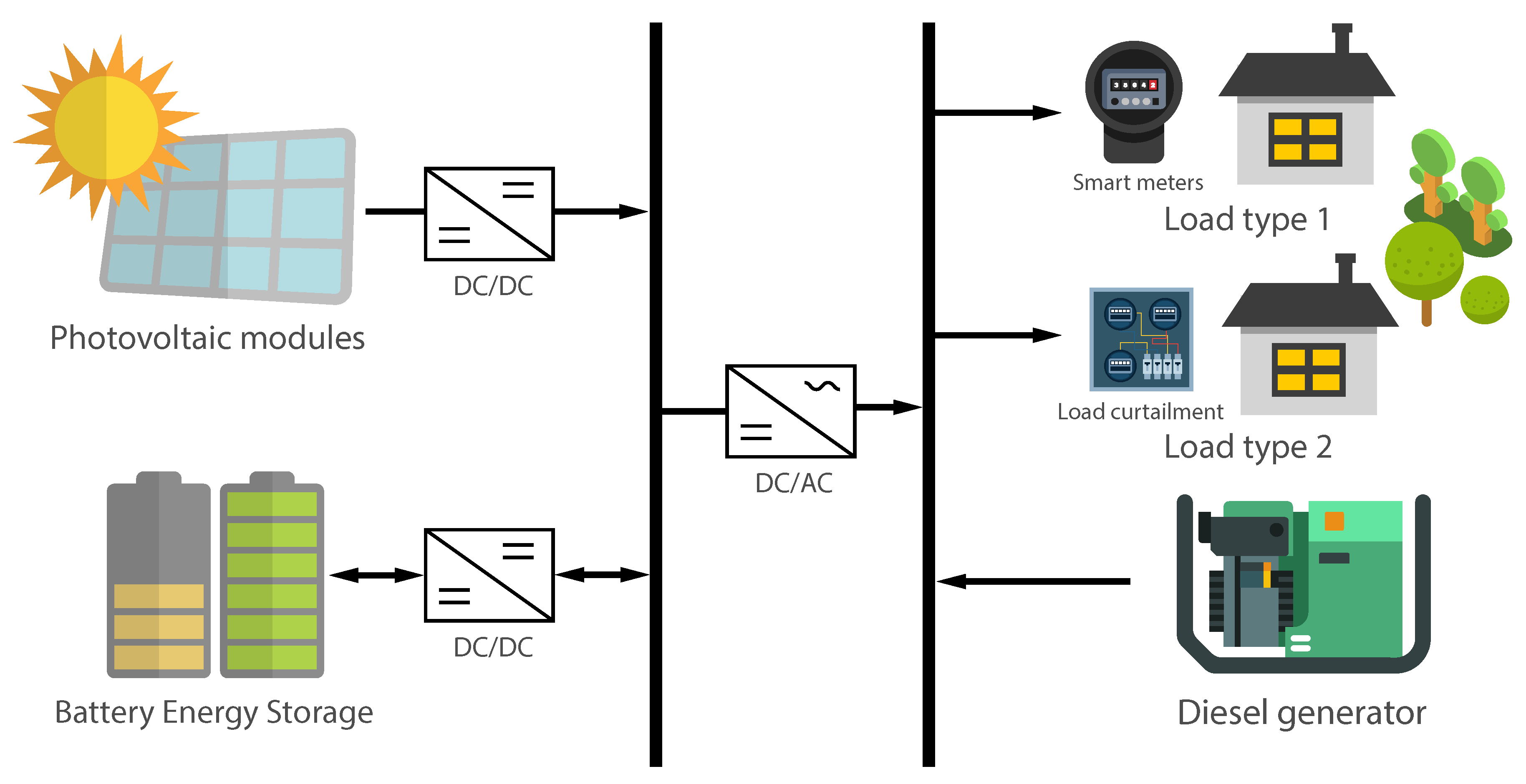
The case study aims to illustrate the capabilities and performance of the proposed methodology and considers the design of an IMG composed of a PV, a BESS, and a Diesel Generator (DG) System, as Figure 2 shows. The case study assumes that the microgrid can have two different types of load. The case study uses the load type one when the planner chooses a DSM based on price. The load type one has Smart Meters. The case study uses the second type of load when the planner decides to use the DSM based on DLC. The second type of load has a device as “GridShare” to perform the curtailment of the electrical demand [31]. The case study considers six IMG designs: Baseline case (flat tariff and no DSM) and one design for each of the proposed DSM (ToU, CPP, DADP, IBP, DLC). The results of the designs using DSM are compared with the baseline case design. All of the optimization formulation was written in Python 3.7 using the CVXPY 1.0 package [49,50]. The selected solver is MOSEK, due to its flexibility, speed, and accuracy [51,52].
The case study includes a Monte Carlo Sampling (MCS) approach to deal with the uncertainties of the stochastic formulation. The MCS approach builds different scenarios by sampling the Probability Distribution Functions (PDFs) of electrical demand. In order to build scenarios, a pre-processing step fits the historic electrical demand into monthly/hourly PDFs. For simplicity and for the sake of reduction in computational burden, the case study assumes the demand follows a Gaussian process without a covariance matrix. Afterwards, a random sampling process of the monthly/hourly PDFs builds the demand for each sample s of the MCS approach. Equation (29) describes the sampling process. Figure 3 shows monthly/hourly fitted distributions using a continuous line to represent the mean and a shaded area to represent the standard deviation.
D t | m , h f ( ψ m , h )
In Equations (2), (11) and (27), X 1 , X 2 , and X 3 represent the S solutions of minimizing a 1 , a 2 , and a 3 , respectively. The C u capacities of the energy sources selected for the IMG in the first level must supply 95 % of the S electrical demands with z level of reliability (as defined by Equation (10)). A post-processing step fits the C u results to a PDF ϕ u , and obtains the Cumulative Distribution Function (CDF) Φ u . The evaluation of the inverse of the CDF Φ u at 0.95 provides the values of energy source capacities C u . These values will supply electrical demand with the desired reliability level 95 % of the time ( 95 % of all the scenarios).
Φ u = ϕ u d C u
C u = Φ u 1 ( 0.95 )

Geographic and Weather Conditions of the Case Study

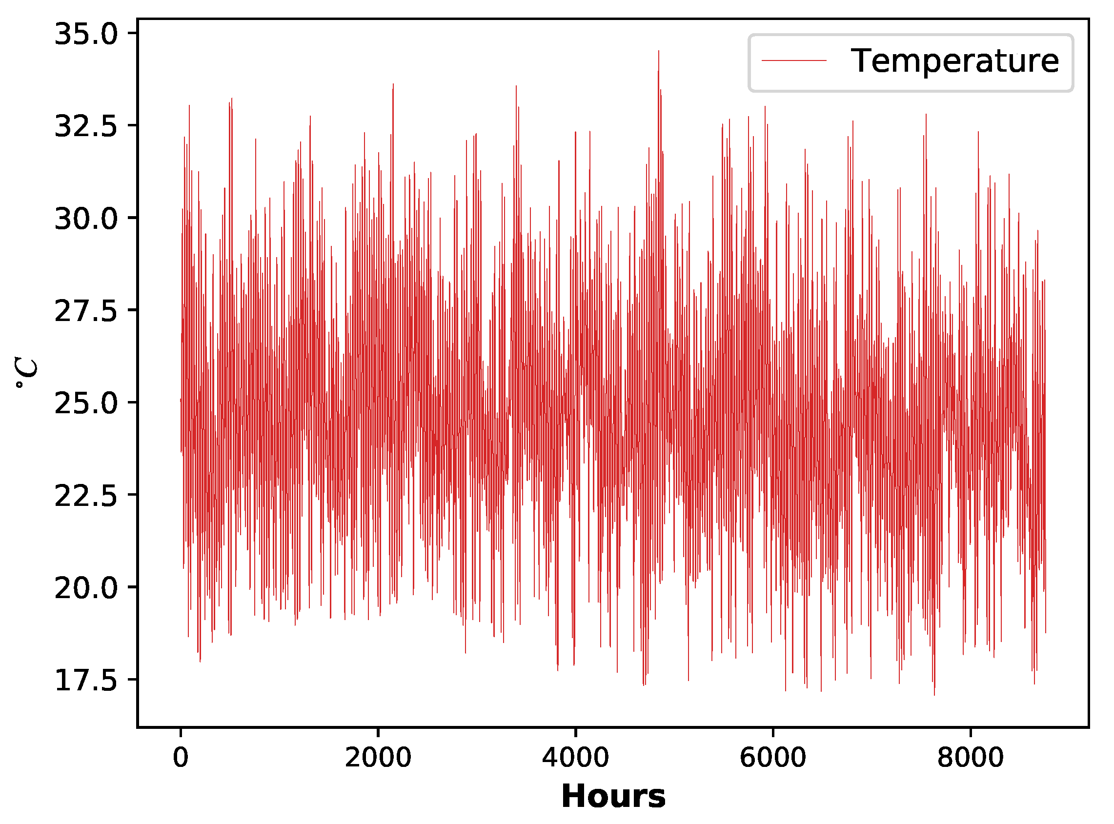
The case study is located at longitude 77 16 8 West and latitude 5 41 36 
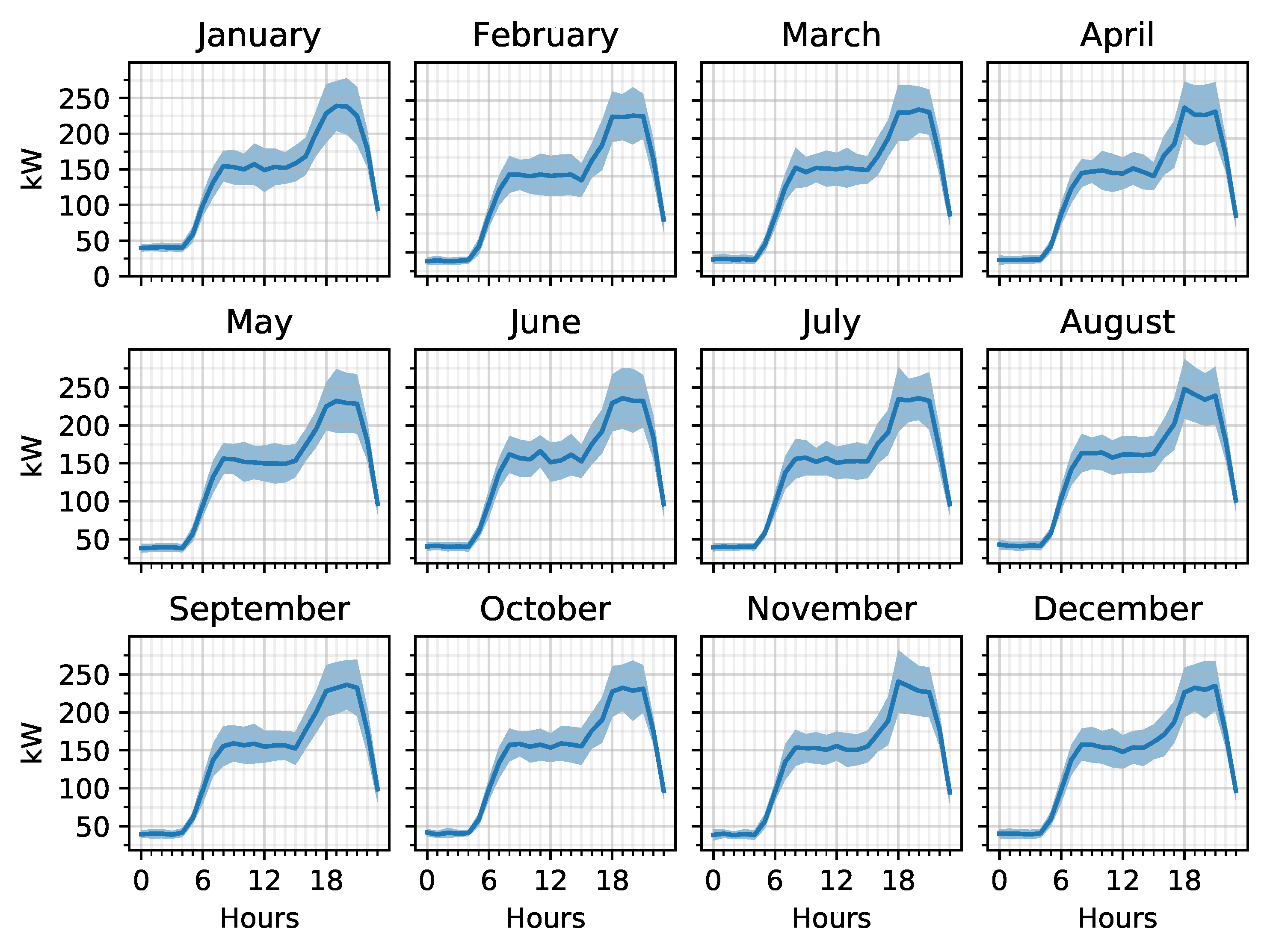
North (Nuquí, Colombia). The study case uses the Meteonorm database of the PvSyst software to obtain the Global Horizontal Radiation (GHI) and temperature conditions of the geographical region. Additionally, the study case uses Homer Pro software to obtain a standard community electrical demand. The standard community electrical demand that Homer Pro provides has hourly steps over a one-year horizon. Figure 4 shows the historic yearly standard profile of the electrical demand that Homer Pro provides. Figure 5 shows the yearly GHI. Figure 6 shows the yearly temperature.
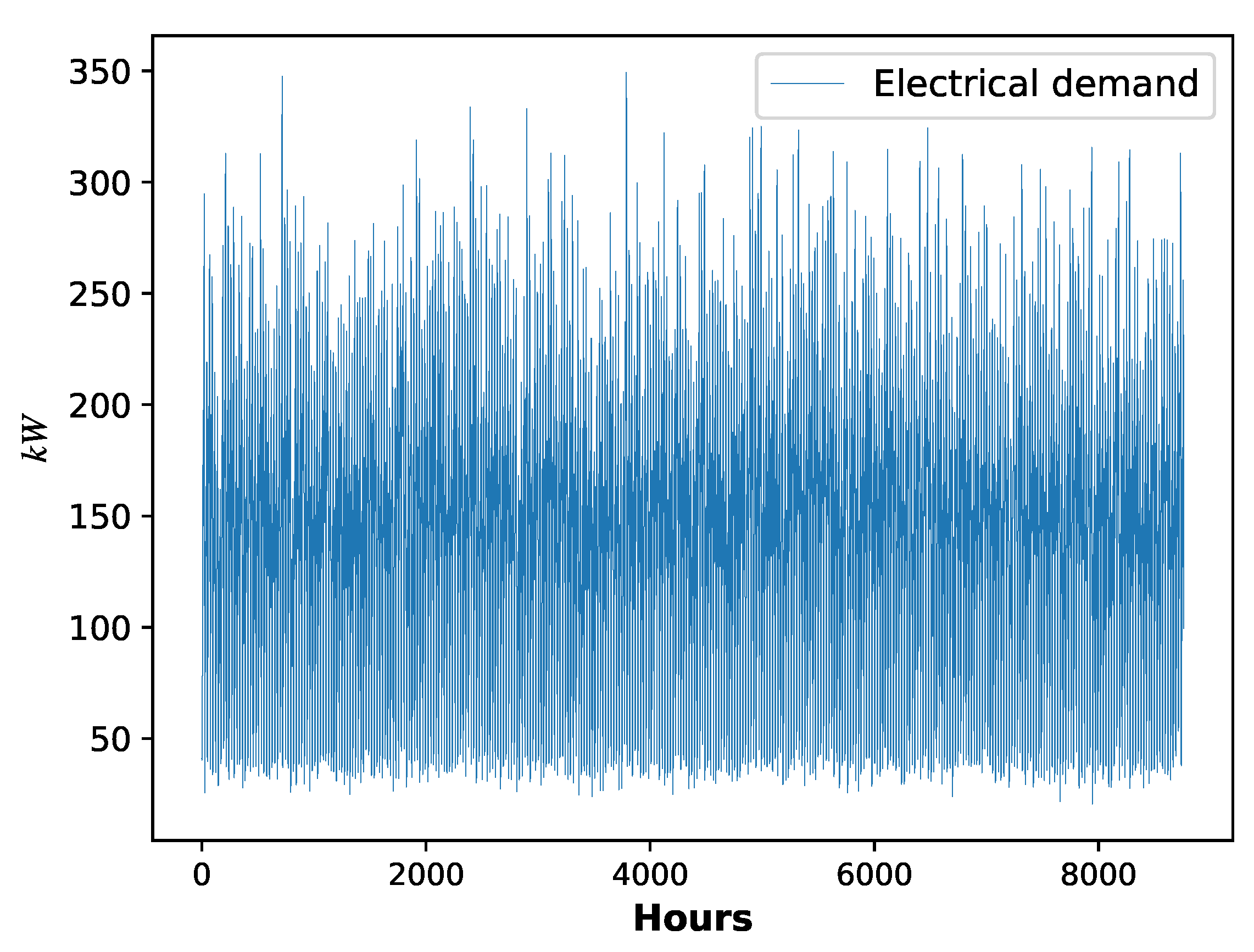
The Monte Carlo Sampling analysis shown in Equation (29) builds the scenarios for the stochastic analysis using the standard community electrical demand obtained from Homer Pro (shown in Figure 4) and a scale factor of 20. The cost of diesel used for the optimization is 0.75 USD/liter. The case study takes the Diesel Generator model from [53], the PV system model from [54,55,56], and the BESS model from [57]. Table 2 summarizes the unitary installation and maintenance costs of the equipment obtained from regional providers. The values assigned to π n , m i n and π n , m a x in constraint (22) are 0 USD/kWh, and two times the price of the current flat tariff of urban areas in Colombia, 0.34 USD/kWh, respectively [58].
Additionally, the methodology takes as inputs the values of Ψ c , e, φ c g , φ c i , φ o g , φ o i , ω , κ , G h H , I u , λ u , Λ u , and S. Planners or policymakers can decide these values or perform sensitivity analyses over each of them. Table 3 shows the values used for simulations in this work. The following section uses the MCS approach and the inputs of Table 3 to compute the results and for the case study.

4. Results and Analysis

The case study aims to evaluate the effects of five different DSMs over the optimization results of the proposed formulation. The five considered DSMs are ToU, CPP, DADP, IBP, and DLC. The study case evaluates different aspects of the effects of the DSMs. Section 4.1 shows the average of each of the tariffs and the curtailment of the DLC strategy. Section 4.2 shows the effects of the DSMs over the sizing of the energy sources of the IMG. Section 4.3 aims to analyze the impacts of the DSMs over the economic aspects of the microgrid. This section analyzes the impacts of DSMs over total costs, profits of private investors, customer payments, and LCOE. Additionally, the section considers the delivered energy and fuel consumption. Section 4.4 presents the effects of the forecast errors over the operation of the IMG. Section 4.5 presents percentage variations in crucial indicators as total cost of the project and LCOE between the first and the third optimization levels. Finally, Section 4.6 shows a comparison of the performance of all the DSMs.

4.1. Demand Side Management Analysis

Each of the Γ n DSM strategies uses a different stimulus to modify customer consumption patterns. Γ T o U , Γ C P P , Γ D A D P , and Γ I B P use tariffs as an indirect stimulus to modify those patterns. Figure 7 shows the average daily stimulus and the Standard Deviation (STD) of the DSMs. The lines represent daily averages of the DSM strategies, and shaded area represents STDs.
Figure 7 presents energy prices. It is interesting to notice that IBP and DADP tariffs reduce the energy price in the middle of the day. The reduction occurs due to the presence of photovoltaic generation in the IMG. IBP and DADP DSMs incentivize customers to increase energy consumption when it is cheaper to generate electric energy.
The Γ D L C DSM curtails a percentage of the demand. Figure 8 shows the daily average of the curtailed values in a continuous line and the STD of the curtailed energy in a shaded area.
The stimulus introduced by DSM strategies modifies customers’ consumption patterns. Using Equation (6) and the stimulus computed using Equations (15)–(26), it is possible to compute the demand response. Figure 9 shows the demands after the application of DSM. The lines represent daily averages of the electrical demand, and shaded area represents the STDs.
It is interesting to note in Figure 7 that the IBP rate tends to be similar to the DADP rate. Therefore, it produces similar effects over electrical demand (see Figure 9). The lack of hourly restrictions on the appearance of the incentive of the IBP tariff causes this to occur. However, the design of hourly restrictions will rely on the experience of the IMG planner, which may ultimately lead to sub-optimal results.

4.2. Sizing Analysis

The variations in the customers’ consumption patterns modify the IMG sizing. Figure 10 presents the variations in the sizing of the Diesel Generator, the photovoltaic system, and the BESS for the five DSMs.
On the one side, Figure 10 shows that ToU- and IBP-based DSMs require less installed capacity than the other alternatives. On the other side, Figure 10 shows that DLC and CPP DSMs do not considerably reduce the energy sources’ installed capacities. However, reductions in installed capacities do not necessarily mean that one DSM is better than others. The following sections contribute with different analyses to determine which of the DSMs can be more suitable for IMG applications.

4.3. Economic Analysis

The DSM introduction in the IMG planning modifies total costs, investors’ profits, customers’ payments, total delivered energy, and LCOE, among others. Equations (32)–(36) present how to compute these values, and Figure 11 shows the results for the five DSM strategies and the base case.
Total cos ts = ζ + ϑ
Profits = t = 1 T π n , t D f , t ( φ c i ζ + φ o i ϑ )
Payments = t = 1 T π n , t D f , t
Energy = t = 1 T D f , t | E E f , t | | L E f , t |
LCOE = Energy Total cos ts

4.4. Assessment of the Impact of Forecast Errors

In the operational stage of the IMG, the proposed formulation computes the DSM stimulus using day-ahead load forecasts. Instead of using a particular method to perform the forecasts, the approach adds Gaussian noise to the real demand to build the forecasted demand, as is stated by Equations (37) and (38). This approach allows measurement of the impact of forecast errors over the final results in the third stage (after knowing the real values of the load).
ν N ( μ , σ 2 )
d h F = d h R ν
Thus, this section presents a sensitivity analysis of the impact of forecast errors. By computing the simulations again, considering forecast errors of 0 % , 5 % , 10 % , and 15 % , this approach computes forecast errors using the Mean Absolute Percentage Error. Table 4 relates the percentage of error with the STD used in Equation (37).
It is significant to notice that the reported errors correspond to the average error for all the forecasts of all the simulated scenarios. In the 0% error case, the forecasted demand values are equal to the real values d h F = d h R . The case study found that the methodology is unable to compute the day-ahead stimulus of the DSMs when the forecast errors are near to 20 % ( σ 2 = 0.2512 ).
Figure 12 shows that the impact of the forecast errors in the total costs, the delivered energy, the investors’ profits, the customers’ payments, and the LCOE is not significant. The variation between the case with perfect forecasts and 15 % error in the forecasts is less than 1 % . The DADP tariff presents the highest variation in profits and payments of the customers, which drop 1 % as compared to the case where the forecast errors are zero.

4.5. Assessment of the Relation between the First and Third Optimization Levels

This article presents the design of a methodology to compute the effects of five different DSMs over the sizing of IMGs. However, in order to calculate the energy sources’ capacities, only the first optimization level of the proposed methodology is required. The second and the third optimization level formulations evaluate the performance of the IMG once it is in operation. Figure 13 reveals the percentage variations between the results from the first and third optimization levels for the five DSMs and the base case.
The first level of the proposed methodology uses a scenario approach built upon historical data and considers an optimization horizon of one year. The second and third levels use a scenario approach built upon forecasts to predict DSMs and consider a rolling horizon with an optimization horizon of one day over a year. Figure 13 presents the comparison between the average results from the first and third levels when the error in the forecasts is 10 % . The extra costs, payments, and LCOE, as well as the reductions in profits and payments, are the result of the change of the optimization horizons and the use of historical instead of forecast data. Planners can also compute percentage variations between the first and third levels for different forecast errors and can utilize trends in percentage variations of each of the values to avoid executing the second and third levels of the methodology. Just by executing the first level and considering the percentages’ variations in their calculations will be enough to estimate the total costs of the IMG project.

4.6. Performance Comparison of the Five DSMs

The five DSMs have different performance in different aspects. Equation (39) is adopted to measure the performance of each of the DSMs.
Performance = worst current worst best
Figure 14 shows that DADP and IBP tariffs perform better than the other DSMs. However, these rates require announcing energy prices one day in advance, so customers reorganize their consumption daily. In the context of IMG, hourly variations of the tariffs might not be the best option in some scenarios. In those scenarios, a ToU tariff or CPP tariff can give a satisfying solution as well.

5. Conclusions

The present work proposes a methodology to design and evaluate five DSMs in the planning and operation of IMGs. The methodology allows determination of the optimal size, optimal energy dispatch strategy, and optimal stimulus for the DSMs using a Disciplined Convex Stochastic Programming approach. The work designs and evaluates the effects of the five DSMs using one case study as a test-bench, which makes this work the first attempt to do so in the literature known by the authors.
The proposed methodology can help policymakers design proper regulations for IMG projects that consider the social conditions of customers and private investors. Additionally, the methodology can be useful for IMG planners or entrepreneurs that want to build profitable business models providing energy to isolated communities. In this regard, the methodology allows policymakers to:
  • Compute the effects of applying one of the five DSMs over the total costs of IMG projects in the planning phase.
  • Control the revenue of private investors or entrepreneurs to prevent excessive profits.
  • Minimize the total amount of subsidies paid by the government for IMG projects.
  • Compute the effects over the sizing and the total costs of IMG projects for different values of customer elasticities.
Additionally, the methodology allows IMG planners or entrepreneurs to:
  • Compute the expected expenses and revenues of an IMG project considering any of the five DSMs.
  • Compute the sizing of the energy sources considering any of the five DSMs.
  • Consider the effects of using different combinations of energy sources to supply the electrical demand.
  • Obtain the optimal day-ahead energy dispatch strategy for the microgrid considering any of the five DSMs.
The methodology can provide the benefits mentioned above to its users if the assumptions that it was built upon are fulfilled. In this regard, by sharpening the assumptions, the methodology will adapt better to the conditions of IMG projects. Considering more energy sources, sophisticated models of customer elasticities, and demand response models adapted to local conditions, among others, will improve the methodology as well.
Finally, it is essential to highlight the technical characteristic of the present study, which aims to inform planners and policymakers about the benefits of applying DSMs in the planning of IMGs. However, policymakers should perform comprehensive social and behavioral studies to evaluate the potential of acceptance of price-based or direct load curtailment DSMs in the context of IMGs.

Author Contributions

Conceptualization, J.C.O.C.; Formal analysis, J.C.O.C.; Funding acquisition, G.O.-P.; Investigation, J.C.O.C.; Methodology, J.C.O.C., R.R., C.D., J.S., and D.H.; Project administration, G.O.-P.; Software, J.C.O.C.; Supervision, C.D.-G. and J.S.; Validation, J.C.O.C., R.R., J.S., and D.H.; Writing—original draft, J.C.O.C.; Writing—review and editing, J.C.O.C., R.R., Cesar Duarte, J.S., and Daniel Hissel. All authors have read and agreed to the published version of the manuscript.

Funding

Administrative Department of Science, Technology, and Innovation (Departamento Administrativo de Ciencia, Tecnología e Innovación)-COLCIENCIAS, Contracts No. 80740-191-2019 and FP44842-450-2017 (ECOS-NORD).

Acknowledgments

The authors wish to thank the Department of Electrical, Electronics, and Telecommunications Engineering (Escuela de Ingenierías Eléctrica, Electrónica y de Telecomunicaciones) of the Vice-Rectorate for Research and Extension (Vicerrectoría de Investigación y Extensión) from the Universidad Industrial de Santander (Project 8593).

Conflicts of Interest

The authors declare that they have no known competing financial interests or personal relationships that could have appeared to influence the work reported in this paper. The funders had no role in the design of the study; in the collection, analyses, or interpretation of data; in the writing of the manuscript, or in the decision to publish the results.

Abbreviations

The following abbreviations are used in this manuscript:
DSMDemand-Side Management
MGMicrogrid
IMGIsolated/Islanded Microgrid
LCOELevelized Cost of Energy
BESSBattery Energy Storage System
PVPhotovoltaic
DGDiesel Generator
MILPMixed Integer Linear Programming
MINLPMixed Integer Non-Linear Programming
CAPEXCapital Expenditures
OPEXOperational Expenditures
MCSMonte Carlo Sampling
PDFProbability Distribution Function
CDFCumulative Distribution Function
STDStandard Deviation
ToUTime of Use
CPPCritical Peak Pricing
DADPDay-Ahead Dynamic Pricing
IBPIncentive-Based Pricing
DLCDirect Load Curtailment

Appendix A

Table A1. Variable declaration.
First stage optimization variables
a 1 Optimization formulation of the first stageUnitless
φ c i Percentage of the CAPEX paid by the investorUnitless
φ c g Percentage of the CAPEX paid by the governmentUnitless
φ o i Percentage of the OPEX paid by the investorUnitless
φ o g Percentage of the OPEX paid by the governmentUnitless
X 1 Results of the optimization formulations of the first stageUnitless
tHour of optimizationHours
TTotal number of hours to optimizeHours
uSpecific generator or storage system of the microgridUnitless
UTotal number of generators and storage systems of the microgridUnitless
nSpecific DSMUnitless
NTotal number of DSMsUnitless
C u Installed capacity of the u devicekW, kWh
I u Unitary initial investment of the u deviceUSD/kW
λ u Unitary costs of generation of the u deviceUSD/kWh
Λ u Unitary maintenance costs of the u deviceUSD/kWh
E u , t Quantity of energy delivered with the u devicekWh
ζ Total capital expendituresUSD
ϑ Total operational expendituresUSD
RInternal Rate of Return for the investorsUnitless
π n , t Price of the n tariff scheme at time tUSD/kWh
D f , t Final electrical demand of the communitykWh
e t Self-elasticity of the customersUnitless
π f l a t Flat tariffUSD/kWh
D o , t Initial electrical demand of the communitykWh
Ψ c Electric energy conservation factorUnitless
E E t Amount of energy in excesskWh
L E t Lack of energy to fulfill the demandkWh
zReliability levelUnitless
Second stage optimization variables
a 2 Optimization formulation of the second stageUnitless
X 2 Results of the optimization formulations of the second stageUnitless
hHours of the dayHours
E u , h F Quantity of forecasted delivered energy with the u devicekWh
E E h F Amount of forecasted energy in excesskWh
L E h F Lack of forecasted energy to fulfill the demandkWh
ω Penalization factorUnitless
d f , h F Final electrical day-ahead forecasted demand of the communitykWh
Θ f l a t Payments with flat tariffUSD
Θ t o u Payments with ToU tariffUSD
ySpecific hourly block of the ToU tariffUnitless
YTotal number of hourly blocks of the ToU tariffUnitless
π y Price at hour y of the ToU tariffUSD/kWh
Θ c p p F Day-ahead forecasted payments of the customers under the CPP tariffUSD
π b a s e Base price of the CCP tariffUSD/kWh
τ b a s e Time under base price for the CPP tariffHours
d f , h F , b a s e Forecasted final electrical demand at base pricekWh
τ p e a k Time under peak price for the CPP tariffHours
π p e a k , h F Forecasted peak price of the CCP tariffUSD/kWh
d f , h F , p e a k Forecasted final electrical demand at peak pricekWh
π c p p , h F Forecasted Critical Peak Price tariffUSD/kWh
π p e a k , t Peak price of the CCP tariffUSD/kWh
φ p e a k Percentage of the horizon T allowed to have a peak priceUnitless
δ p e a k Times that π b a s e is scaled in the CPP tariffUnitless
G h F Global horizontal solar radiationW/m 2
ϱ Threshold to trigger the CPP pricekW/m 2
Θ d a d p F Day-ahead forecasted payments of the customers under the DADP tariffUSD
π h F Forecasted hourly price of the DADP tariff schemeUSD/kWh
Θ i n c e F Day-ahead forecasted payments of the customers under the incentive-based tariffUSD
π i n c e , h F Forecasted incentive price of the IBP tariffUSD/kWh
π n , m i n Minimum value of the n tariffUSD/kWh
π n Price of the n tariff schemeUSD/kWh
π n , m a x Maximum value of the n tariffUSD/kWh
d o , h F Forecasted initial electrical demandkWh
ϵ h F Forecasted curtailed demandkWh
Θ d l c F Day-ahead forecasted payments of the customers under the DLC DSMUSD
κ Percentage of the electrical demand to curtailkWh
Third stage optimization variables
a 3 Optimization formulation of the third stageUnitless
X 3 Results of the optimization formulations of the third stageUnitless
E u , h R Real quantity of delivered energy with the u devicekWh
E E h R Real amount of energy in excesskWh
L E h R Real lack of energy to fulfill the demandkWh
d f , h R Real final electrical demandkWh
Case study
D t Electrical demand at time tkW
mMonths of the yearUnitless
hHours of the dayHours
ψ m , h PDF of the month m and hour hkW
Φ u CDF of the capacity resultskW
ϕ u PDF of the capacity resultskW
sSpecific scenarioUnitless
STotal number of scenariosUnitless
Υ L Diesel price per literUSD/liter
L u Lifetime of the u technologyYears
L p Lifetime of the IMG projectYears

References

  1. Almeshqab, F.; Ustun, T.S. Lessons learned from rural electrification initiatives in developing countries: Insights for technical, social, financial and public policy aspects. Renew. Sustain. Energy Rev. 2019, 102, 35–53. [Google Scholar] [CrossRef]
  2. Ciller, P.; Lumbreras, S. Electricity for all: The contribution of large-scale planning tools to the energy-access problem. Renew. Sustain. Energy Rev. 2020, 120, 109624. [Google Scholar] [CrossRef]
  3. Edwin, M.; Nair, M.S.; Joseph Sekhar, S. A comprehensive review for power production and economic feasibility on hybrid energy systems for remote communities. Int. J. Ambient Energy 2020, 1–39. [Google Scholar] [CrossRef]
  4. Taebnia, M.; Heikkilä, M.; Mäkinen, J.; Kiukkonen-Kivioja, J.; Pakanen, J.; Kurnitski, J. A qualitative control approach to reduce energy costs of hybrid energy systems: Utilizing energy price and weather data. Energies 2020, 16, 1401. [Google Scholar] [CrossRef] [Green Version]
  5. Zhao, H.; Lu, H.; Li, B.; Wang, X.; Zhang, S.; Wang, Y. Stochastic optimization of microgrid participating day-ahead market operation strategy with consideration of energy storage system and demand response. Energies 2020, 13, 1255. [Google Scholar] [CrossRef] [Green Version]
  6. Wang, Y.; Yang, Y.; Tang, L.; Sun, W.; Zhao, H. A stochastic-CVaR optimization model for CCHP micro-grid operation with consideration of electricity market, wind power accommodation and multiple demand response programs. Energies 2019, 12, 3983. [Google Scholar] [CrossRef] [Green Version]
  7. Wang, Y.; Huang, Y.; Wang, Y.; Yu, H.; Li, R.; Song, S. Energy management for smart multi-energy complementary micro-grid in the presence of demand response. Energies 2018, 11, 974. [Google Scholar] [CrossRef] [Green Version]
  8. Nguyen, A.D.; Bui, V.H.; Hussain, A.; Nguyen, D.H.; Kim, H.M. Impact of demand response programs on optimal operation of multi-microgrid system. Energies 2018, 11, 1452. [Google Scholar] [CrossRef] [Green Version]
  9. Ahmad, S.; Ahmad, A.; Naeem, M.; Ejaz, W.; Kim, H.S. A compendium of performance metrics, pricing schemes, optimization objectives, and solution methodologies of demand side management for the smart grid. Energies 2018, 11, 2801. [Google Scholar] [CrossRef] [Green Version]
  10. Zunnurain, I.; Maruf, M.; Islam, N.; Rahman, M.; Shafiullah, G. Implementation of advanced demand side management for microgrid incorporating demand response and home energy management system. Infrastructures 2018, 3, 50. [Google Scholar] [CrossRef] [Green Version]
  11. Hussain, H.M.; Javaid, N.; Iqbal, S.; Hasan, Q.U.; Aurangzeb, K.; Alhussein, M. An efficient demand side management system with a new optimized home energy management controller in smart grid. Energies 2018, 11, 190. [Google Scholar] [CrossRef] [Green Version]
  12. Wang, Y.; Tang, Y.; Xu, Y.; Xu, Y. A Distributed Control Scheme of Thermostatically Controlled Loads for the Building-Microgrid Community. IEEE Trans. Sustain. Energy 2020, 11, 350–360. [Google Scholar] [CrossRef]
  13. Wang, Y.; Xu, Y.; Tang, Y. Distributed aggregation control of grid-interactive smart buildings for power system frequency support. Appl. Energy 2019, 251, 113371. [Google Scholar] [CrossRef]
  14. Franz, M.; Peterschmidt, N.; Rohrer, M.; Kondev, B. Mini-Grid Policy Toolkit; Technical Report; Alliance for Rural Electrification: Eschborn, Germany, 2014. [Google Scholar]
  15. Reber, T.; Booth, S.; Cutler, D.; Li, X.; Salasovich, J.; Ratterman, W. Tariff Considerations for Micro-Grids in Sub-Saharan Africa; Technical Report February; NREL: Golden, CO, USA, 2018. [Google Scholar]
  16. Casillas, C.E.; Kammen, D.M. The delivery of low-cost, low-carbon rural energy services. Energy Policy 2011, 39, 4520–4528. [Google Scholar] [CrossRef]
  17. Jin, M.; Feng, W.; Liu, P.; Marnay, C.; Spanos, C. MOD-DR: Microgrid optimal dispatch with demand response. Appl. Energy 2017, 187, 758–776. [Google Scholar] [CrossRef] [Green Version]
  18. Kahrobaee, S.; Asgarpoor, S.; Qiao, W. Optimum sizing of distributed generation and storage capacity in smart households. IEEE Trans. Smart Grid 2013, 4, 1791–1801. [Google Scholar] [CrossRef] [Green Version]
  19. Erdinc, O.; Paterakis, N.G.; Pappi, I.N.; Bakirtzis, A.G.; Catalão, J.P. A new perspective for sizing of distributed generation and energy storage for smart households under demand response. Appl. Energy 2015, 143, 26–37. [Google Scholar] [CrossRef]
  20. Kerdphol, T.; Qudaih, Y.; Mitani, Y. Optimum battery energy storage system using PSO considering dynamic demand response for microgrids. Int. J. Electr. Power Energy Syst. 2016, 83, 58–66. [Google Scholar] [CrossRef]
  21. Nojavan, S.; Majidi, M.; Esfetanaj, N.N. An efficient cost-reliability optimization model for optimal siting and sizing of energy storage system in a microgrid in the presence of responsible load management. Energy 2017, 139, 89–97. [Google Scholar] [CrossRef]
  22. Majidi, M.; Nojavan, S.; Zare, K. Optimal Sizing of Energy Storage System in a Renewable-Based Microgrid Under Flexible Demand Side Management Considering Reliability and Uncertainties. J. Oper. Autom. Power Eng. 2017, 5, 205–214. [Google Scholar]
  23. Amir, V.; Jadid, S.; Ehsan, M. Optimal Planning of a Multi-Carrier Microgrid (MCMG) Considering Demand-Side Management. Int. J. Renew. Energy Res. 2018, 8, 238–249. [Google Scholar]
  24. Clairand, J.M.; Arriaga, M.; Canizares, C.A.; Alvarez-Bel, C. Power Generation Planning of Galapagos’ Microgrid Considering Electric Vehicles and Induction Stoves. IEEE Trans. Sustain. Energy 2019, 10, 1916–1926. [Google Scholar] [CrossRef]
  25. Gamarra, C.; Guerrero, J.M. Computational optimization techniques applied to microgrids planning: A review. Renew. Sustain. Energy Rev. 2015, 48, 413–424. [Google Scholar] [CrossRef] [Green Version]
  26. Khodaei, A.; Bahramirad, S.; Shahidehpour, M. Microgrid Planning Under Uncertainty. IEEE Trans. Power Syst. 2015, 30, 2417–2425. [Google Scholar] [CrossRef]
  27. Chauhan, A.; Saini, R.P. Size optimization and demand response of a stand-alone integrated renewable energy system. Energy 2017, 124, 59–73. [Google Scholar] [CrossRef]
  28. Amrollahi, M.H.; Bathaee, S.M.T. Techno-economic optimization of hybrid photovoltaic/wind generation together with energy storage system in a stand-alone micro-grid subjected to demand response. Appl. Energy 2017, 202, 66–77. [Google Scholar] [CrossRef]
  29. Mehra, V.; Amatya, R.; Ram, R.J. Estimating the value of demand-side management in low-cost, solar micro-grids. Energy 2018, 163, 74–87. [Google Scholar] [CrossRef]
  30. Mehra, V. Optimal Sizing of Solar and Battery Assets in Decentralized Micro-Grids with Demand-Side Management. Ph.D. Thesis, Massachusetts Institute of Technology, Cambridge, MA, USA, 2017. [Google Scholar]
  31. Harper, M. Review of Strategies and Technologies for Demand-Side Management on Isolated Mini-Grids; Technical Report; Lawrence Berkeley National Laboratory, Schatz Energy Research Center: Berkeley, CA, USA, 2013. [Google Scholar]
  32. Prathapaneni, D.R.; Detroja, K.P. An integrated framework for optimal planning and operation schedule of microgrid under uncertainty. Sustain. Energy Grids Netw. 2019, 19, 100232. [Google Scholar] [CrossRef]
  33. Luo, X.; Liu, J.; Liu, Y.; Liu, X. Bi-level optimization of design, operation, and subsidies for standalone solar/diesel multi-generation energy systems. Sustain. Cities Soc. 2019, 48, 101592. [Google Scholar] [CrossRef]
  34. Kiptoo, M.K.; Adewuyi, O.B.; Lotfy, M.E.; Ibrahimi, A.M.; Senjyu, T. Harnessing demand-side management benefit towards achieving a 100% renewable energy microgrid. Energy Rep. 2020, 6, 680–685. [Google Scholar] [CrossRef]
  35. Rehman, S.; Habib, H.U.R.; Wang, S.; Buker, M.S.; Alhems, L.M.; Al Garni, H.Z. Optimal Design and Model Predictive Control of Standalone HRES: A Real Case Study for Residential Demand Side Management. IEEE Access 2020, 8, 29767–29814. [Google Scholar] [CrossRef]
  36. Choynowski, P. Measuring Willingness to Pay for Electricity; Technical Report 3; Asian Development Bank: Manilla, Philippines, 2002. [Google Scholar]
  37. Oerlemans, L.A.; Chan, K.Y.; Volschenk, J. Willingness to pay for green electricity: A review of the contingent valuation literature and its sources of error. Renew. Sustain. Energy Rev. 2016, 66, 875–885. [Google Scholar] [CrossRef] [Green Version]
  38. Kim, J.H.; Lim, K.K.; Yoo, S.H. Evaluating residential consumers’ willingness to pay to avoid power outages in South Korea. Sustainability 2019, 11, 1258. [Google Scholar] [CrossRef] [Green Version]
  39. Yevdokimov, Y.; Getalo, V.; Shukla, D.; Sahin, T. Measuring willingness to pay for electricity: The case of New Brunswick in Atlantic Canada. Energy Environ. 2019, 30, 292–303. [Google Scholar] [CrossRef]
  40. Ali, A.; Kolter, J.Z.; Diamond, S.; Boyd, S. Disciplined convex stochastic programming: A new framework for stochastic optimization. In Proceedings of the Thirty-First Conference on Uncertainty in Artificial Intelligence, Amsterdam, The Netherlands, 12–16 July 2015; Number 3 in 31. pp. 62–71. [Google Scholar]
  41. Liberti, L.; Maculan, N. Disciplined Convex Programming. In Global Optimization, from Theory to Implementation; Springer: Berlin/Heidelberg, Germany, 2008; Volume 105, pp. 9455–9456. [Google Scholar] [CrossRef] [Green Version]
  42. Celik, B.; Roche, R.; Suryanarayanan, S.; Bouquain, D.; Miraoui, A. Electric energy management in residential areas through coordination of multiple smart homes. Renew. Sustain. Energy Rev. 2017, 80, 260–275. [Google Scholar] [CrossRef] [Green Version]
  43. Inversin, A.R. Mini-Grid Design Manual (English); Technical Report; World Bank: Washington, DC, USA, 2000. [Google Scholar]
  44. Baatz, B. Rate Design Matters: The Intersection of Residential Rate Design and Energy Efficiency; Technical Report March; American Council for an Energy-Efficient Economy: Washington, DC, USA, 2017. [Google Scholar]
  45. Glick, D.; Lehrman, M.; Smith, O. Rate Design for the Distribution Edge; Technical Report August; Rocky Mountain Institute: Boulder, CO, USA, 2014. [Google Scholar]
  46. Kostková, K.; Omelina; Kyčina, P.; Jamrich, P. An introduction to load management. Electr. Power Syst. Res. 2013, 95, 184–191. [Google Scholar] [CrossRef]
  47. Joe-Wong, C.; Sen, S.; Ha, S.; Chiang, M. Optimized day-ahead pricing for smart grids with device-specific scheduling flexibility. IEEE J. Sel. Areas Commun. 2012, 30, 1075–1085. [Google Scholar] [CrossRef]
  48. Borenstein, S.; Jaske, M.; Rosenfeld, A. Dynamic Pricing, Advanced Metering and Demand Response in Electricity Markets; Technical Report October; University of California Energy Institute: Berkeley, CA, USA, 2002. [Google Scholar]
  49. Liberti, L.; Maculan, N. Global Optimization: From Theory to Implementation; Springer: Berlin/Heidelberg, Germany, 2006; pp. 155–210. [Google Scholar]
  50. Diamond, S.; Boyd, S. CVXPY: A Python-embedded modeling language for convex optimization. J. Mach. Learn. Res. 2016, 17, 1–5. [Google Scholar]
  51. Andersen, E.D.; Roos, C.; Terlaky, T. On implementing a primal-dual interior-point method for conic quadratic optimization. Math. Program. Ser. B 2003, 95, 249–277. [Google Scholar] [CrossRef] [Green Version]
  52. Andersen, E.D.; Andersen, K.D. The Mosek Interior Point Optimizer for Linear Programming: An Implementation of the Homogeneous Algorithm. In High Performance Optimization; Frenk, H., Roos, K., Terlaky, T., Zhang, S., Eds.; Springer: Boston, MA, USA, 2000; Volume 33. [Google Scholar] [CrossRef]
  53. Oviedo Cepeda, J.C.; Khalatbarisoltani, A.; Boulon, L.; Osma-pinto, A.; Antonio, C.; Gualdron, D.; Solano, J.E. Design of an Incentive-based Demand Side Management Strategy for Stand-Alone Microgrids Planning. Int. J. Sustain. Energy Plan. Manag. 2020, 28, 1–21. [Google Scholar] [CrossRef]
  54. Li, B.; Roche, R.; Paire, D.; Miraoui, A. Sizing of a stand-alone microgrid considering electric power, cooling/heating, hydrogen loads and hydrogen storage degradation. Appl. Energy 2017, 205, 1244–1259. [Google Scholar] [CrossRef] [Green Version]
  55. Zhang, J.; Li, K.J.; Wang, M.; Lee, W.J.; Gao, H.; Zhang, C.; Li, K. A Bi-Level Program for the Planning of an Islanded Microgrid Including CAES. IEEE Trans. Ind. Appl. 2016, 52, 2768–2777. [Google Scholar] [CrossRef]
  56. Skoplaki, E.; Palyvos, J.A. Operating temperature of photovoltaic modules: A survey of pertinent correlations. Renew. Energy 2009, 34, 23–29. [Google Scholar] [CrossRef]
  57. Bukar, A.L.; Tan, C.W.; Lau, K.Y. Optimal sizing of an autonomous photovoltaic/wind/battery/diesel generator microgrid using grasshopper optimization algorithm. Sol. Energy 2019, 188, 685–696. [Google Scholar] [CrossRef]
  58. Grupo EPM. Tarifas de Energía Mercado Regulado; Grupo EPM: Medellín, Colombia, 2019. [Google Scholar]
Figure 1. Graphical description of the proposed methodology.
Energies 13 03459 g001
Figure 2. Architecture of the islanded/isolated microgrid of the case study.
Energies 13 03459 g002
Figure 3. Fitting of the electrical demand.
Energies 13 03459 g003
Figure 4. Yearly electrical demand.
Energies 13 03459 g004
Figure 5. Yearly Global Horizontal Radiation.
Energies 13 03459 g005
Figure 6. Yearly temperature.
Energies 13 03459 g006
Figure 7. Daily average price of the selected tariffs.
Energies 13 03459 g007
Figure 8. Daily average load curtailment for the Γ D L C DSM.
Energies 13 03459 g008
Figure 9. Daily average load for each of the DSMs and the base case.
Energies 13 03459 g009
Figure 10. Comparison of the sizing of the energy sources for the DSM against the base case. Diesel Generator and photovoltaic capacities are in kW, and the Battery Energy Storage System (BESS) capacity is in kWh.
Energies 13 03459 g010
Figure 11. Comparison of the costs and the Levelized Cost of Energy (LCOE) of the five DSMs against the base case.
Energies 13 03459 g011
Figure 12. Effects of the forecast errors over the main results. (a) Forecast errors effects for a Critical Peak Pricing (CPP) DSM. (b) Forecast errors effects for a Day-Ahead Dynamic Pricing (DADP) DSM. (c) Forecast errors effects for an Incentive-Based Pricing (IBP) DSM. (d) Forecast error effects for a Direct Load Curtailment (DLC) DSM.
Energies 13 03459 g012
Figure 13. Percentage differences between the results of the first level and the third level for the five DSMs and the base case.
Energies 13 03459 g013
Figure 14. Performance comparison of the base case and the five DSMs
Energies 13 03459 g014
Table 1. Summary of the literature review.
Features2017201820192020Literature GapsProposed Work
Integration of sizing and Demand-Side Management (DSM)[27,28][29,30][32,33][34,35]
Stochastic optimization formulation [32]
Study of subsidies impacts over economic feasibility [33]
Forecasting impacts in the operation [34]
Validation of operation after sizing [35]
Tariff setting for Isolated/Islanded Microgrids (IMGs) for economic feasibility
Utilization of tariffs as DSMs in IMGs
Comparison of different DSMs using one test bench
Influence of public subsidies on tariff setting for IMGs
Table 2. Unitary system costs for simulations.
SystemInitial InvestmentMaintenanceOperation
PV1300 USD/kW60 USD/kW0 USD
BESS420 USD/kWh23 USD/kWh0 USD
DG550 USD/kW30 USD/kWh f ( E D G , t 2 , ψ L )
Table 3. Values of the input parameters for the simulations.
InputValueInputValue
Ψ c 1 κ 10%
e0.3 G h H Figure 5 and Figure 6
φ c g 0.9 I u See Table 2
φ c i 0.1 λ u See Table 2
φ o g 0.9 Λ u See Table 2
φ o i 0.1S100
ω 0.4
Table 4. input parameters for simulations.
Error σ 2 Error σ 2
0%N/A5.01%0.0628
10.01%0.125815.01%0.1881

