Evaluation of the Effective Active Power Reserve for Fast Frequency Response of PV with BESS Inverters Considering Reactive Power Control


Department of Electrical, Electronic and Computer Engineering, University of Catania, 95125 Catania, Italy
*
Author to whom correspondence should be addressed.
Energies 2020, 13(13), 3437; https://doi.org/10.3390/en13133437
Submission received: 17 May 2020
/
Revised: 25 June 2020
/
Accepted: 30 June 2020
/
Published: 3 July 2020
(This article belongs to the Special Issue Assessment of Photovoltaic-Battery Systems)
Abstract
:The increasing presence of distributed generation (DG) in the electrical grid determines new challenges in grid operations, especially in terms of voltage and frequency regulation. Recently, several grid codes have required photovoltaic (PV) inverters to control their reactive power output in order to provide voltage regulation services, and the allocation of a certain amount of active power reserve for fast frequency response (FFR) service during under-frequency contingencies is needed. This requirement involves a significant waste of energy for PV systems, due to the necessity to constantly operate in de-loaded mode, under normal operating conditions. In addition, the variability of the irradiance can affect the correct amount of active power reserve that the system can provide in the moments after an under-frequency occurrence. The increasing number of battery energy storage systems (BESSs), coupled to PV systems, can be used to provide a worthy contribution to this frequency regulation service. The aim of this paper is to analyze the efficiency of active power reserve provided by a BESS connected to the DC bus of a non-ideal grid-connected PV inverter, taking into account the impact of reactive power control. For this purpose, the contribution of BESSs to frequency regulation is discussed and, starting from an existing model of real inverter, an analytical formulation for active power reserve evaluation is presented. Results concerning the impact of reactive power control are also given. Finally, the possibility for a low voltage (LV) grid with aggregated PV systems and BESSs to contribute to grid active power reserve is considered. Different voltage control strategies are compared, defining a helpful new parameter.
1. Introduction
In recent years, the reduction in the carbon intensity of worldwide energy use, known as de-carbonization, has become one of the most crucial objectives for industrialized countries. The European Union has already fixed the deadline for climate neutrality, i.e., no net emissions of greenhouse gasses, at the year 2050, by decoupling the economic growth from the use of resources [1]. In order to achieve this goal, a higher penetration of renewable source power plants in the electric power system is needed. A high potential future contribution can be provided by solar photovoltaic (PV) power plants, reaching a multi-TW scale in 2050 [2] thanks to new technologies and innovative policies [3]. In this field, several projects have been carried out in Italy and in other Mediterranean areas [4,5].
However, the increasing presence of distributed generation (DG) connected to the electric power system is bringing out new challenges in terms of grid and micro-grid (MG) regulation [6,7]. In particular, voltage and frequency issues have a strong impact in grid operation [8,9]. In this scenario, the contribution of PV systems and battery energy storage systems (BESSs) to grid regulation becomes crucial.
Spurred by technology development and regulatory frameworks, self-consumption of distributed renewable electricity generation has gained relevance in many power markets around the world. Building on the concept of “prosumers” (producers and consumers) or “prosumption”, the term “prosumage” has emerged.
Prosumage additionally includes energy storage that can be used to increase self-consumption (producers, consumers and storage). For prosumagers (a prosumager is a “prosumer” who has made additional investments in distributed storage, usually in the form of batteries), the critical service provided by the grid is no longer energy per se but rather balancing services, voltage and frequency support, power quality and, most importantly, service reliability. After all, prosumagers will not cut the cord as they continue to rely on the grid during extended periods when there is no sunlight and their batteries are drained.
Several studies have been conducted in this field, evaluating the participation of PV systems and BESS in voltage and frequency control [10,11,12]. BESSs are able to be opportunely controlled, in order to inject or absorb active power for frequency regulation. This service can be designed in different ways, such as power-frequency droop control, static frequency response and inertia emulation control. A detailed explanation of these kinds of control is given in [13]. In particular, during under-frequency problems in low-inertia power grids, PV systems and BESS can be required to provide a certain amount of active power reserve for fast frequency response [14,15].
Despite participation in this service being available only for large-scale power plants, in [16], the possibility of aggregation of small-scale power plants is explored. The aggregation of distributed plants, able to provide ancillary service, is called Virtual Power Plant (VPP). In particular, coordinated operations of these VPPs can be used by the MG operator in order to provide voltage [17,18] and frequency [19,20,21,22] regulation to the higher level of the grid. In real VPPs, MG operators need to consider how voltage and frequency control influence each other, in order to correctly evaluate the amount of active and reactive power that the VPP can provide to the higher level of the grid. In this scenario, the new figure of “aggregator” is born, defined as the player who manages energy communities in order to trade energy and ancillary services in the energy markets.
In order to correctly evaluate the available active power reserve, the aggregator and active users need to take into account the non-ideality of PV inverters and grid lines, especially when a reactive power regulation strategy is adopted. In fact, when a reactive power control is used in PV inverter, its efficiency is related to the operating power factor (PF). Analogue considerations can be run for real electrical lines, since the reactive power flow causes an increase on the absolute value of line current.
For these reasons, this paper has the following aims:
- Evaluate the effective active power reserve provided by PV systems with BESS, considering the impact of reactive power control strategies used for voltage regulation;
- Evaluate the efficiency of active power reserve provision that VPP can provide at the connection point with the higher level of the grid for frequency regulation, considering grid losses;
- Define a new parameter able to clearly compare the different reactive control strategies in terms of active power reserve efficiency.
Section 2 provides an overview of the Italian Reference Standards for the connection of passive and active users to the electrical grid, with a focus on the required regulation services.
After a description of the adopted models, provided in Section 3, a formulation for evaluating the effective active power reserve of PV inverters is analytically shown in Section 4, starting from the model of non-ideal inverter.
In Section 5, the impact of the reactive power control is evaluated, and the case of a 5-kW PV inverter is studied. The results for a clear-sky day and the impact of clouds are discussed as an example.
The possibility for MG to participate in the frequency regulation service is considered in Section 6 [23,24,25], in which the non-ideality of grid lines is analyzed and a new parameter is defined, in order to make a comparison between different reactive power control strategies, adopted for voltage regulation, in terms of effective active power reserve in the grid.
2. Voltage and Frequency Regulation in Italian Standards
The analysis of voltage and frequency regulation requirements for PV systems with BEES needs a preliminary discussion about the PQ decoupling theory. Considering a generic line h–k of an electrical grid, the active and the reactive power flowing through the line can be expressed as follows [26]:
where
- is the voltage at node h;
- is the voltage at node k;
- is the conductance of the electrical line h–k;
- is the susceptance of the electrical line h–k;
- is the phase between node h and node k.
This mathematical expression is the basis of the analysis of voltage and frequency dependence on active and reactive power.
In HV lines, the conductance can be neglected with respect to the susceptance. For this reason, a separate regulation of frequency and voltage is performed using a decoupling control of active and reactive power, respectively. This consideration is not generally true for LV lines, in which the impact of both active and reactive power on nodal voltage needs to be taken into account.
However, since a combined control is not simple to achieve, Italian Standards CEI 0-21 and CEI 0-16 prescribe active users with a PV system and a BESS to primary control the inverter reactive power during overvoltage events, in order to maintain the nodal voltage below the allowed limit (110% of the rated nodal voltage). When the reactive power control is not sufficient, an adjustment on the active power output is required [27,28,29].
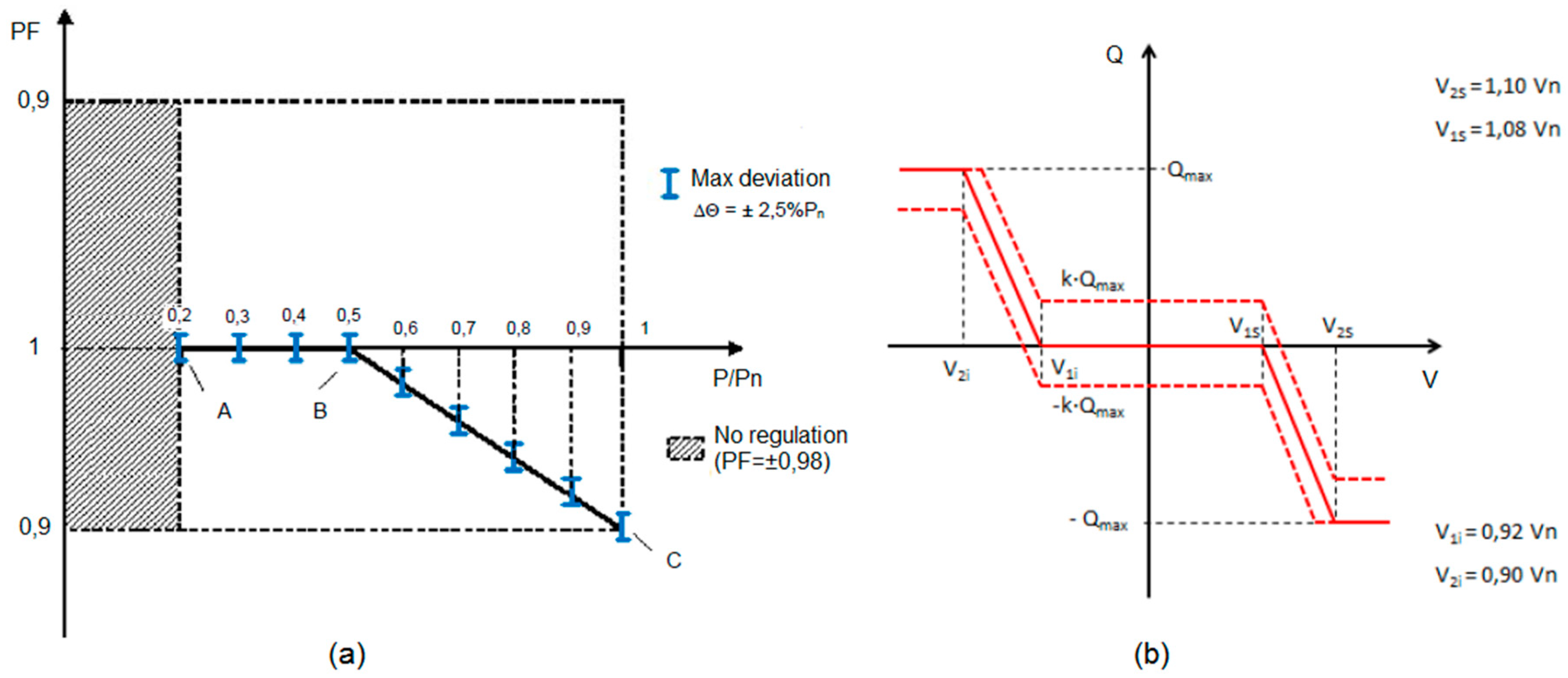
Voltage regulation is performed using an automatic control of inverter reactive power. Two different strategies are proposed in CEI 0-21 and CEI 0-16. In the first strategy, the required values of PF are expressed as a function of the active power. The inverter must follow this regulation curve when the voltage at point of common coupling (PCC) reaches the lock-in value. This value is typically equal to 105% of the rated voltage for overvoltage problems, although an adjustment range, from 100% to 110% of the rated voltage, is required by Italian Standards. Following the PF(P) curve, the inverter continues to provide the output power at PF = 1 until the active power output gets to 50% of the rated active power, (if the lock-in voltage is reached). The PF = f(P) curve is traced by three points (Figure 1a):
- A: , PF = 1;
- B: , PF = 1;
- C: , PF = PF max.
This voltage regulation is disabled when the active power output returns below 50% of (point B), or when the voltage at PCC returns below the lock-in value.
In the other voltage regulation strategy envisaged by Italian Standards, the inverter reactive power output is expressed as a function of the voltage at PCC, defining a Q = f(V) curve (Figure 1b).
Following this regulation curve, the inverter continues to provide the output power at PF = 1 until the voltage at PCC exceeds the normal operation range of [V1i; V1s] if the active power output has reached the lock-in value, typically equal to 20% of . Starting from these points, the inverter reactive power increases (or decreases), according to the curve, until the values V2s or V2i are reached.
This voltage regulation is disabled when the active power output returns below 5% of (lock-out power) or when the voltage at PCC returns within the range [V1i; V1s]. When the active user owns an electrochemical storage system, the parameter k of Figure 1b, varying in the range [−1; 1], could be required by the system operator.
Instead of voltage regulation, Italian Standards prescribe a frequency regulation based on active power control, since active power has a stronger impact on grid frequency than reactive power.
Figure 2 shows the regulation curves for under-frequency and over-frequency problems. The regulation of the active power output is required when the frequency at PCC exceeds the allowed range of [49.8; 50.2 Hz]. It is noticeable that if the system is equipped with a storage system connected to a bidirectional converter, the active user could be required also to absorb active power in over-frequency conditions. The maximum and the minimum values of active power output must be reached at 49.1 and 51.5 Hz, respectively. The working points of Figure 2 represent the generic active power output of the inverter in normal operations at 50 Hz.
When the frequency returns within the range [49.9; 50.1 Hz], the system can end the regulation service and restore its normal operation after a minimum transient time of 300 s.
3. Description of the PV with BESS System Model
The MATLAB/SIMULINK model of a 5kWp PV system, built starting from the one-diode model of the solar cell and considering the influence of solar irradiance and temperature on the P–V curves [30], is used in this paper. The adopted model, suitable for simulation of complex PV plants, is able to accurately predict the PV output even under non-uniform distribution of solar irradiance and temperature. The accuracy of the model is important for a correct evaluation of the active power available for fast fast frequency reserve service.
Taking into account the contribution of BESSs to the frequency support, the two-constant model of a Li-Ion battery is used in order to build the MATLAB/SIMULINK block of a 48-V battery with a rated capacity of 80 Ah, connected to the DC bus of the PV inverter [31]. Typical values of the electrical components of the equivalent circuit, , , , , and are given in [32]. The state of charge (SOC) is estimated by the Coulomb counting method. This method presents a lack of accuracy for very low or very high values of the SOC. However, this aspect does not affect the results shown in this paper, since SOC limits are usually adopted in order to increase battery life [33,34]. In this study, a depth of discharge (DOD) of 70% and a maximum SOC of 95% are implemented in the battery management system (BMS).
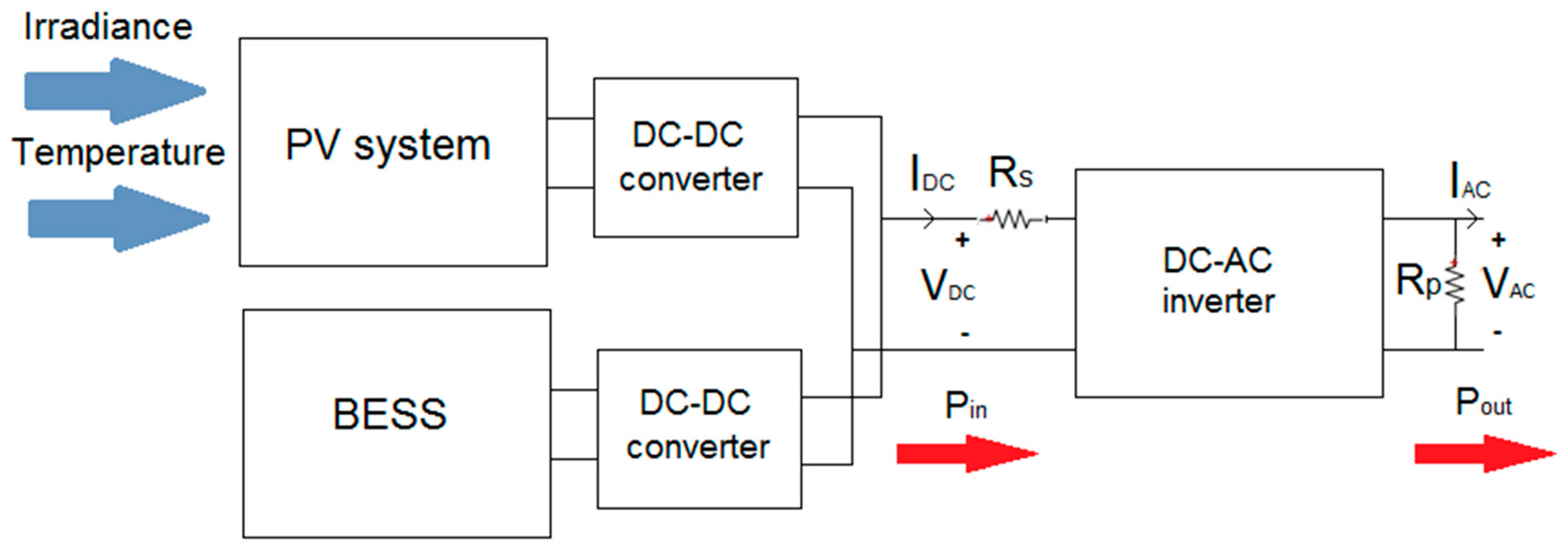
The interface between the PV system and the bus is represented by a two-stage electronic converter, composed of a DC–DC boost converter and a DC–AC inverter [35]. In order to correctly analyze the active power losses of the PV inverter, an accurate, but at the same time simple, model of a real inverter is needed. For this purpose, Chivelet’s model is used in this paper [36]. This model, while being simple and suitable for MATLAB simulations, can evaluate active power losses, taking into account the reactive power produced by the inverter, by the addition of two resistances, (Input series resistance) and (Output shunt resistance) to the ideal model of the inverter (Figure 3).
Starting from the power balance of the DC–AC inverter:
Obtaining from (3), the inverter efficiency can be obtained as a function of the apparent power, S (further details are explained in [37]):
The parameter could be considered equal to 1, except for very low values of the power factor. and represent the voltages at the DC bus and AC bus of the inverter, respectively. In the case of PF = 0, the apparent power, S, can be substituted with the active power, P, in Equation (4).
In [37], values of and for different sizes of inverters are experimentally obtained. Concerning the 5kWp system, the following values are assumed: = 0.8 Ohm and = 4100 Ohm.
The accuracy of the model of each component (PV system, BESS and DC–AC inverter) is specified in the reference literature, in which the root mean square errors (RMSEs) between simulated and measured points are experimentally evaluated. In particular:
- P–V curves: RMSE < 1.5% with uniform distribution of irradiance and temperature and RMSE < 3% with non-uniform distribution of irradiance and temperature [30];
- BESS voltage: RMSE = 2% in continuous discharge condition and RMSE = 1.7% in pulse current discharge condition [31];
- Inverter efficiency: RMSE varies from 1.69% to 3.4% depending on the specific inverter [37].
The high accuracy of each component guarantees an adequate accuracy of the entire system under study.
4. Evaluation of the Effective Active Power Reserve
Due to the necessity of maintaining a certain amount of active power reserve for the fast frequency response (FFR) service, PV systems need to operate in a de-loaded operation mode, below their maximum power point [38]. The amount of active power reserve is defined as a percentage of the active power output of the system:
where is a parameter in the range [0, 1], typically 0.03–0.1, and is the active power at the DC bus of the inverter when = 0.
In PV systems without energy storage, this goal can be obtained by controlling the duty cycle of the DC–DC boost converter, in order to keep the output voltage of the PV system, , higher or lower than the voltage corresponding to the maximum power point, (Figure 4). In fact, the output power, , can be produced in correspondence with two different voltages, and . The active power reserve is represented by the difference between and .
Specific details about the evaluation of the PV power output at the maximum power point are provided in [39,40,41,42], where the use of a second degree polynomial equation, a function of global irradiance and ambient temperature, is proposed and its coefficients are calculated using Villalva’s method [43]. Starting from the estimated maximum power point, , the reference power for the converter, , can be obtained as follows:
where is the required active power reserve, expressed as a percentage of , and is the contribution for the fast frequency response, expressed as a function of the frequency deviation, .
In particular,
with
where is the reference frequency (typically equal to 50 Hz) and is the measured frequency.
Nevertheless, while PV systems can have an unquestionable role in reducing their active power production during over-frequencies, the adoption of this strategy for active power reserve provision in the case of under-frequencies presents two main drawbacks. In order to guarantee the required reserve, the PV system needs to operate in de-loaded mode for all its operation time, causing a non-negligible waste of renewable energy (i.e., a missing revenue for the active user), impacting both economic and environmental aspects. In addition, because of the uncertainty in the prevision of irradiance level, PV systems cannot ensure the exact amount of required active power reserve, especially for low level of irradiance (several grid codes allow PV systems to operate in de-loaded mode only from a certain level of measured irradiance). In fact, Figure 4 gives the P–V curve of the PV system for a specific instance, showing the theoretical amount of its active power reserve. If the PV system is called to inject additional active power in the subsequent milliseconds, a variation in solar irradiance can affect the effective active power that the system can provide. This uncertainty can create stability problems, since the active user cannot guarantee a high level of accuracy regarding the right amount of active power that they can provide during under-frequency events.
For these reasons, since there is an increasing number of active users who own PV systems with combined storage, the BESS can be used for providing the FFR service while the PV system operates at its maximum power point, instead of the de-loaded mode [44,45,46,47]. Further details about feasibility and sizing of BESS for ancillary services are provided in [11,44], where different technologies are compared. In particular, Li-Ion BESSs with typical power output from 0 to 5 MW can guarantee a response time over milliseconds to seconds and they can reach lifespans of 1000–3500 life cycles.
In this case, while the duty cycle of the DC–DC boost converter of the PV system is controlled following a MPPT algorithm, the control of the reference battery power, , implemented in the BMS, can be obtained, starting from (6):
Considering Equation (9), it is noticeable that is null if no FFR service is required, i.e., if the frequency corresponds to its reference values. This configuration has the advantage of avoiding energy waste due to the de-loaded operation mode of the PV system. However, the drawback of this solution is that the BMS does not take into account the reduction on the effective active power reserve due to the non-unitary efficiency of the PV inverter.
Clearly, when Equation (4) is considered, the analysis of the effective active power provided by the PV+BESS for the FFR service is required. In fact, due to the non-ideality of the inverter, part of the power reserve provided in the presence of frequency deviation at the bus will be dissipated through the two resistors, and as shown in Figure 3. Therefore, it is necessary to define the efficiency of the FFR service. For this purpose, similarly to the definition used in Equation (5), the following nomenclature is adopted:
- Subscript “i = 0”: quantities related to the case = 0;
- Subscript “i = 1”: quantities related to the case =.
According to Equation (4),
Hence, the effective active power reserve, , is defined as follows:
while the theoretical active power reserve, which also corresponds to the absolute value of the required active power reserve, is similarly defined:
Combining (10), (11) and (12), the effective active power reserve can be expressed as follows:
and, introducing the parameter in the formula,
where the term in brackets identifies the effective active power reserve as a portion of the input power. It is clear that, in the case of an ideal inverter, i.e., when = = 1, Equation (14) is equivalent to Equation (5).
Starting from these considerations, the effective amount of active power reserve, taking into account the non-ideality of the inverter, can be simply evaluated by the following procedure, knowing, as the input, the couple (,):
- Starting from and , evaluate ,, and using Equations (4), (5) and (12);
- Starting from , evaluate using Equation (4);
- Evaluate using Equation (14).
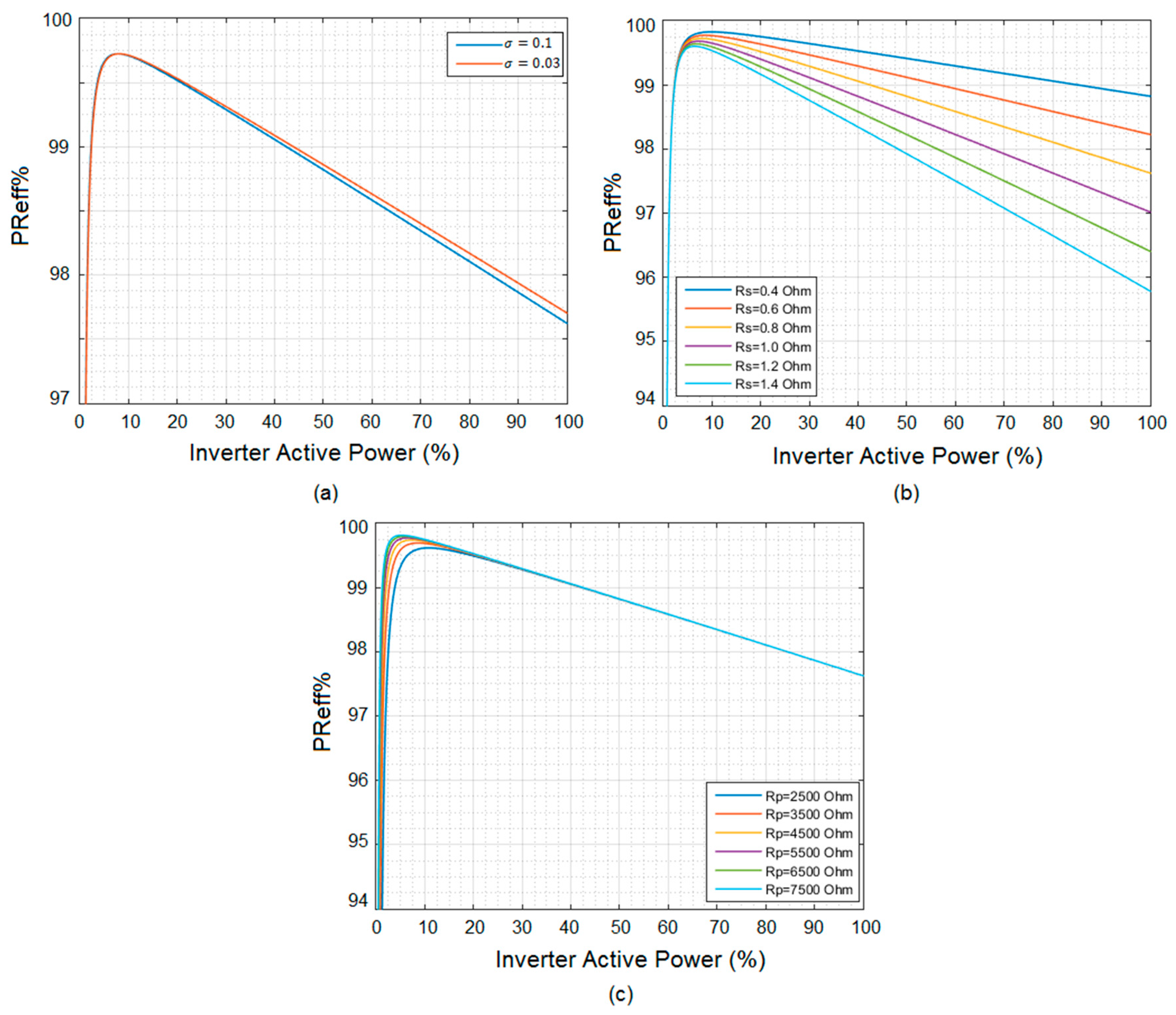
This procedure can be useful for the analysis of the right amount of active power provided for the FFR service during the inertial response after a frequency contingency, or, from the point of view of the active user, it can be used to evaluate the battery power reference for the BMS that ensures the required amount of active power reserve at the bus. In order to provide a clear graphical representation of what is explained above, the quantity is defined as follows, with respect to the theoretical reserve :
Figure 5a shows how varies at different levels of inverter active power production for = 0.1 and = 0.03. As expected, the higher the parameter , the lower the active power reserve efficiency, even if the variation is not very substantial. Figure 5b,c show the dependence of the active power reserve efficiency on series and shunt resistor of the non-ideal inverter model. As for inverter efficiency, the higher the active power operating point of the inverter, the greater the impact of the parameter on the active power reserve efficiency, especially for a very low level of PF. Instead, the effect of a variation of is more visible in the lower part of the inverter operating range, but it does not involve significant impacts at higher operating points. For this reason, it is clear that in the inverter model, a correct experimental extraction of is considerably more important than that of for the effective active power reserve evaluation purpose.
5. Impact of Reactive Power Control on Active Power Reserve Efficiency
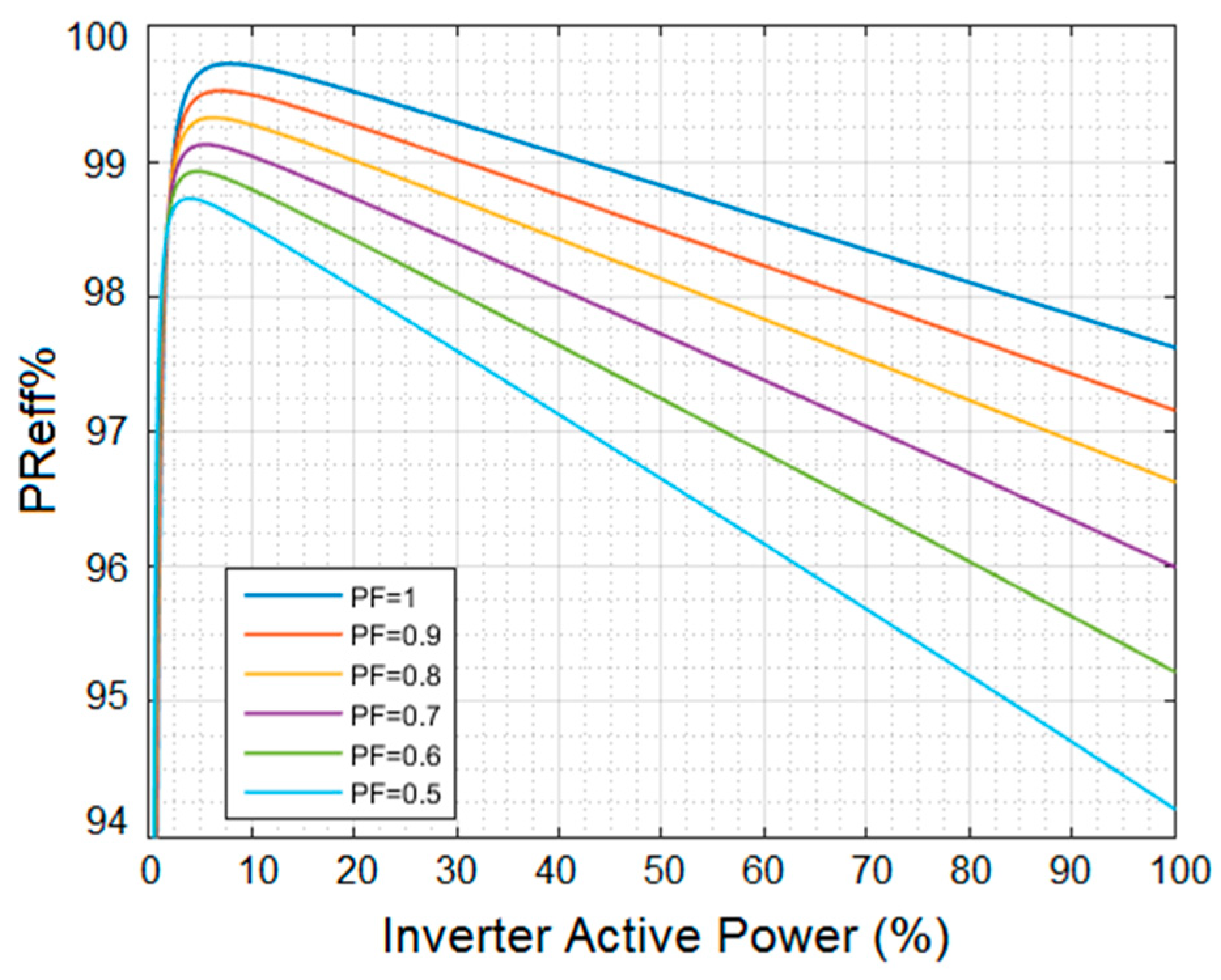
Since the frequency stability is not the only issue for smart grids with high penetration of DG from renewable sources, the PV inverter control for FFR could need to be implemented in parallel with other control strategies [48]. In fact, due to the high injection of active power to the nodes of the grid by the distributed PV plants, some overvoltage problems may occur during the peak hours of the day. For this purpose, the PV inverter is required to absorb reactive power, operating with a PF ≠ 1, in order to mitigate the nodal overvoltage and to comply with the voltage regulation issue. Hence, also a reactive power control needs to be implemented on the inverter control system. Due to these considerations, the behavior of the parameters defined in Section 2 needs to be analyzed in the case of the reactive control operation mode. Considering Equation (4), a variation on the PV inverter reactive power causes a variation on the inverter efficiency [49], also affecting the active power reserve in Equations (13)–(15). Since a 5-kW inverter is analyzed, as anticipated in Section 2, for the sake of simplicity, = 600 V and = 230 V are considered.
In Figure 6, the impact of different levels of PF (from 0.5 to 1) on is depicted. For the purpose of completeness, a low level of PF is also investigated, even though these conditions are not affected by the limitations imposed by the inverter capability curve [50]. As for inverter efficiency, active reserve efficiency decreases when a higher amount of reactive power (i.e., lower power factor) is required.
In order to provide a practical understanding of the impact of reactive power on reserve efficiency, the solar irradiance profiles of both a clear-sky day and a variable day are considered. Starting from the daily global irradiance and temperature of PV modules on a sunny day (Figure 7a) and on a variable day (Figure 7b), the PV output is evaluated and depicted in Figure 7c and in Figure 7d, respectively. Therefore, the active power reserve p.u., for different values of PF, is given as results in Figure 7e (sunny day) and in Figure 7f (variable day), considering = 0.1. A focus on the hours in which the PV output is different from zero is provided.
As expected, the major impact of the reactive power control on the reserve efficiency occurs during the peak hours of the day. Hence, if a certain amount of active power reserve is required at the node, the reactive control strategy adopted could determine extra costs for the active user when the FFR service is provided [51]. In accordance with Equation (4), the reduction of irradiance between 13:30 and 16:30 positively affects reserve efficiency, since the system works on a higher point of the curves depicted in Figure 6, even if the total amount of active power reserve is reduced.
6. Impact of Voltage Control Strategies on Active Power Reserve Efficiency Provided by an LV Grid
In a scenario in which LV active users participate in the FFR service, where the active power reserve provided by LV grid is evaluated at the interconnection node with the higher level of the grid, the impact of the voltage regulation strategies related to the reactive power control becomes crucial. In fact, different strategies for overvoltage mitigation are studied in [52,53,54]:
- N = 0: no regulation (PF = 1);
- N = 1: fixed PF = 0.9;
- N = 2: PF = f(P);
- N = 3: Q = f(V);
- N = 4: PF = f(P,V) (mixed strategy).
For comparison purposes, a new parameter is introduced, similar to the parameters identified in [54,55].
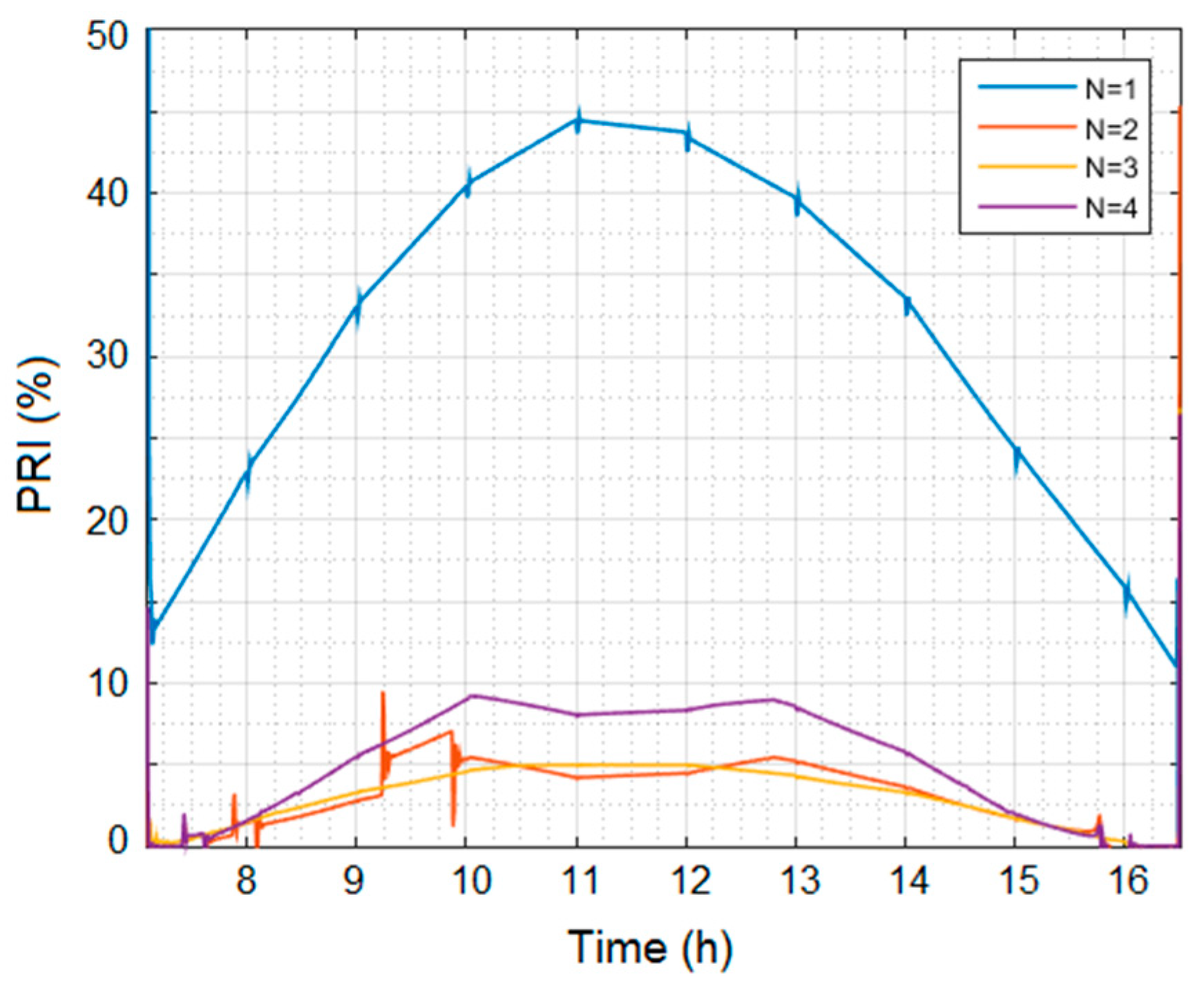
The Power Reserve Index is defined as follows:
Even if this study has a general relevance, a simple eight-bus radial LV grid is considered, in order to better understand the physical meaning of the proposed parameter. Each node from 1 to 8 is equipped with a PV system with BESS, connected to the node by a single-phase inverter; node 0 represents the interconnection point with the upper level of the grid. For the sake of simplicity, the voltage at node 0 is assumed to be fixed at 230 V. The effective active power reserve at node 0 of the grid is evaluated in order to investigate the contribution of grid losses. Electrical lines between two adjacent nodes n and n+1, from node 1 to node 8, are modeled by an R-L series branch with a resistance r = 0.576 Ohm/km and an inductive reactance x = 0.397 Ohm/km. The line 0-1 is differently modeled using different values of resistance and reactance, Rt = 0.0253 Ohm and Xt = 0.025 Ohm, since it represents the connection to the LV busbar of the MV/LV electrical transformer. Since the extension of the LV grid is not very large, the same values of global irradiance and daily temperature are used as inputs for each active node. In addition, each node from 1 to 8 holds an electrical domestic load, connected to the AC bus of the inverter. In this study, typical values of domestic load are used, with a constant power factor PF = 0.9. A minimum irradiance of 400 W/m2 is considered for the activation of active power reserve provision by the BESS.
Power Reserve Index (PRI) defines the difference in the amount of active power reserve at node 0, due to the different reactive power control strategies, as a percentage of the base case (N = 0).
Despite a 24-h simulation being run in MATLAB/Simulink, the results are given for the hours with an effective PV power production, since they are relevant for this analysis. Figure 8 shows the results in the case of no voltage regulation (N = 0).
Notice that the non-perfect correspondence between the blue lines in Figure 7 and Figure 8 is due to the simplifications on and assumed in Section IV. The different impact of inverter losses and grid losses on the active power reserve provided by the LV grid is clear. Starting from this result, the analysis can be conducted on the cases N = 1, 2, 3, 4, in which a voltage regulation strategy is adopted for overvoltage mitigation issues, and the impact of the voltage regulation strategies related to the reactive power control becomes crucial.
Evidently, a lower value of this index represents a better performance in terms of effective active power reserve. The PRI curves are depicted in Figure 9.
As expected, the high amount of reactive power flowing to grid lines, in the case of strategy 1, i.e., fixed PF = 0.9 regulation, determines the highest level of losses through PV inverters and the distribution grid. For this reason, this regulation represents the worst one in terms of reserve efficiency. The performances of the other three regulation strategies are strictly related to the topology of the grid and to the PV inputs. In fact, if PV systems produce high level of active power, strategy three requires the inverter to produce a high level of reactive power, increasing losses and affecting the effective active power reserve at node 0. Otherwise, if nodal overvoltage contingencies become relevant, strategy 2 can determine a high level of PRI. Clearly, line parameters and inverter resistors play a crucial role in power losses. The parameter PRI could be useful for the grid regulator to correctly evaluate the better voltage regulation strategy that guarantees the minimum desired active power reserve at node 0.
7. Conclusions
In this paper, the effective contribution that battery energy storage systems, coupled to photovoltaic systems, can give to the frequency regulation service is explored.
Starting from a simplified inverter model that takes into account its power losses, a mathematical formulation for the evaluation of active power reserve of inverters used for fast frequency response is proposed.
As a result, the effective active power reserve depends on inverter efficiency, percentage of reserve required and operating point of the inverter in the capability curve. This formulation can evaluate the effective amount of active power reserve that the inverter can guarantee during a frequency contingency, starting from the theoretical reserve. Therefore, the impact of reactive power control on this reserve efficiency is analyzed, and the results for both clear-sky and days are given as an example.
The results show a slight dependency of the efficiency on the amount of active power required, while the impact of the reactive power control is considerable, since the reserve efficiency decreases even up to 97% when the inverter operates at PF = 0.9 and near 100% of its rated power.
This result points out the necessity to find the suitable trade-off between reactive power provision for voltage regulation and active power reserve required by the active user for frequency regulation, considering extra power losses in the inverter due to the reactive power production.
Finally, the participation in the fast frequency response of low voltage grid with aggregated photovoltaic generators and storage systems is considered. A new parameter, named Power Reserve Index (PRI), is defined for the comparison of different impact of voltage regulation strategies on the active power reserve efficiency. The results of MATLAB/Simulink simulation are given and discussed, highlighting how the fixed PF strategy represents the worst case in terms of effective active power reserve. In fact, in this case, the parameter PRI varies from 15% to 45% during the regulation time, while it remains below 10% in other strategies.
Since inverter losses represent a cost or missing revenue for a photovoltaic system owner, for prosumers, further works on this topic can be related to the definition of cost functions for provision of ancillary services, taking into account how costs for voltage and frequency regulations are related and how active users can take both of them into account.
Based on the losses and opportunity costs, an application of this work could be the identification of costs and, in turn, the level of bid prices, that the operator of a smart grid needs to consider for the provision of ancillary services to the transmission system operator (TSO) or distribution system operator (DSO) as well as to an aggregator.
Author Contributions
Conceptualization, methodology, writing–review, G.M.T.; validation, formal analysis, writing draft and editing, D.G. All authors have read and agreed to the published version of the manuscript.
Funding
This research was funded by the European Regional Development Funds (P.O. FESR 2014–2020 line 1.1.5) by Regione siciliana (Italy); project name PASCAL and number 084321010342.
Conflicts of Interest
The authors declare no conflict of interest.
References
- European Commission. Annex to the Communication from the Commission to the European Parliament, the European Council, the Council, the European Economic and Social Committee and the Committee of the Regions. In The European Green Deal; European Commission: Brussels, Belgium, 2019. [Google Scholar]
- Gregory, M. Beyond 100% renewable: Policy and practical pathways to 24/7 renewable energy procurement. Electr. J. 2020, 33, 106695. [Google Scholar]
- Choudhary, P.; Srivastava, R.K. Sustainability perspectives- a review for solar photovoltaic trends and growth opportunities. J. Clean. Prod. 2019, 227, 589–612. [Google Scholar] [CrossRef]
- Chiacchio, F.; Famoso, F.; D’Urso, D.; Cedola, L. Performance and Economic Assessment of a Grid-Connected Photovoltaic Power Plant with a Storage System: A Comparison between the North and the South of Italy. Energies 2019, 12, 2356. [Google Scholar] [CrossRef] [Green Version]
- Ciriminna, R.; Albanese, L.; Pecoraino, M.; Meneguzzo, F.; Pagliaro, M. Solar Energy and New Energy Technologies for Mediterranean Countries. Glob. Chall. 2019, 3, 1900016. [Google Scholar] [CrossRef] [PubMed]
- Karimi, M.; Mokhlis, H.; Naidu, K.; Uddin, S.; Bakar, A. Photovoltaic penetration issues and impacts in distribution network–A review. Renew. Sustain. Energy Rev. 2016, 53, 594–605. [Google Scholar] [CrossRef]
- Khan, B.; Tanwar, S. Issues Associated With Microgrid Integration. Adv. Comput. Electr. Eng. 2019, 2019, 252–264. [Google Scholar] [CrossRef] [Green Version]
- Delfanti, M.; Merlo, M.; Monfredini, G.; Cerretti, A.; De Berardinis, E. Voltage regulation issues for smart grid. In Proceedings of the CIGRE 2011 Bologna Symposium-The Electric Power System of the Future: Integrating Supergrids and Microgrids, Paris, France, 13–15 September 2011. [Google Scholar]
- Ruban, N.; Kinshin, A.; Gusev, A. Review of grid codes: Ranges of frequency variation. In Proceedings of the International Youth Scientific Conference “Heat and Mass Transfer in the Thermal Control System of Technical and Technological Energy Equipment” (HMTTSC 2019), Tomsk, Russia, 9 August 2019. [Google Scholar]
- Wooyoung, C. Grid-Connected Inverter to Mitigate Voltage-Based Power Quality Problems; The University of Wisconsin-Madison: Madison, WI, USA, 2019. [Google Scholar]
- Wu, Y.K.; Tang, K.T. Frequency Support by BESS–Review and Analysis. Energy Procedia 2019, 156, 187–191. [Google Scholar] [CrossRef]
- Greenwood, D.; Lim, K.; Patsios, C.; Lyons, P.; Lim, Y.; Taylor, P. Frequency response services designed for energy storage. Appl. Energy 2017, 203, 115–127. [Google Scholar] [CrossRef]
- Meng, L.; Zafar, J.; Khadem, S.K.; Collinson, A.; Murchie, K.C.; Coffele, F.; Burt, G.M. Fast Frequency Response From Energy Storage Systems—A Review of Grid Standards, Projects and Technical Issues. IEEE Trans. Smart Grid 2020, 11, 1566–1581. [Google Scholar] [CrossRef] [Green Version]
- Yagami, M.; Kimura, N.; Tsuchimoto, M.; Tamura, J. Power system transient stability analysis in the case of high-penetration photovoltaics. In Proceedings of the 2013 IEEE Grenoble Conference, Piscataway, NJ, USA, 16–20 June 2013; pp. 1–6. [Google Scholar]
- Dreidy, M.; Mokhlis, H.; Mekhilef, S. Inertia response and frequency control techniques for renewable energy sources: A review. Renew. Sustain. Energy Rev. 2017, 69, 144–155. [Google Scholar] [CrossRef]
- Asmus, P. Microgrids, Virtual Power Plants and Our Distributed Energy Future. Electr. J. 2010, 23, 72–82. [Google Scholar] [CrossRef]
- Marzooghi, H.; Verbic, G.; Hill, D.J. Aggregated demand response modelling for future grid scenarios. Sustain. Energy Grids Netw. 2016, 5, 94–104. [Google Scholar] [CrossRef] [Green Version]
- Cipcigan, L.; Taylor, P.; Lyons, P. A dynamic virtual power station model comprising small-scale energy zones. Int. J. Renew. Energy Technol. 2009, 1, 173. [Google Scholar] [CrossRef]
- Chen, S.; Zhang, T.; Gooi, H.B.; Masiello, R.D.; Katzenstein, W. Penetration Rate and Effectiveness Studies of Aggregated BESS for Frequency Regulation. IEEE Trans. Smart Grid 2015, 7, 1. [Google Scholar] [CrossRef]
- Tang, W.J.; Yang, H.T. Optimal Operation and Bidding Strategy of a Virtual Power Plant Integrated With Energy Storage Systems and Elasticity Demand Response. IEEE Access 2019, 7, 79798–79809. [Google Scholar] [CrossRef]
- Nosratabadi, S.M.; Hooshmand, R.A.; Gholipour, E. A comprehensive review on microgrid and virtual power plant concepts employed for distributed energy resources scheduling in power systems. Renew. Sustain. Energy Rev. 2017, 67, 341–363. [Google Scholar] [CrossRef]
- Comodi, G.; Giantomassi, A.; Severini, M.; Squartini, S.; Ferracuti, F.; Fonti, A.; Cesarini, D.N.; Morodo, M.; Polonara, F. Multi-apartment residential microgrid with electrical and thermal storage devices: Experimental analysis and simulation of energy management strategies. Appl. Energy 2015, 137, 854–866. [Google Scholar] [CrossRef]
- Samarakoon, K.; Ekanayake, J.; Jenkins, N. Investigation of Domestic Load Control to Provide Primary Frequency Response Using Smart Meters. IEEE Trans. Smart Grid 2011, 3, 282–292. [Google Scholar] [CrossRef]
- Rezkalla, M.M.; Zecchino, A.; Pertl, M.; Marinelli, M. Grid frequency support by single-phase electric vehicles employing an innovative virtual inertia controller. In Proceedings of the 2016 51st International Universities Power Engineering Conference (UPEC), Piscataway, NJ, USA, 6–9 September 2016; pp. 1–6. [Google Scholar]
- Rezkalla, M.M.; Zecchino, A.; Martinenas, S.; Prostejovsky, A.; Marinelli, M. Comparison between synthetic inertia and fast frequency containment control based on single phase EVs in a microgrid. Appl. Energy 2018, 210, 764–775. [Google Scholar] [CrossRef] [Green Version]
- Marconato, R. Electric Power Systems; CEI: Milan, Italy, 2002. [Google Scholar]
- Italian Standard, CEI. Reference Technical Rules for the Connection of Active and Passive Users to the LV Electrical Utilities; CEI: Milan, Italy, 2019. [Google Scholar]
- Italian Standard, CEI. Reference Technical Rules for the Connection of Active and Passive Consumers to the HV and MV Electrical Networks of Distribution Company; CEI: Milan, Italy, 2019. [Google Scholar]
- Tina, G.M.; Celsa, G. Active and reactive power regulation in grid-connected PV systems. In Proceedings of the 2015 50th International Universities Power Engineering Conference (UPEC), Piscataway, NJ, USA, 1–4 September 2015; pp. 1–6. [Google Scholar]
- Tina, G.M. Simulation Model of Photovoltaic and Photovoltaic/Thermal Module/String under Nonuniform Distribution of Irradiance and Temperature. J. Sol. Energy Eng. 2016, 139, 021013. [Google Scholar] [CrossRef]
- Yao, L.W.; Aziz, J.A.; Kong, P.Y.; Idris, N.R.N.; Aziz, M.J.A. Modeling of lithium-ion battery using MATLAB/simulink. In Proceedings of the IECON 2013-39th Annual Conference of the IEEE Industrial Electronics Society, Piscataway, NJ, USA, 10–13 November 2013; pp. 1729–1734. [Google Scholar]
- Chen, M.; Rincon-Mora, G. Accurate Electrical Battery Model Capable of Predicting Runtime and I–V Performance. IEEE Trans. Energy Convers. 2006, 21, 504–511. [Google Scholar] [CrossRef]
- Wen, J.; Yu, Y.; Chen, C. A Review on Lithium-Ion Batteries Safety Issues: Existing Problems and Possible Solutions. Mater. Express 2012, 2, 197–212. [Google Scholar] [CrossRef]
- Millner, A. Modeling Lithium Ion battery degradation in electric vehicles. In Proceedings of the 2010 IEEE Conference on Innovative Technologies for an Efficient and Reliable Electricity Supply, Piscataway, NJ, USA, 27–29 October 2010; pp. 349–356. [Google Scholar]
- Tina, G.M.; Celsa, G. A Matlab/Simulink model of a grid connected single-phase inverter. In Proceedings of the 2015 50th International Universities Power Engineering Conference (UPEC), Stroke-on-Trent, UK, 9 April 2015; pp. 1–6. [Google Scholar] [CrossRef]
- Chivelet, N.M.; Chenlo, F.; Alonso, M.C. Modelado y Fiabilidad de Inversores para Instalaciones Fotovoltaicas Autónomas a Partir de Medidas com cargas Resistivas y Reactivas. In Proceedings of the VII Congreso Ibérico de Energia Solar, Vigo, Spain, 17–21 June 1994. [Google Scholar]
- Luis Dávila, G. Modelado para la Simulación, el Diseño y la Validación de Inversores Fotovoltaicos Conectados a la Red Eléctrica. Ph.D. Thesis, Universidad Nacional de Educación a Distancia (España), Madrid, Spain, 2011. [Google Scholar]
- Rahmann, C.; Castillo, A. Fast Frequency Response Capability of Photovoltaic Power Plants: The Necessity of New Grid Requirements and Definitions. Energies 2014, 7, 6306–6322. [Google Scholar] [CrossRef]
- Zarina, P.; Mishra, S.; Sekhar, P.; Mishra, S. Photovoltaic system based transient mitigation and frequency regulation. In Proceedings of the 2012 Annual IEEE India Conference (INDICON), Piscataway, NJ, USA, 7–9 December 2012; pp. 1245–1249. [Google Scholar]
- Zarina, P.P.; Mishra, S.; Sekhar, P.C. Deriving inertial response from a non-inertial PV system for frequency regulation. In Proceedings of the 2012 IEEE International Conference on Power Electronics, Drives and Energy Systems (PEDES), Piscataway, NJ, USA, 16–19 September 2012; pp. 1–5. [Google Scholar]
- Hoke, A.F.; Muljadi, E.; Maksimović, D.; Anderson, H. Real-time photovoltaic plant maximum power point estimation for use in grid frequency stabilization. In Proceedings of the 2015 IEEE 16th Workshop on Control and Modeling for Power Electronics (COMPEL), Vancouver, BC, Canada, 12–15 July 2015. [Google Scholar] [CrossRef]
- Hoke, A.F.; Shirazi, M.; Chakraborty, S.; Muljadi, E.; Maksimovic, D. Rapid Active Power Control of Photovoltaic Systems for Grid Frequency Support. IEEE J. Emerg. Sel. Top. Power Electron. 2017, 5, 1154–1163. [Google Scholar] [CrossRef]
- Villalva, M.; Gazoli, J.R.; Filho, E. Comprehensive Approach to Modeling and Simulation of Photovoltaic Arrays. IEEE Trans. Power Electron. 2009, 24, 1198–1208. [Google Scholar] [CrossRef]
- Lian, B.; Sims, A.; Yu, D.; Wang, C.; Dunn, R.W. Optimizing LiFePO4 Battery Energy Storage Systems for Frequency Response in the UK System. IEEE Trans. Sustain. Energy 2016, 8, 385–394. [Google Scholar] [CrossRef]
- Zhai, Q.; Meng, K.; Dong, Z.Y.; Ma, J. Modeling and Analysis of Lithium Battery Operations in Spot and Frequency Regulation Service Markets in Australia Electricity Market. IEEE Trans. Ind. Inform. 2017, 13, 2576–2586. [Google Scholar] [CrossRef]
- Shoubaki, E.; Essakiappan, S.; Manjrekar, M.; Enslin, J. Synthetic inertia for BESS integrated on the DC-link of grid-tied PV inverters. In Proceedings of the 2017 IEEE 8th International Symposium on Power Electronics for Distributed Generation Systems (PEDG), Florianopolis, Brazil, 17–20 April 2017; Volume 32, pp. 1–5. [Google Scholar] [CrossRef]
- Xu, B.; Oudalov, A.; Poland, J.; Ulbig, A.; Andersson, G. BESS Control Strategies for Participating in Grid Frequency Regulation. IFAC Proc. Vol. 2014, 47, 4024–4029. [Google Scholar] [CrossRef] [Green Version]
- Adhikari, S.; Li, F. Coordinated V-f and P-Q Control of Solar Photovoltaic Generators with MPPT and Battery Storage in Microgrids. IEEE Trans. Smart Grid 2014, 5, 1270–1281. [Google Scholar] [CrossRef]
- Demirok, E.; Sera, D.; Teodorescu, R. Investigation of extra power loss sharing among photovoltaic inverters caused by reactive power management in distribution networks. In Proceedings of the 2014 IEEE Energy Conversion Congress and Exposition (ECCE), Pittsburgh, PA, USA, 14–18 September 2014. [Google Scholar] [CrossRef]
- Cabrera-Tobar, A.; Bullich-Massagué, E.; Aragüés-Peñalba, M.; Gomis-Bellmunt, O. Capability curve analysis of photovoltaic generation systems. Sol. Energy 2016, 140, 255–264. [Google Scholar] [CrossRef] [Green Version]
- Braun, M. Reactive power supplied by pv inverters–cost-benefit-analysis. In Proceedings of the 22nd European Photovoltaic Solar Energy Conference and Exhibition, Milan, Italy, 3–7 September 2007. [Google Scholar]
- Demirok, E.; González, P.C.; Frederiksen, K.H.B.; Sera, D.; Rodriguez, P.; Teodorescu, R. Local Reactive Power Control Methods for Overvoltage Prevention of Distributed Solar Inverters in Low-Voltage Grids. IEEE J. Photovolt. 2011, 1, 174–182. [Google Scholar] [CrossRef]
- Momeneh, A.; Castilla, M.; Velasco, M.; Miret, J.; Martí, P.; Velasco, M. Comparative study of reactive power control methods for photovoltaic inverters in low-voltage grids. IET Renew. Power Gener. 2016, 10, 310–318. [Google Scholar] [CrossRef] [Green Version]
- Garozzo, D.; Tina, G.; Sera, D. Comparison of the reactive control strategies in LV network with PV generation and storage. Therm. Sci. 2018, 22, 22. [Google Scholar] [CrossRef] [Green Version]
- Ishaq, J.; Fawzy, Y.T.; Buelo, T.; Engel, B.; Witzmann, R. Voltage control strategies of low voltage distribution grids using photovoltaic systems. In Proceedings of the 2016 IEEE International Energy Conference (ENERGYCON), Piscataway, NJ, USA, 4–8 April 2016; pp. 1–7. [Google Scholar]
Figure 1.
Voltage regulation curves in Italian Standards: PF = f(P) (a) and Q = f(V) (b).

Figure 2.
Frequency regulation curves in Italian Standards for unidirectional (a) and bidirectional (b) converters.
Figure 2.
Frequency regulation curves in Italian Standards for unidirectional (a) and bidirectional (b) converters.
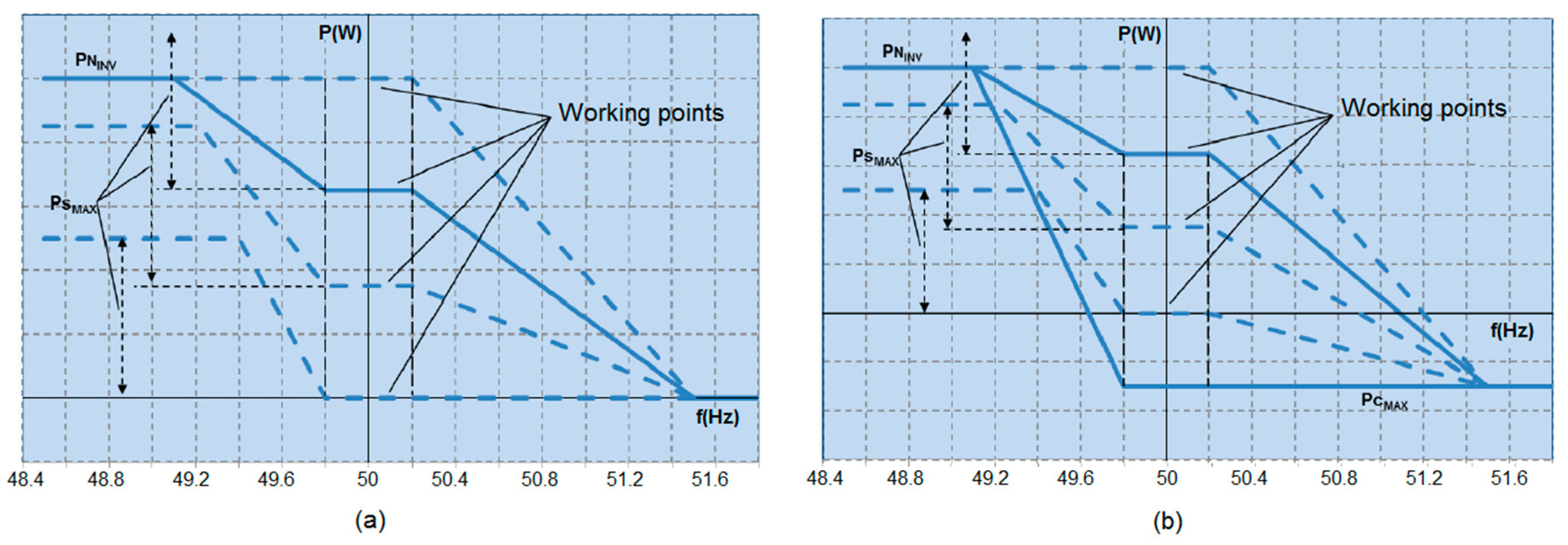
Figure 3.
Photovoltaic + battery energy storage system (PV+BESS) node with non-ideal inverter.

Figure 4.
De-loaded operation mode on photovoltaic P–V curve to provide power reserve.
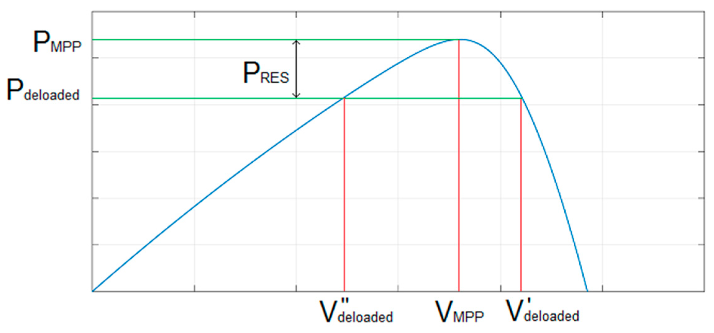
Figure 5.
Dependence of the effective active power reserve on the required reserve parameter (a), series resistance (b) and shunt resistance (c).
Figure 5.
Dependence of the effective active power reserve on the required reserve parameter (a), series resistance (b) and shunt resistance (c).

Figure 6.
Impact of the reactive power on the reserve efficiency at different power factors.

Figure 7.
Solar irradiance and temperature of PV modules (a,b), PV active power output (c,d) and corresponding power reserve p.u. at different power factors (PFs) (e,f) on a clear-sky day (left) and a variable day (right).
Figure 7.
Solar irradiance and temperature of PV modules (a,b), PV active power output (c,d) and corresponding power reserve p.u. at different power factors (PFs) (e,f) on a clear-sky day (left) and a variable day (right).
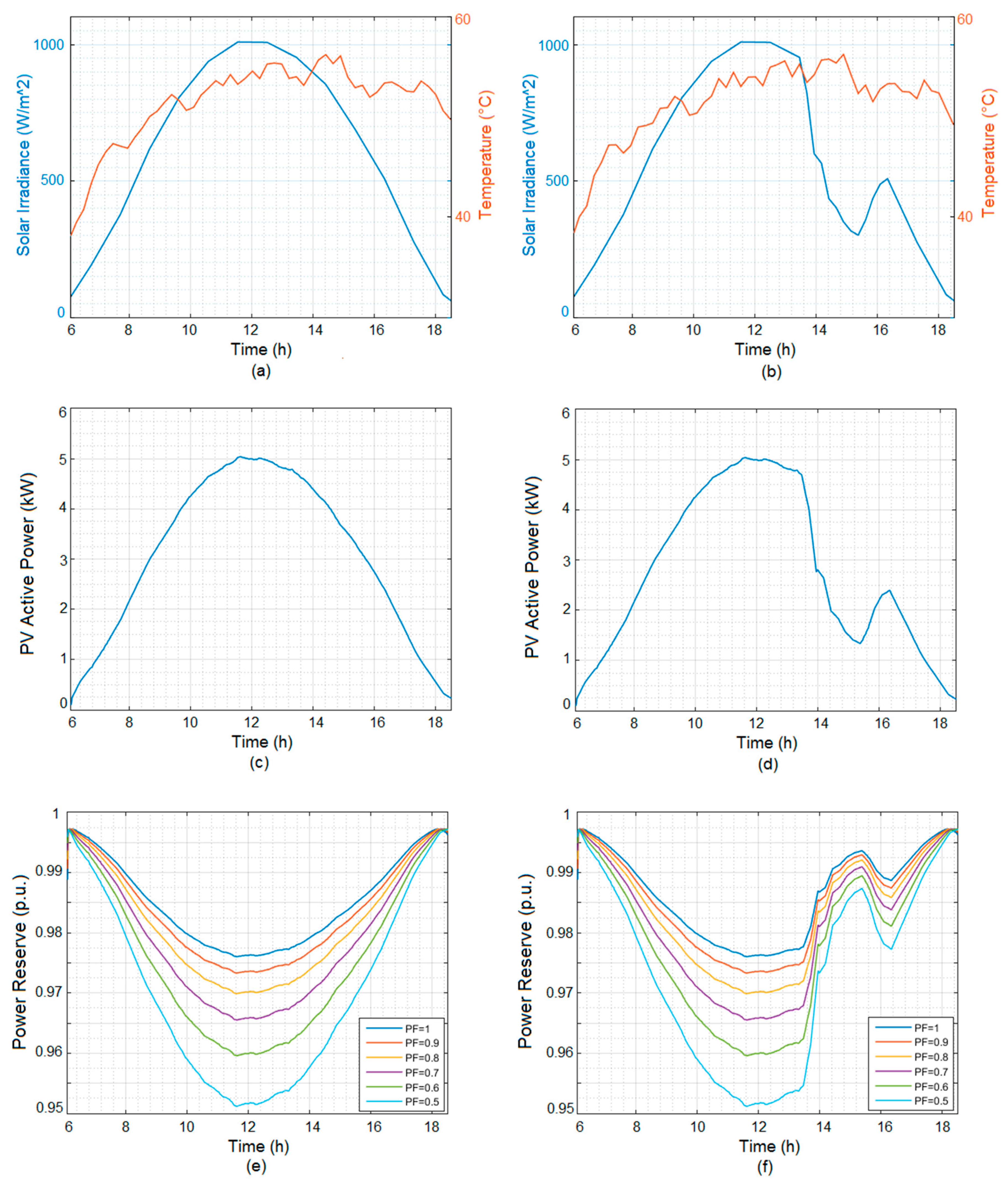
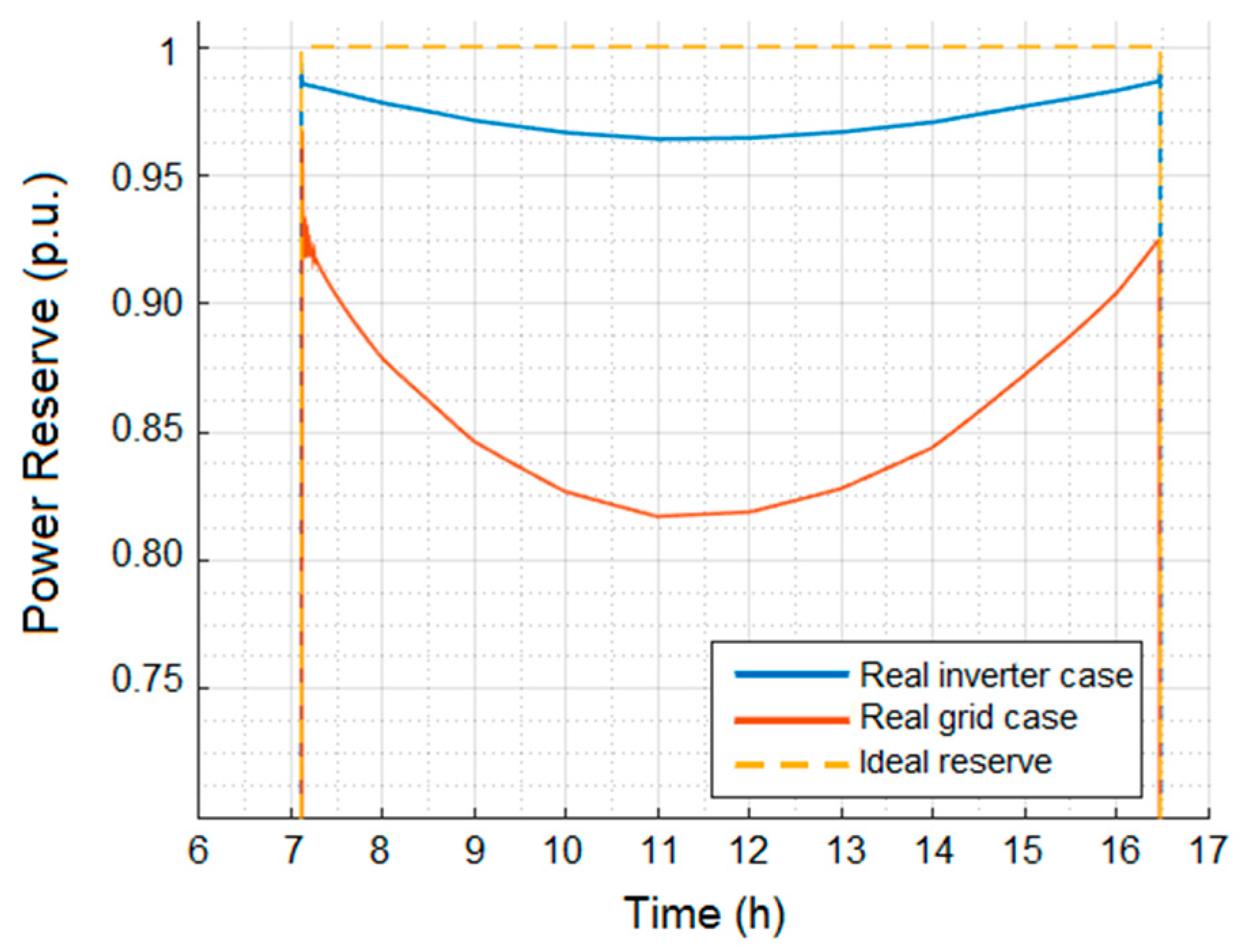
Figure 8.
Effective active power reserve at node 0 in the case of no voltage regulation (N = 0).

Figure 9.
Power Reserve Index during the voltage regulation hours considering different voltage regulation strategies (N = 1:4).
Figure 9.
Power Reserve Index during the voltage regulation hours considering different voltage regulation strategies (N = 1:4).

© 2020 by the authors. Licensee MDPI, Basel, Switzerland. This article is an open access article distributed under the terms and conditions of the Creative Commons Attribution (CC BY) license (http://creativecommons.org/licenses/by/4.0/).
Share and Cite
MDPI and ACS Style
Garozzo, D.; Tina, G.M. Evaluation of the Effective Active Power Reserve for Fast Frequency Response of PV with BESS Inverters Considering Reactive Power Control. Energies 2020, 13, 3437. https://doi.org/10.3390/en13133437
AMA Style
Garozzo D, Tina GM. Evaluation of the Effective Active Power Reserve for Fast Frequency Response of PV with BESS Inverters Considering Reactive Power Control. Energies. 2020; 13(13):3437. https://doi.org/10.3390/en13133437
Chicago/Turabian StyleGarozzo, Dario, and Giuseppe Marco Tina. 2020. "Evaluation of the Effective Active Power Reserve for Fast Frequency Response of PV with BESS Inverters Considering Reactive Power Control" Energies 13, no. 13: 3437. https://doi.org/10.3390/en13133437
Note that from the first issue of 2016, this journal uses article numbers instead of page numbers. See further details here.