Performance Assessment of an Energy Management System for a Home Microgrid with PV Generation


Abstract
:
1. Introduction
- This paper attempts to fill the gap in the literature by employing data for energy consumption and generation collected from real prosumers across the UK.
- It studies the importance of designing an HEMS which is able to respond quickly to changes in the system by operating with a short sample time (in this case two minutes), and analyses the resulting impact on the annual energy costs and the ratio of annual lost PV generated energy to the utility.
- It studies the performance of a HEMS which takes its own decisions locally while minimizing its dependence on external forecasting technologies (and complex communication infrastructures).
- It summarizes the requirements and challenges for HEMS and their impact on household energy costs; this can be considered an aid to selecting an appropriate controller for each PV-battery system.
- It studies the effect of forecasting errors, sample time resolution, tariff policies, the battery capacity and/or PV system on the performance of the MPC.
2. Real-Time Controller-Based Energy Management System
2.1. HBSS Discharging Mode
- If the household is drawing power from the supply utility at the point of grid connection, the HBSS tries to minimize the energy purchased by discharging the HBSS.
- If the household is drawing power from the supply utility and the power drawn is greater than the maximum discharge power of the HBSS, the HBSS will discharge at its maximum power and the remaining power will be purchased from the utility.
- If the household is drawing power from the supply utility and the HBSS state of charge (SOC) reaches its minimum value, the HBSS will cease discharging.
2.2. HBSS Charging Mode
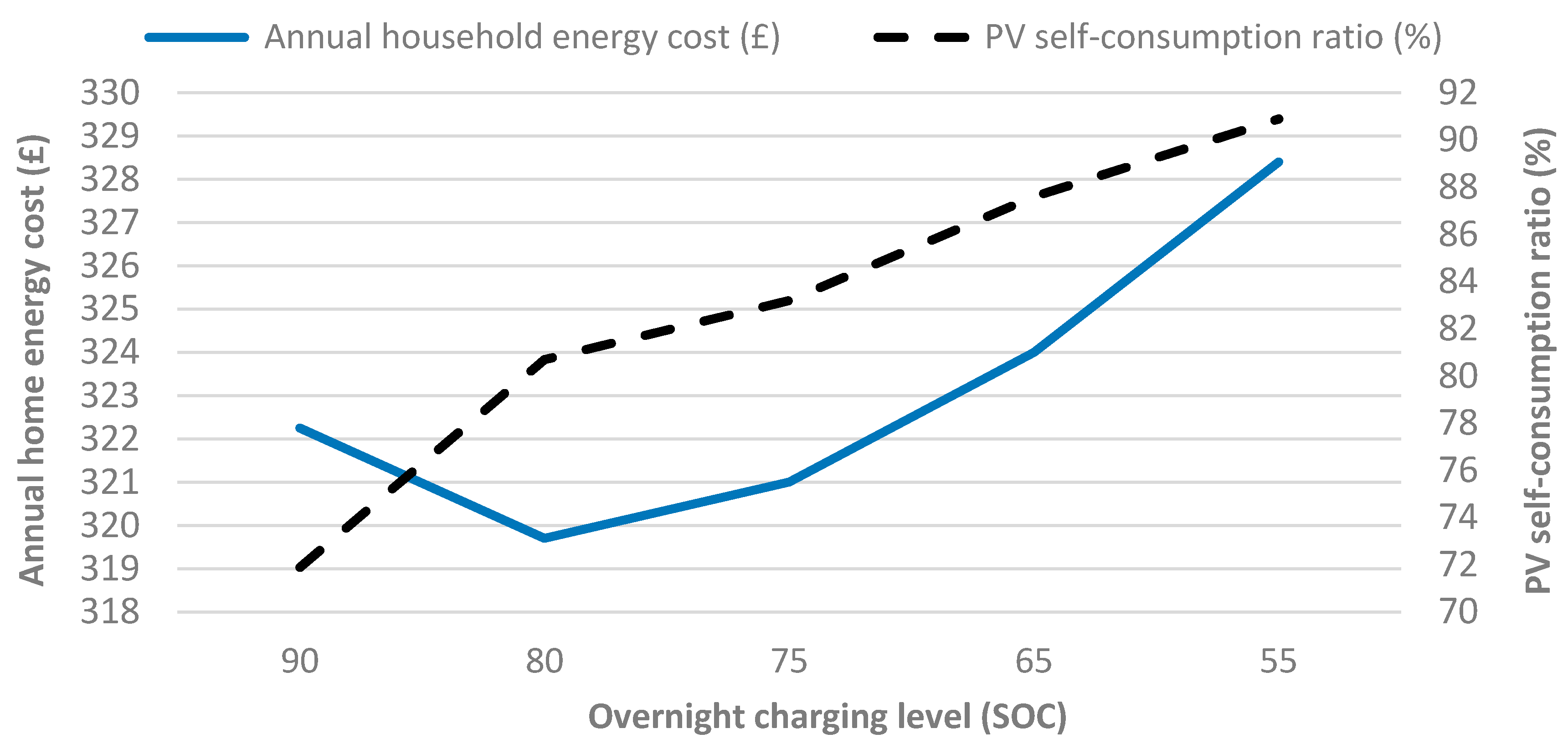
2.2.1. Adjustment of the Low Tariff (Overnight) Charging Level
- Yearly Optimized Overnight Charging: The battery is charged overnight to an optimized pre-set level (fixed throughout the year) depending on the battery capacity and the PV system size. This approach should yield better results than Constant Full Overnight Charging, as the battery is not always fully charged overnight and can be charged by any surplus PV generation.
- Seasonal Optimized Overnight Charging: Each season, the overnight charging level is adjusted to a different value. This value is selected based on the season and the PV and battery sizes. It is assumed that the HBSS contains a calendar timer to adjust the charging level at the beginning of each season. For example, for summer, the lowest charging level will be selected so that the HBSS is able to capture all excess PV generation during the next day.
- Previous Day Modification: The overnight charging level is adjusted based on the charging pattern for the previous day. For example, the overnight charging level increases by 10% for the current day if peak tariff energy was purchased during the previous day. The overnight charge level for the current day decreases by 10% if surplus PV energy was exported to the power grid the day before.
- Weather prediction for the next day(i.e., next day PV generation forecasting): Weather forecast data for the next day is used to adjust the overnight charging level of the battery which leaves capacity for the battery to be charged by the expected surplus PV generation the next day. Internet access is needed to download the meteorological forecast data for the next day and a PV forecasting model is needed to forecast the PV generation pattern. The weather forecast data is used to generate a forecasted PV generation pattern for the next day and then (1) is used to adjust the overnight charging level.
2.2.2. Charging Using Excess PV Energy
- If the home is feeding power to the utility, the HBSS charges to store the surplus energy.
- If the home is feeding power to the utility and this is greater than the HBSS maximum charging power, the HBSS will charge at its maximum charging power and the remaining power will be fed into the utility.
- If the home is feeding power to the utility and HBSS SOC reaches its maximum value, the HBSS will stop charging.
3. Model Predictive Control-Based Energy Management System
3.1. Formulation of the Optimization Problem and Constraints
3.2. Forecasting Methods
- the previous day’s load profile (L-PD).
- the previous week, same day load profile (L-PWSD).
- the average load profile of the previous week (L-AV).
- one of the load demand forecasting techniques (L-FP) of [34], such as ANN, auto regression integrated moving average (ARIMA)+ANN, adaptive neuro-fuzzy inference system (ANFIS) which show better results for demand forecasting.
- the previous day’s PV generation profile (PV-PD).
- the average PV generation profile of the previous week (PV-AV).
- the next day’s weather prediction data + PV forecasting model to determine accurately the forecasted PV pattern for the next day (PV-FP) [15]. The next day’s forecasted PV profile can be received and updated every sample time. This forecasting method needs continuous internet access. This service is available from the utility company or a retail agent for an extra cost.
4. Case Study
5. Performance Indicators
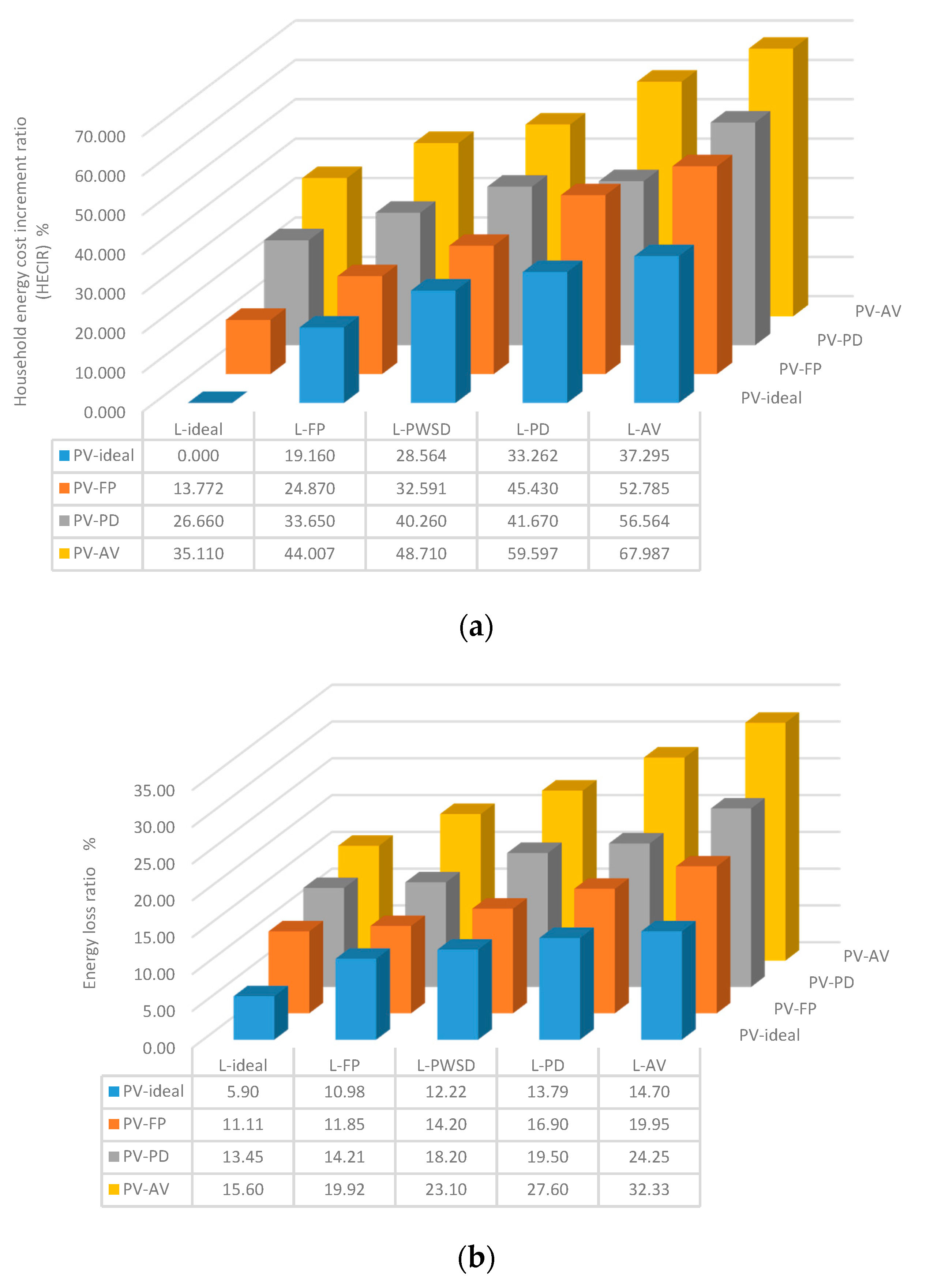
- Household energy cost increment ratio (HECIR): The HECIR is the ratio of the actual household energy costs to the household energy costs that would be achieved in the ideal case, (16). If the value of the HECIR is 0, this means the system has ideal performance. As the value of the HECIR increases, this will indicate higher energy costs and lower system performance. The actual household energy costs are calculated using Equations (2)–(4). The ideal case for the household energy cost when using RTC will occur when the overnight charging level is determined accurately with zero forecasting error for PV generation. The ideal case for the household energy cost when using the MPC will occur when there is zero forecasting error for PV generation and load demand, and the lowest sample time of two minutes is used for the MPC implementation. For both of these cases the actual load/PV data is used for the forecast (i.e., there is an “ideal” forecast).
- PV self-consumption ratio (PVSCR): This metric is used to calculate the quantity of the PV energy used in the home either directly or via the HBSS. The PVSCR is calculated by dividing the PV energy used in the house by the total PV energy generated, (17). A value of 100% indicates all the PV energy generated is used in the house and there is no export to the supply utility.
- Energy lost ratio (ELR): The ELR is determined by dividing all the “lost energy” by the all PV energy generated (18). The “lost energy” is the exported energy to the supply utility because of (a) errors in forecasting, (b) larger sample times which lead to inaccurate power settings for the HBSS, (c) periods when the HBSS is fully charged and no further surplus energy can be stored. Ideally this lost energy should be stored in the battery to be used at peak tariff periods. This ratio is used to assess the performance of the MPC operation, with 0% meaning no lost energy. As the value of the ELR increases, more lost energy will accrue, leading to higher energy charges. The ELR index incorporates both the (unwanted) export resulting from inaccurate HBSS reference settings and from any surplus energy from the PV generation system: note that the complement of the PVSRC only quantifies the exported energy from the PV generation system during the day.
6. RTC-Based HEMS—Results
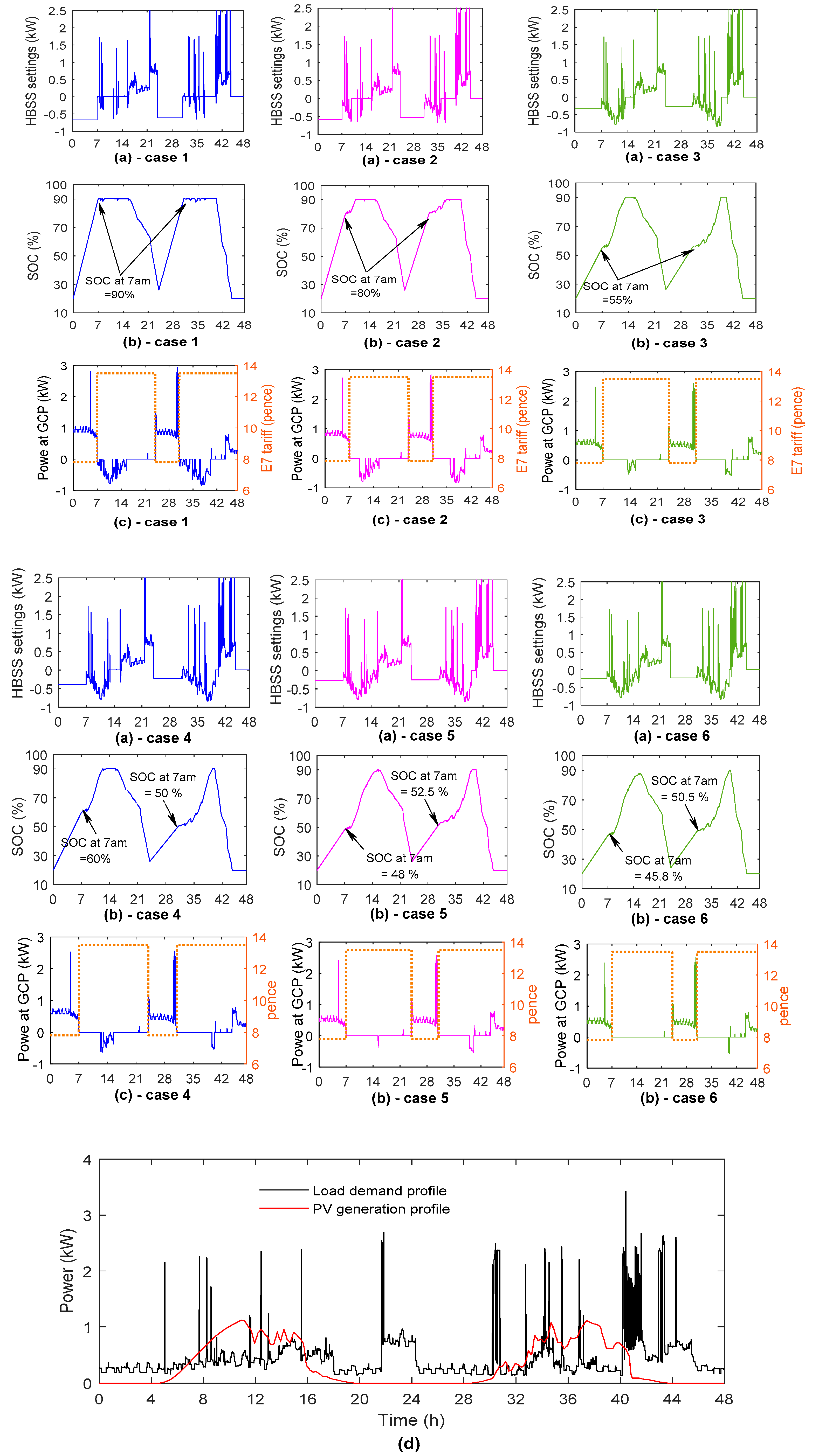
6.1. Simulation Results for the RTC-Based HEMS for Two Days
6.2. Annual Performance Analysis for the RTC-Based HEMS
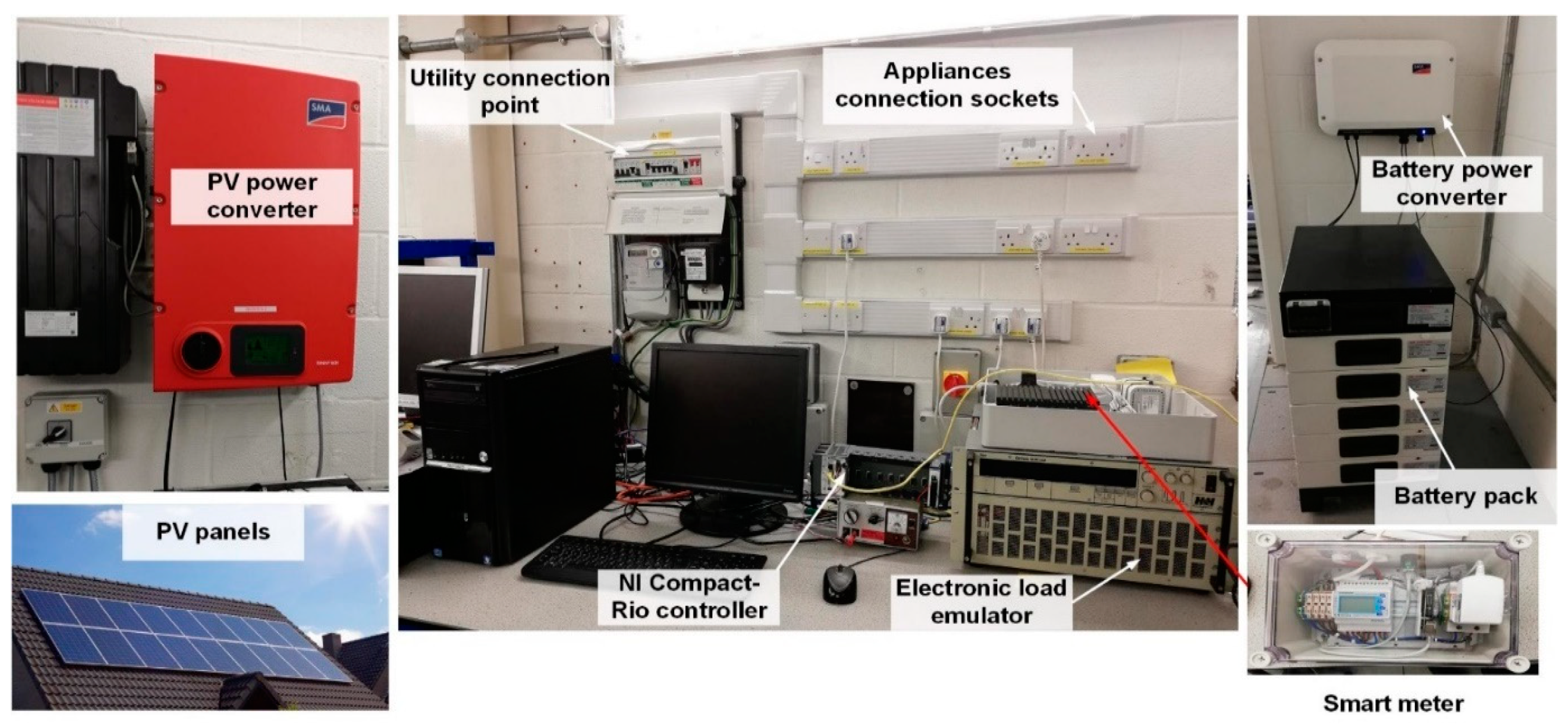
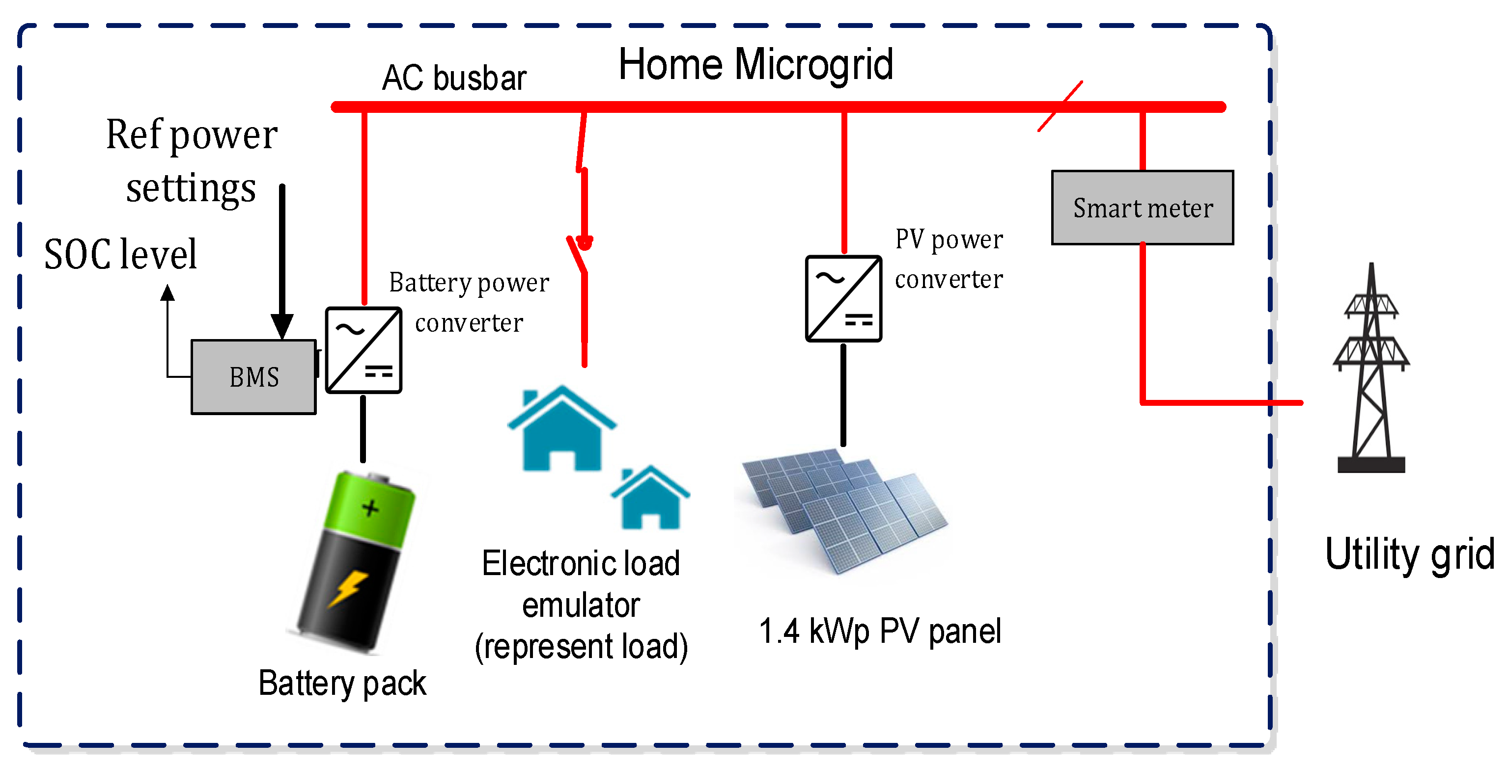
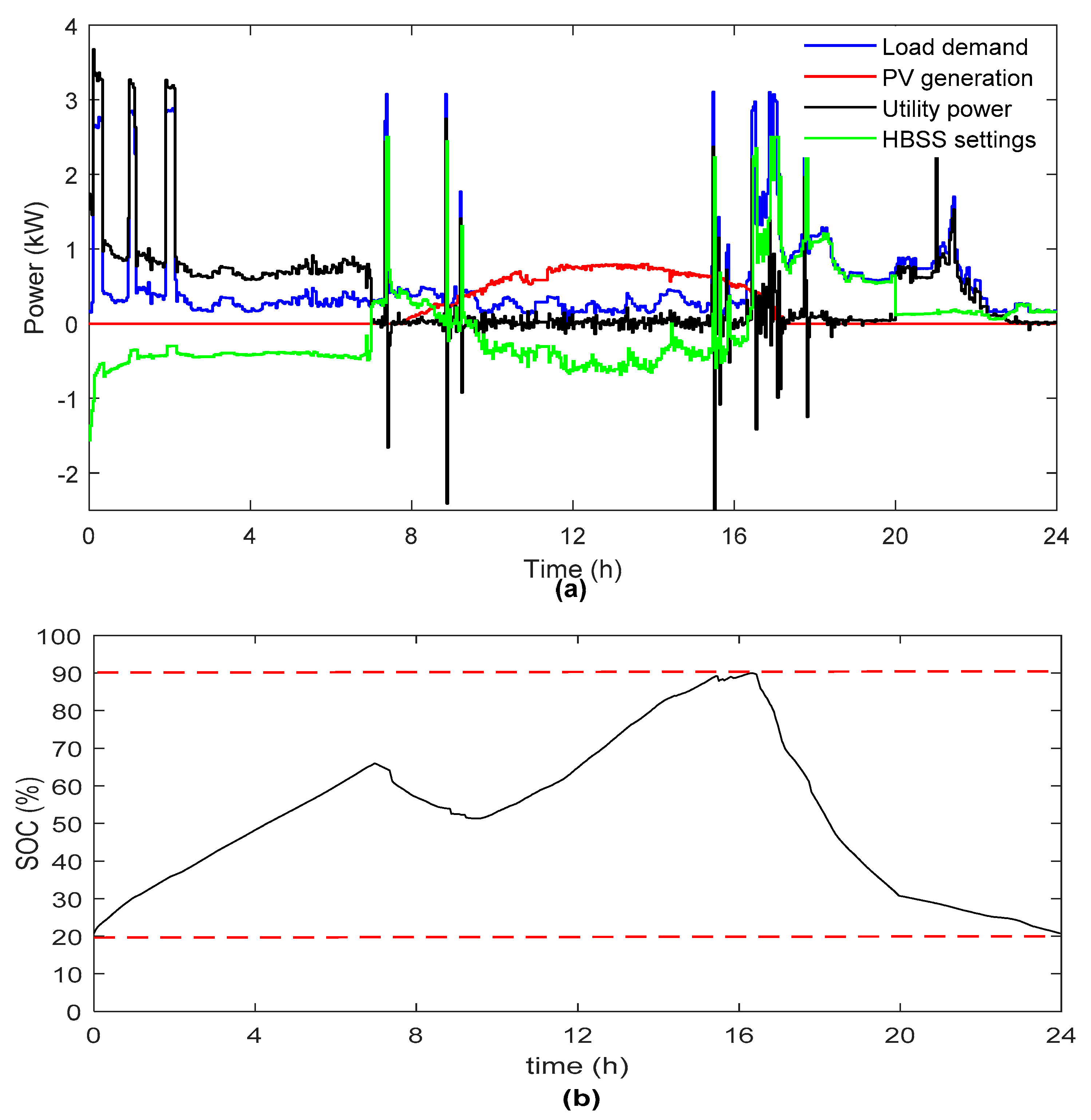
7. MPC Based HEMS—Experimental Results
- 1.4 kWp PV system with a 3.68 kW SMA PV inverter [47]. The PV solar panels are located on the rooftop of the FlexElec laboratory.
- ZSAC Electronic AC load emulator, 5.6 kW [48]: the programmable load emulator receives the digital load demand profiles and creates a real current/power profile drawn from one of the appliance sockets in the SHR. LabVIEW software and a NI CRio FPGA system [49] extract the numerical load values from the database and send them to the programmable load emulator as a reference value.
- Smart meter: a three-phase smart meter used to measure PV generation, load demand, and the power imported/exported by the house from/to the supply utility. The smart meter uses a two minute sample time [50].
- PC: Core i3-7100 CPU, 3.91 GHz PC: the PC is used to run the HEMS.
- Raspberry Pi: used as a Modbus communication interface between the smart meter and the battery management software on the PC. It is also used as a communication interface between the battery management software on the PC and the battery power converter to send the optimal power settings to the SMA converter of the HBSS, and read the actual SOC of the battery.
- Software used: (a) MATLAB—to execute the optimization algorithm and perform the forecasting process, and (b) LABVIEW software package—to control the programmable load emulator.
8. Performance Analysis for the MPC-Based HEMS
8.1. Sample Time Resolution
8.2. The Effect of Forecasting Errors
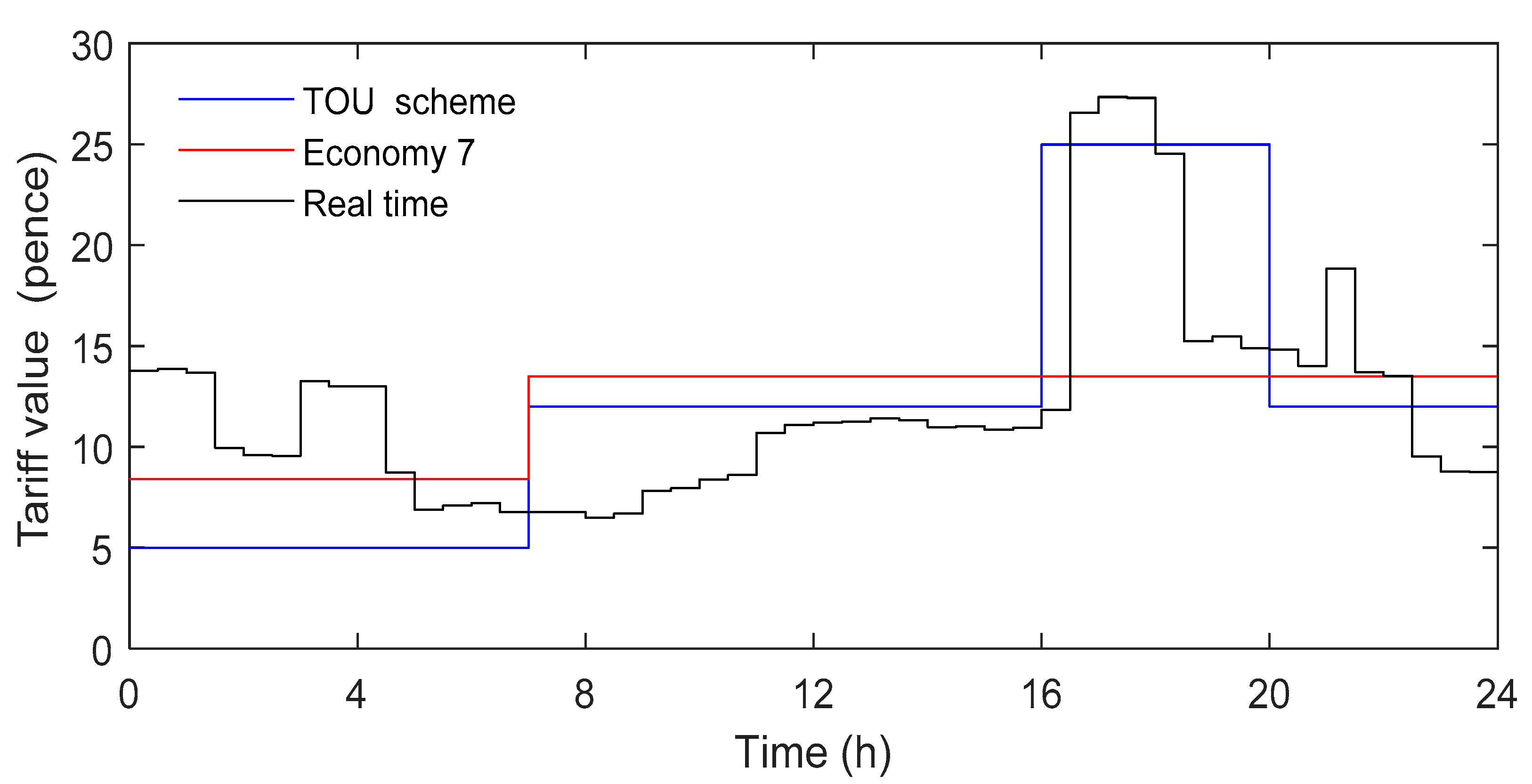
8.3. The Effect of Changing Tariff
8.4. Variation of HBSS Capacity
8.5. Varying PV System Size
9. Conclusions
Author Contributions
Funding
Conflicts of Interest
Appendix A
References
- Chandra, L.; Chanana, S. Energy Management of Smart Homes with Energy Storage, Rooftop PV and Electric Vehicle. In Proceedings of the 2018 IEEE International Students’ Conference on Electrical, Electronics and Computer Science (SCEECS), Bhopal, India, 24–25 February 2018; 2018; pp. 1–6. [Google Scholar]
- Mehdi, L.; Ouallou, Y.; Mohamed, O.; Hayar, A. New Smart Home’s Energy Management System Design and Implementation for Frugal Smart Cities. In Proceedings of the 2018 International Conference on Selected Topics in Mobile and Wireless Networking (MoWNeT), Tangier, Morocco, 20–22 June 2018; 2018; pp. 149–153. [Google Scholar]
- Lebrón, C.; Andrade, F.; O’Neill, E.; Irizarry, A. An intelligent Battery management system for home Microgrids. In Proceedings of the 2016 IEEE Power & Energy Society Innovative Smart Grid Technologies Conference (ISGT), Minneapolis, MN, USA, 6–9 September 2016; 2016; pp. 1–5. [Google Scholar]
- Terlouw, T.; AlSkaif, T.; Bauer, C.; van Sark, W. Multi-objective optimization of energy arbitrage in community energy storage systems using different battery technologies. Appl. Energy 2019, 239, 356–372. [Google Scholar] [CrossRef]
- Van Der Stelt, S.; AlSkaif, T.; van Sark, W. Techno-economic analysis of household and community energy storage for residential prosumers with smart appliances. Appl. Energy 2018, 209, 266–276. [Google Scholar] [CrossRef]
- Sun, C.; Sun, F.; Moura, S.J. Nonlinear predictive energy management of residential buildings with photovoltaics & batteries. J. Power Sources 2016, 325, 723–731. [Google Scholar]
- Wang, G.; Zhang, Q.; Li, H.; McLellan, B.C.; Chen, S.; Li, Y.; Tian, Y. Study on the promotion impact of demand response on distributed PV penetration by using non-cooperative game theoretical analysis. Appl. Energy 2017, 185, 1869–1878. [Google Scholar] [CrossRef] [Green Version]
- Muratori, M.; Rizzoni, G. Residential demand response: Dynamic energy management and time-varying electricity pricing. IEEE Trans. Power Syst. 2015, 31, 1108–1117. [Google Scholar] [CrossRef]
- Erdinc, O. Economic impacts of small-scale own generating and storage units, and electric vehicles under different demand response strategies for smart households. Appl. Energy 2014, 126, 142–150. [Google Scholar] [CrossRef]
- Erdinc, O.; Paterakis, N.G.; Mendes, T.D.; Bakirtzis, A.G.; Catalão, J.P. Smart household operation considering bi-directional EV and ESS utilization by real-time pricing-based DR. IEEE Trans. Smart Grid 2014, 6, 1281–1291. [Google Scholar] [CrossRef]
- Paterakis, N.G.; Taşcıkaraoğlu, A.; Erdinc, O.; Bakirtzis, A.G.; Catalao, J.P. Assessment of demand-response-driven load pattern elasticity using a combined approach for smart households. IEEE Trans. Ind. Inform. 2016, 12, 1529–1539. [Google Scholar] [CrossRef]
- Purvins, A.; Sumner, M. Optimal management of stationary lithium-ion battery system in electricity distribution grids. J. Power Sources 2013, 242, 742–755. [Google Scholar] [CrossRef]
- Wang, Y.; Lin, X.; Pedram, M. Adaptive control for energy storage systems in households with photovoltaic modules. IEEE Trans. Smart Grid 2014, 5, 992–1001. [Google Scholar] [CrossRef]
- Melhem, F.Y.; Grunder, O.; Hammoudan, Z.; Moubayed, N. Optimization and energy management in smart home considering photovoltaic, wind, and battery storage system with integration of electric vehicles. Can. J. Electr. Comput. Eng. 2017, 40, 128–138. [Google Scholar]
- Antonanzas, J.; Osorio, N.; Escobar, R.; Urraca, R.; Martinez-de-Pison, F.J.; Antonanzas-Torres, F. Review of photovoltaic power forecasting. Sol. Energy 2016, 136, 78–111. [Google Scholar] [CrossRef]
- Khan, A.R.; Mahmood, A.; Safdar, A.; Khan, Z.A.; Khan, N.A. Load forecasting, dynamic pricing and DSM in smart grid: A review. Renew. Sustain. Energy Rev. 2016, 54, 1311–1322. [Google Scholar] [CrossRef]
- Gajowniczek, K.; Ząbkowski, T. Electricity forecasting on the individual household level enhanced based on activity patterns. PLoS ONE 2017, 12, e0174098. [Google Scholar] [CrossRef] [PubMed] [Green Version]
- Moshövel, J.; Kairies, K.-P.; Magnor, D.; Leuthold, M.; Bost, M.; Gährs, S.; Szczechowicz, E.; Cramer, M.; Sauer, D.U. Analysis of the maximal possible grid relief from PV-peak-power impacts by using storage systems for increased self-consumption. Appl. Energy 2015, 137, 567–575. [Google Scholar] [CrossRef]
- Riesen, Y.; Ballif, C.; Wyrsch, N. Control algorithm for a residential photovoltaic system with storage. Appl. Energy 2017, 202, 78–87. [Google Scholar] [CrossRef] [Green Version]
- Shakeri, M.; Shayestegan, M.; Reza, S.S.; Yahya, I.; Bais, B.; Akhtaruzzaman, M.; Sopian, K.; Amin, N. Implementation of a novel home energy management system (HEMS) architecture with solar photovoltaic system as supplementary source. Renew. Energy 2018, 125, 108–120. [Google Scholar] [CrossRef]
- Beaudin, M.; Zareipour, H. Home energy management systems: A review of modelling and complexity. Renew. Sustain. Energy Rev. 2015, 45, 318–335. [Google Scholar] [CrossRef]
- Mohammadi, S.; Momtazpour, M.; Sanaei, E. Optimization-Based Home Energy Management in the Presence of Solar Energy and Storage. In Proceedings of the IEEE 21st Iranian Conference on Electrical Engineering (ICEE), Mashhad, Iran, 14–16 May 2013; pp. 1–6. [Google Scholar]
- Gitizadeh, M.; Fakharzadegan, H. Battery capacity determination with respect to optimized energy dispatch schedule in grid-connected photovoltaic (PV) systems. Energy 2014, 65, 665–674. [Google Scholar] [CrossRef]
- Suganthi, L.; Samuel, A.A. Energy models for demand forecasting—A review. Renew. Sustain. Energy Rev. 2012, 16, 1223–1240. [Google Scholar] [CrossRef]
- Ibrahim, I.A.; Khatib, T.; Mohamed, A. Optimal sizing of a standalone photovoltaic system for remote housing electrification using numerical algorithm and improved system models. Energy 2017, 126, 392–403. [Google Scholar] [CrossRef]
- Chen, S.; Gooi, H.B.; Wang, M. Sizing of energy storage for microgrids. IEEE Trans. Smart Grid 2011, 3, 142–151. [Google Scholar] [CrossRef]
- Barnes, A.K.; Balda, J.C.; Geurin, S.O.; Escobar-Mejía, A. Optimal Battery Chemistry, Capacity Selection, Charge/Discharge Schedule, and Lifetime of Energy Storage Under Time-of-Use Pricing. In Proceedings of the 2nd IEEE PES International Conference and Exhibition on Innovative Smart Grid Technologies, Manchester, UK, 5–7 December 2011; pp. 1–7. [Google Scholar]
- Shaikh, P.H.; Nor, N.B.M.; Nallagownden, P.; Elamvazuthi, I.; Ibrahim, T. A review on optimized control systems for building energy and comfort management of smart sustainable buildings. Renew. Sustain. Energy Rev. 2014, 34, 409–429. [Google Scholar] [CrossRef]
- Elkazaz, M.; Sumner, M.; Pholboon, S.; Thomas, D. Microgrid Energy Management Using a Two Stage Rolling Horizon Technique for Controlling an Energy Storage System. In Proceedings of the IEEE 7th International Conference on Renewable Energy Research and Applications (ICRERA), Paris, France, 14–17 October 2018; pp. 324–329. [Google Scholar]
- Vielma, J.P. Mixed integer linear programming formulation techniques. SIAM Rev. 2015, 57, 3–57. [Google Scholar] [CrossRef] [Green Version]
- Elkazaz, M.; Sumner, M.; Thomas, D. Energy management system for hybrid PV-wind-battery microgrid using convex programming, model predictive and rolling horizon predictive control with experimental validation. Int. J. Electr. Power Energy Syst. 2020, 115, 105483. [Google Scholar] [CrossRef]
- IEEE. IEEE Guide for the Characterization and Evaluation of Lithium-Based Batteries in Stationary Applications; No. 1679.1-2017; IEEE Std: Piscataway, NJ, USA, 2018. [Google Scholar] [CrossRef]
- Terlouw, T.; Zhang, X.; Bauer, C.; Alskaif, T. Towards the determination of metal criticality in home-based battery systems using a Life Cycle Assessment approach. J. Clean. Prod. 2019, 221, 667–677. [Google Scholar] [CrossRef]
- Klingler, A.-L.; Teichtmann, L. Impacts of a forecast-based operation strategy for grid-connected PV storage systems on profitability and the energy system. Solar Energy 2017, 158, 861–868. [Google Scholar] [CrossRef]
- Richardson, I.; Thomson, M. Domestic Electricity Demand Model-simulation Example. 2010. Available online: https://repository.lboro.ac.uk/articles/Domestic_electricity_demand_model_-_simulation_example/9512927 (accessed on 1 July 2020).
- UK Power. Average Gas and Electric Usage for UK Households. Available online: https://www.ukpower.co.uk/home_energy/average-household-gas-and-electricity-usage (accessed on 1 June 2020).
- PVOutput. Generation Profiles for a 3.8 kW PV Station Located in Nottingham. Available online: https://pvoutput.org/ (accessed on 1 June 2020).
- RobinHood Enegy, Economy 7 Tariff Information. Available online: https://join.robinhoodenergy.co.uk/tariffs (accessed on 1 June 2020).
- Money Saving Expert. Time-of-Day Purchasing Tariff in UK. Available online: https://www.moneysavingexpert.com/news/2017/01/green-energy-launches-time-of-day-tariff---electricity-savings-available-but-gas-remains-pricey/ (accessed on 1 June 2020).
- ELEXON Ltd., UK, The New Electricity Trading Arrangements for the Imbalance Market in UK 2014. Available online: https://www.bmreports.com/bmrs/?q=balancing/systemsellbuyprices/historic (accessed on 1 June 2020).
- Ofgem. Feed-In Tariff (FIT) Rates in UK. Available online: https://www.ofgem.gov.uk/environmental-programmes/fit/fit-tariff-rates (accessed on 1 June 2020).
- Elkazaz, M.; Sumner, M.; Thomas, D. Sizing Community Energy Storage Systems—Used for Bill Management compared to Use in Capacity and Firm Frequency Response Markets. In Proceedings of the 2020 IEEE Power & Energy Society Innovative Smart Grid Technologies Conference (ISGT), Washington, DC, USA, 17–20 February 2020; 2020; pp. 1–6. [Google Scholar]
- BloombergNEF. A Behind the Scenes Take on Lithium-Ion Battery Prices. Available online: https://about.bnef.com/blog/behind-scenes-take-lithium-ion-battery-prices/ (accessed on 1 June 2020).
- CCL. BYD B-Box HV—Lithium Battery Pack. Available online: https://www.cclcomponents.com/byd-b-box-high-voltage-6-4kwh-lithium-battery (accessed on 1 June 2020).
- SMA. Sunny Boy Storage 2.5 Power Inverter. Available online: https://www.anh-technologies.co.za/pdf/sma_sunny_boy_15-25.pdf (accessed on 1 June 2020).
- Shiffeld, t.U.o. PV Forecast Service. Available online: https://www.solar.sheffield.ac.uk/pvforecast/ (accessed on 1 June 2020).
- F-Grid Europe. SMA Integrated Storage System SB 3600 Smart Energy Inverter. Available online: https://www.off-grid-europe.com/sma-integrated-storage-system-sb-3600-smart-energy-inverter?gclid=CjwKCAjw5fzrBRASEiwAD2OSV8QTkNn5Es4NLxChBekDTGV1-Qt1HfModDjrFphFK49LY05ftgj1cRoCWhkQAvD_BwE (accessed on 1 June 2020).
- CALTEST Instrumnts Ltd. ZSAC Series—AC Loads—Hoecherl & Hackl. Available online: https://www.caltest.co.uk/product/zsac-series/ (accessed on 1 June 2020).
- National Instruments. CompactRIO Systems. Available online: https://www.ni.com/en-gb/shop/compactrio.html (accessed on 1 June 2020).
- Smart Process & Control Ltd. Smartrail X835-MID DIN Rail Multifunction Power Meter. Available online: http://www.smartprocess.co.uk/PDF/Smart-Process_SMARTRAIL-X835-MID_Datasheet.pdf (accessed on 1 June 2020).
- Elkazaz, M.; Sumner, M.; Thomas, D. Real-Time Energy Management for a Small Scale PV-Battery Microgrid: Modeling, Design, and Experimental Verification. Energies 2019, 12, 2712. [Google Scholar] [CrossRef] [Green Version]


| Battery Capacity | 6.4 kWh |
| Battery efficiency , | 95.3% |
| ±2.5 kW | |
| 20% | |
| 90% | |
| 96.7% |
| Case | Overnight Charging Mode | Annual HECIR (%) | Annual PVSCR (%) |
|---|---|---|---|
| 1 | Constant full | 25 | 42.7 |
| 2 | Yearly optimized | 19.4 | 59.5 |
| 3 | Season optimized | 15.3 | 66.6 |
| 4 | Previous day modification | 13.54 | 71.7 |
| 5 | Weather prediction for the next day * (i.e., 14% MAPE) | 8.1 | 89.70 |
| 6 | Ideal case (the actual PV generation profile of the current day is used) | - | 94.1 |
| Sampling Time Resolution (min) | HECIR (%) | ELR (%) | MPC Computation Time (s) |
|---|---|---|---|
| 60 | 35.19 | 29.86 | 4.99 |
| 30 | 26.31 | 24.1 | 5.81 |
| 15 | 21.7 | 19.95 | 6.23 |
| 5 | 10.69 | 10.86 | 11.3 |
| 2 | 0 | 5.9 | 95.1 |
| 1 * | - | - | 337.5 |
| Forecasting Method | L-PD | L-PWSD | L-AV | L-FP | PV-PD | PV-AV | PV-FP |
|---|---|---|---|---|---|---|---|
| MAPE (%) | 39.6 | 34.3 | 45.5 | 29.85 | 25.45 | 29.9 | 14 |
| Purchasing Tariff Scheme | Annual Household Energy Costs (£) |
|---|---|
| Economy 7 | 347.2 |
| Time of use | 298 |
| Real time pricing | 327.4 |
| Battery Capacity (kWh) | Annual Household Energy Costs (£) | PVSCR (%) |
|---|---|---|
| 13.5 | 240.71 | 91.56 |
| 9.6 | 264.88 | 89.88 |
| 6.4 | 298 | 88.47 |
| 4.8 | 322.83 | 87.23 |
| 2.5 | 352.6 | 84 |
| No battery | 393.51 | 61 |
| PV System Size (kW) Peak | Annual Household Energy Costs (£) | PVSCR (%) |
|---|---|---|
| 5 | 74 | 42.6 |
| 3.5 | 160.1 | 55.63 |
| 2.5 | 221.3 | 68.35 |
| 1.4 | 298 | 87.47 |
| 1 | 330.4 | 92.9 |
| No PV system | 440.3 | - |
© 2020 by the authors. Licensee MDPI, Basel, Switzerland. This article is an open access article distributed under the terms and conditions of the Creative Commons Attribution (CC BY) license (http://creativecommons.org/licenses/by/4.0/).
Share and Cite
Elkazaz, M.; Sumner, M.; Pholboon, S.; Davies, R.; Thomas, D. Performance Assessment of an Energy Management System for a Home Microgrid with PV Generation. Energies 2020, 13, 3436. https://doi.org/10.3390/en13133436
Elkazaz M, Sumner M, Pholboon S, Davies R, Thomas D. Performance Assessment of an Energy Management System for a Home Microgrid with PV Generation. Energies. 2020; 13(13):3436. https://doi.org/10.3390/en13133436
Chicago/Turabian StyleElkazaz, Mahmoud, Mark Sumner, Seksak Pholboon, Richard Davies, and David Thomas. 2020. "Performance Assessment of an Energy Management System for a Home Microgrid with PV Generation" Energies 13, no. 13: 3436. https://doi.org/10.3390/en13133436
APA StyleElkazaz, M., Sumner, M., Pholboon, S., Davies, R., & Thomas, D. (2020). Performance Assessment of an Energy Management System for a Home Microgrid with PV Generation. Energies, 13(13), 3436. https://doi.org/10.3390/en13133436