Article

Voltage and Reactive Power Optimization Using a Simplified Linear Equations at Distribution Networks with DG

Department of Electrical Engineering, Chonnam National University, Gwangju 61186, Korea
*
Author to whom correspondence should be addressed.
Energies 2020, 13(13), 3334; https://doi.org/10.3390/en13133334
Submission received: 29 May 2020 / Revised: 23 June 2020 / Accepted: 29 June 2020 / Published: 30 June 2020
(This article belongs to the Special Issue Electric Distribution System Modeling and Analysis)

Abstract

:
In this paper, the VVO (Volt/Var optimization) is proposed using simplified linear equations. For fast computation, the characteristics of voltage control devices in a distribution system are expressed as a simplified linear equation. The voltage control devices are classified according to the characteristics of voltage control and represented as the simplified linear equation. The estimated voltage of distribution networks is represented by the sum of the simplified linear equations for the voltage control devices using the superposition principle. The voltage variation by the reactive power of distributed generations (DGs) can be expressed as the matrix of reactance. The voltage variation of tap changing devices can be linearized into the control area factor. The voltage variation by capacitor banks can also be expressed as the matrix of reactance. The voltage equations expressed as simplified linear equations are formulated by quadratic programming (QP). The variables of voltage control devices are defined, and the objective function is formulated as the QP form. The constraints are set using operating voltage range of distribution networks and the control ranges of each voltage control device. In order to derive the optimal solution, mixed-integer quadratic programming (MIQP), which is a type of mixed-integer nonlinear programming (MINLP), is used. The optimal results and proposed method results are compared by using MATLAB simulation and are confirmed to be close to the optimal solution.

1. Introduction

Distributed generations (DGs) are rapidly increasing, which are renewable energy sources such as wind and solar power generations and cogenerations [1,2]. However, there are limitations to accommodating large-capacity DGs in the infrastructure and operation of a typical distribution system. Technical issues can occur as a result, including voltage problems such as voltage violation from the specified voltage range and deterioration of the electrical quality [3]. There is also the problem of an increase in the local voltage due to DGs [4]. In order to solve this problem, it is difficult to add equipment to maintain the voltage quality whenever DG is added to distribution systems. Therefore, an appropriate voltage control method using interconnected DGs is needed to solve these problems [5]. The increase in voltage caused by DGs can be reduced by absorbing the reactive power. Reactive power control using an inverter is implemented through the relationship between the capacity and output of an inverter [6]. Reactive power control using inverters for distributed voltage control has been proven to be highly applicable. This method has advantages in terms of efficiency, flexibility, stability, and scalability. Several reactive power compensation schemes of distribution systems are compared in [7]. The simulation results of a study comparing the performances of the capacitor bank, Static Var Compensator (SVC), and STATic synchronous COMpensator (STATCOM) show that control through SVC and STATCOM is more effective than control through only capacitors.
The output of interconnected DG changes the flow of power in the distribution system. Due to the output of DGs, reverse power flow occasionally occur, and the voltage increases at the point of common coupling (PCC) [8]. A new voltage control methodology for controlling on load tap changer (OLTC) is proposed [9]. This method addresses the issue of conventional voltage control (e.g., line drop compensator (LDC)) in the distribution systems with DGs. Modified LDC control, which considers the influence of DGs, is performed by measuring the substation sending current and the current of DGs. Reference [10] also analyzes the effect of DGs on OLTC control using LDC, analyzing the effect of the feeder structure, LDC parameters, and PCC of DG through simulation of three different feeder models. Multiple line drop compensation (MLDC) is proposed to determine the optimum OLTC tap position by measuring each feeder current in a distribution system with DGs [11]. Fuzzy logic-based OLTC control is proposed for distribution systems with many DGs [12]. However, these studies do not consider the coordinated reactive power control of the interconnected DGs. The distributed reactive power control considering a remote terminal unit (RTU) installed in each DG and shunt capacitor is proposed in [13]. Coordination between the RTUs over a communication channel is implemented to control the voltage of the distribution system. Coordination between the RTUs over a communication channel is implemented to control the voltage of distribution systems. To improve the voltage profile of the distribution system with numerous DGs, a distributed control technique is applied to voltage control in [14]. In [15], the power factor control of DGs considering the response delay of the shunt capacitor and OLTC are used to control the voltage of distribution systems. A two-step control methodology for voltage control is proposed in [16]. The first step determines the required reactive power of interconnected DGs to control the violated bus voltage. If, due to capacity limitations, the violated bus voltage cannot be regulated locally by the interconnected DG, the second step uses other controllers of adjacent buses to compensate the reactive power to control the voltage to obtain the desired voltage. In addition, a method for controlling voltage rise due to interconnected DGs is proposed in [17]. The controller controls the reactive power injected by the DG to a level that prevents voltage violation. A distributed voltage control technique is proposed to address problems arising from a large number of DG interconnections in [18].
Reference [19] uses the centralized control method to collect the data obtained from measurement devices in distribution systems to control the control facilities. The segment-controller control method to control OLTC is proposed by measuring the local load and voltage in the distribution systems with DGs [20]. Reference [21] recognizes generator automatic voltage control (GenAVC) to be an innovative technology that increases the utilization of DGs; and uses the state estimation technique to control the voltage of the distribution systems, and predict the voltage profile of the distribution systems. A coordinated voltage control method is proposed that reflects the contribution of OLTC and DGs in the distribution systems [22]. A network voltage controller based on a statistical state estimation algorithm is used to control the voltage in the substation [23]. The state estimation algorithm uses real-time measurements, grid data, and load data to estimate the voltage magnitude at each bus.
Intelligent technologies are used to solve numerous problems, including minimizing investment and operating costs, calculating DG location and capacity, and VVC (Volt/Var control) [24]. The study uses intelligent technologies that include not only genetic algorithms (GA), Tabu search, and artificial neural networks (ANN), but also fuzzy logic, to address voltage control problems. The advantage of intelligent technology is that it derives solutions to voltage problems depending on the various conditions and requirements of the system. In addition, because it is more flexible for cost functions and constraints of nonlinear problems, it provides better solutions than conventional mathematical programming techniques. Reference [25] proposes a method that applies Tabu search to the coordinated control of SVR and SVC. The GA is used to determine the optimal tap schedule for the substation OLTC and shunt capacitor switching schedule [26]. Fuzzy logic-based voltage control is implemented in both centralized and distributed systems in [27]. Reference [28] applies ANN and fuzzy logic to develop coordinated control between reactive power controllers and tap controllers, such as substations OLTC and SVC. The ANN-based control methods for OLTC transformers and STATCOM is developed [29]. Coordinated control of tap controllers and reactive power controllers is proposed using the Tabu search algorithm in [30]. A Volt/Var control method is proposed by applying fuzzy logic to improve loss and voltage profile in [31]. A real-time voltage control method is proposed by applying two different types of fuzzy logic in [32]. A reactive power optimization technique for transient voltage stability is proposed using deep CNN (conventional neural network) [33]. In order to deal with uncertainty of DGs, reactive power optimization is proposed using DBN (deep learning network) [34]. Reference [35] proposes an improved adaptive PSO (particle swarm optimization) for reactive power optimization. However, in the case of intelligent technology, more complex techniques are necessary to ensure a successful implementation.
This paper proposes a voltage and reactive power control method for real-time voltage control using an optimization method. In order to reduce computation burden, the characteristics of voltage control devices in the distribution system are expressed as a simplified linear equation. The voltage control devices are classified into the three characteristics of voltage control. The sum of the simplified linear equation for voltage control characteristics represents the final voltage of the distribution networks by using the superposition principle. The voltage equations are formulated by using quadratic programming (QP). The control variable is defined as each voltage control device, and the objective function is expressed as the QP form. The constraints presented by using the operating voltage range of distribution networks, and the control range of each voltage control device. The mixed-integer quadratic programming (MIQP), which is a type of mixed-integer quadratic programming (MINLP), is used to determine the references of voltage control devices. The results of global solution and results of the proposed method are compared through MATLAB simulation.

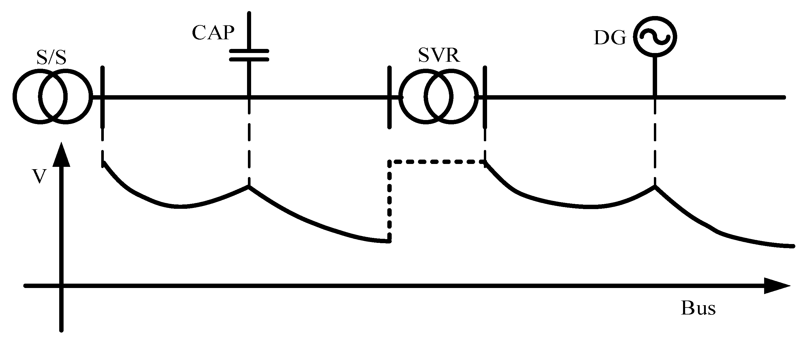
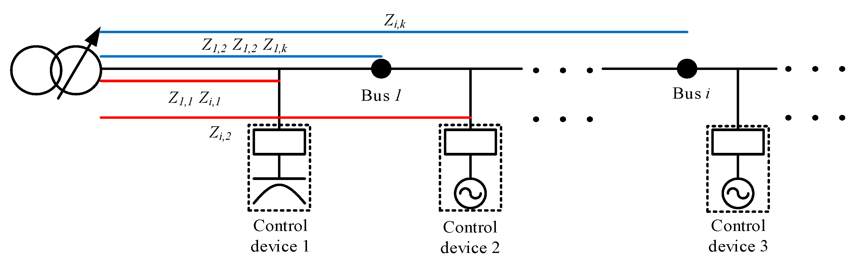
2. Voltage Equation Expressed as Simplified Linear Equation

The characteristics of the voltage control devices in the distribution system are derived as a simplified linear equation. The simplified linear equation is formulated as an optimization equation such as QP.

2.1. Simplified Linear Equation

The voltage of the distribution system is controlled by utilizing various voltage control devices. Figure 1 shows that the tap changing devices, such as OLTC and SVR, can control the entire voltage of a subarea, while the reactive power devices transform the voltage profile of the distribution systems. The capacitor bank and DG have a characteristic of increasing the voltage of the interconnected point in Figure 1. The SVR can increase the entire voltages of the downstream area as shown in Figure 1.
The voltage control devices are classified into three types, according to the voltage control characteristics. The voltage devices are divided into tap changing devices, i.e., OLTC and SVR, discrete reactive power devices, i.e., capacitors, and continuous reactive power devices, i.e., DGs. The tap changing devices can also be classified as discrete devices.
In voltage control, the voltage variation due to the voltage control devices can be considered separately. The estimated voltage can be derived from the measured voltage and the voltage variation of each control devices using the superposition principle. The estimated voltage can be expressed as the sum of the voltage variations of each control devices as shown in Equation (1).
V est = V mea + Δ V DG + Δ V Tap + Δ V CAP
where,
V est : estimated voltage,
V mea : measured voltage,
Δ V DG : voltage variation by DG,
Δ V Tap : voltage variation by tap changing device,
Δ V CAP : voltage variation by capacitor.
The voltage variation by output of DG is affected by the impedance of the distribution networks. The voltage variation at bus i by small active and reactive power of DG can be presented by Equation (2).
Δ V i , DG , j R i , j · Δ P DG , j + X i , j · Δ Q DG , j
where,
i : bus number,
j : DG number,
Δ V i , DG , j : voltage variation at bus i by the j -th DG,
R i . j : resistance at bus i by the j -th DG,
X i , j : reactance at bus i by the j -th DG,
Δ P DG , j : active power variation of the j -th DG,
Δ Q DG , j : reactive power variation of the j -th DG.
The section impedance is determined by the location of control devices and buses in Figure 2. For example, the voltage variation of bus i due to Control device 2 is determined by section impedance ( Z 1 , 2 ) between substation and Control device 2 as shown in Figure 1.
Generally, the DGs of a distribution system are operated as the maximum active power to maximize availability of DGs. Therefore, the voltages of buses are controlled by using reactive power of DGs without active power. The voltage variation due to small variation of reactive power of the j -th DG can be represented in Equation (3).
Δ V i , DG , j X i , j · Δ Q DG , j
The voltage variation by the reactive power of DGs on each bus can be expressed as the reactance for each reactive power of DG, as shown in Equation (4).
Δ V DG = X DG · [ Δ Q DG , 1 Δ Q DG , j Δ Q DG , m ] , X DG = [ X 1 , 1 X 1 , j X 1 , m X i , 1 X n , 1 X i , j X i , m X n , j X n , m ]
where,
m : total number of DGs,
Δ Q DG , j : reactive power variation of the j -th DG.
The voltage variation due to k -th tap changing device can be expressed by the voltage variation ( Δ V Tap , k ) and the load current variation ( Δ I Load , k ) caused by the changing tap, as shown in Equation (5).
Δ V i , Tap , k = Δ V Tap , k + Δ I Load , k · Z i , k
where,
k : tap changing device number,
Δ V i , Tap , k : voltage variation by taps of the k -th tap changing device,
Δ V Tap , k : voltage variation caused by tap changes,
Δ I Load , k : load current variation caused by tap changes,
Z i , k : impedance at bus i by the k -th tap changing device.
Since the voltage variation caused by tap change is small, the load current change is also small enough. Therefore, the voltage variation due to the k -th tap changing device can be represented in Equation (6).
Δ V i , Tap , k Δ V Tap , k
The tap changing devices can generally control the voltages of buses in the downstream section of the distribution system in Figure 3. However, the tap changing devices do not control the voltages of buses in the upstream section of the distribution system. Therefore, the control area factor ( α i , k ) of tap changing devices is applied, as shown in Equation (7).
Equation (7) shows the voltage variation by the tap changing devices. It can be expressed by the number of control taps of the tap changing device, the variation voltage per tap of the tap changing device, and the control area factor of the tap changing devices.
Δ V Tap = a Tap · [ V Tap , 1 · Δ T a p 1 V Tap , k · Δ T a p k V Tap , l · Δ T a p l ] ,   a Tap = [ α 1 , 1 α 1 , k α 1 , l α i , 1 α n , 1 α i , k α i , l α n , k α n , l ] α i , k = {   1 , b u s   i k   c o n t r o l   s e c t i o n     0 , b u s   i k   c o n t r o l   s e c t i o n
where,
l: total number of tap changing devices,
Δ Tap k : voltage variation per tap of the k -th tap changing device,
V Tap , k : the number of control taps of the k -th tap changing device,
α i , k : voltage factor at bus i of the k -th tap changing device.
Equation (8) shows that the voltage variation by the capacitor can be expressed as the number of control capacitor banks, the capacity per capacitor bank, and the reactance matrix of the distribution system.
Δ V CAP = X CAP · [ Q CAP , 1 · Δ n 1 Q CAP , p · Δ n p Q CAP , q · Δ n q ] ,   X CAP = [ X 1 , 1 X 1 , j X 1 , q X i , 1 X n , 1 X i , p X i , q X n , p X n , q ]
where,
p : capacitor bank number,
q : total number of capacitor bank,
Q CAP , p : capacity per capacitor bank of the p -th capacitor bank,
Δ n p : the number of control banks of the p -th capacitor bank.

2.2. Formulation of Objective Function for Optimization

For the voltage control operation of distribution systems, a basic method to maintain a nominal voltage is performed. This controls the voltages of the customer to be close to the nominal voltage without any voltage violation. Thus, in the case of voltage control for nominal voltage, the voltages of the distribution system can be stably operated.
In the case of voltage control to achieve the nominal voltage, the voltages of distribution systems are controlled to be close to the target voltage value, as shown in Equation (9).
m i n i = 1 N ( V i V target ) 2
where,
V target : target voltage.
Conservation voltage reduction (CVR) is a method of reducing the load energy consumed by controlling the voltages of buses in distribution systems [36]. The entire voltages of the distribution systems are controlled to be the closest to the minimum operating voltage within a range in which voltage violation does not occur. The voltage control for CVR can be performed using the proposed optimization technique. Since the entire voltage of a distribution system can be controlled close to the lowest voltage, the CVR effect can be maximized. In the case of the voltage control to achieve CVR, the references of the voltage control devices are obtained by solving the optimization equation, as shown in Equation (10).
m i n i = 1 N ( V i V m i n , limit ) 2
where,
V m i n , limit : minimum operating voltage limit.
There are four optimization constraints, which are as follows. The reactive power output range of DGs is shown in Equation (11).
Q DG , m i n , j Q DG , j 0 Δ Q DG , j Q DG , m a x , j Q DG , j 0
where,
Q DG , m i n , j : minimum limit of reactive power of the j -th DG,
Q DG , j 0 : initial reactive power output of the j -th DG,
Q DG , m a x , j : maximum limit of reactive power of the j -th DG.
The control range of the tap changing devices is shown in Equation (12).
Tap m i n , k Tap k 0 Δ Tap k Tap m a x , k Tap k 0
where,
Tap m i n , k : lowest tap position of the k -th tap changing device,
Tap k 0 : initial position of the k -th tap changing device,
Tap m a x , k : highest tap position of the k -th tap changing device.
The reactive power output range of capacitor banks is shown in Equation (13).
n CAP , p 0 Δ n CAP , p N CAP , p n CAP , p 0
where,
n CAP , p 0 : the number of initial inserted banks,
N CAP , p : maximum number of banks.
The voltage constraint due to the operating range of voltage control is expressed by Equation (14).
V m i n , limit V i V m a x , limit
where,
V m i n , limit : maximum operating voltage limit.

3. Quadratic Programming Formulation

In general, nonlinear programming (NLP) is used to derive the references for each device. As the objective function is expressed as a quadratic equation, it can be solved using QP. The standard form of QP can be expressed by Equation (15) [37,38]:
m i n 1 2 x T H x + f T x S . T { A · x b A e q · x = b e q l b x u b
The standard form of QP is generalized by applying control variables ( Δ ) as shown in Equation (16).
m i n 1 2 Δ T H Δ + f T Δ S . T { A · Δ b l b Δ u b
where
Δ : control variable.
In a given condition, the equality constraint does not exist, but an objective function and an inequality constraint are formulated.

3.1. Generalization of Objective Function

Using control variables, the generalization of the objective function can be expressed as shown in Equation (17)
x T H x + f T x = [ Δ Q DG , 1 Δ Q DG , m Δ T a p 1 Δ T a p l Δ n CAP , 1 Δ n CAP , q ] H [ Δ Q DG , 1 Δ Q DG , m Δ T a p 1 Δ T a p l Δ n CAP , 1 Δ n CAP , q ] + f T [ Δ Q DG , 1 Δ Q DG , m Δ T a p 1 Δ T a p l Δ n CAP , 1 Δ n CAP , q ]
The Hessian matrix H is composed as follows. It is obtained from the voltage factor of each device. Based on the device type, the Hessian matrix can be divided into three types, and it is determined by the product of the voltage factor of each control device. The Hessian matrix consists of 3 2 cases, as shown in Equation (18). The entire matrix has a size of ( m + l + q ) × ( m + l + q ) . The details of Equation (18) are explained in the Appendix A.
H = [ H 1 H 2 H 3 H 4 H 5 H 6 H 7 H 8 H 9 ]
Equation (19) is composed of the voltage factor of each control device, the measured voltage ( V mea , i ), and target voltage ( V target ). Equation (19) shows that the voltage factors that determine the objective function of voltage control are included.
f = [ i = 1 N { X i , 1 ( V mea , i V target ) } i = 1 N { X i , m ( V mea , i V target ) } i = 1 N { α i , 1 ( V mea , i V target ) } i = 1 N { α i , l ( V mea , i V target ) } i = 1 N { X i , 1 ( V mea , i V target ) } i = 1 N { X i , q ( V mea , i V target ) } ]

3.2. Generalization of Inequality Constraints

There are two inequality constraints. First, the voltage constraints of all buses in the distribution systems are generalized. The standard form of the first inequality constraint is presented as shown in Equation (26).
A x b
The generalization of the inequality constraints into the voltage control variables is expressed by the voltage variation equation to represent the control variation of each device, as shown in Equation (21).
A · [ Δ Q DG , 1 Δ Q DG , m Δ T a p 1 Δ T a p l Δ n CAP , 1 Δ n CAP , q ] [ V m a x , limit V mea , 1 V m a x , limit V mea , n V m i n , limit V mea , 1 V m i n , limit V mea , n ] A = [ X 1 , 1 X 1 , m X n , 1 X n , m α 1 , 1 α 1 , l α n , 1 α N , l X 1 , 1 X 1 , q X n , 1 X n , q X 1 , 1 X 1 , m X n , 1 X n , m α 1 , 1 α 1 , l α n , 1 α N , l X 1 , 1 X 1 , q X n , 1 X n , q ]
The second inequality constraint is the control range of voltage control devices. Equation (22) shows the standard form of inequality constraint.
l b x u b
The inequality constraint is generalized by using control variables in Equation (23).
[ Q DG , m i n , 1 Q DG , 1 0 Q DG , m i n , m Q DG , m 0 Tap m i n , 1 Tap 1 0 Tap m i n , l Tap l 0 n CAP , 1 0 n CAP , q 0 ] [ Δ Q DG , 1 Δ Q DG , m Δ Tap 1 Δ Tap l Δ n CAP , 1 Δ n CAP , q ] [ Q DG , m a x , 1 Q DG , 1 0 Q DG , m a x , m Q DG , m 0 Tap m a x , 1 Tap 1 0 Tap m a x , l Tap l 0 N CAP , 1 n CAP , 1 0 N CAP , q n CAP , q 0 ]

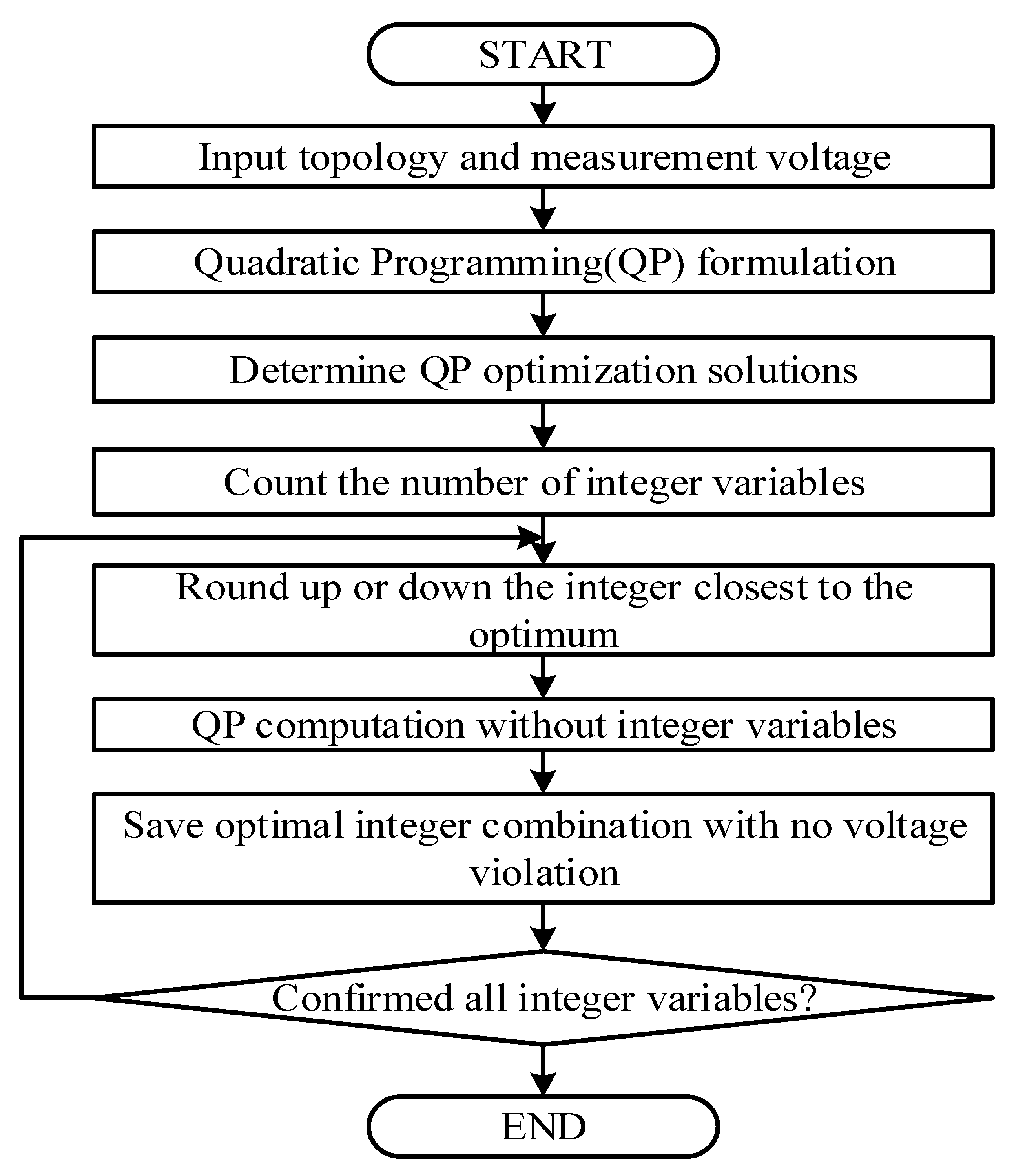
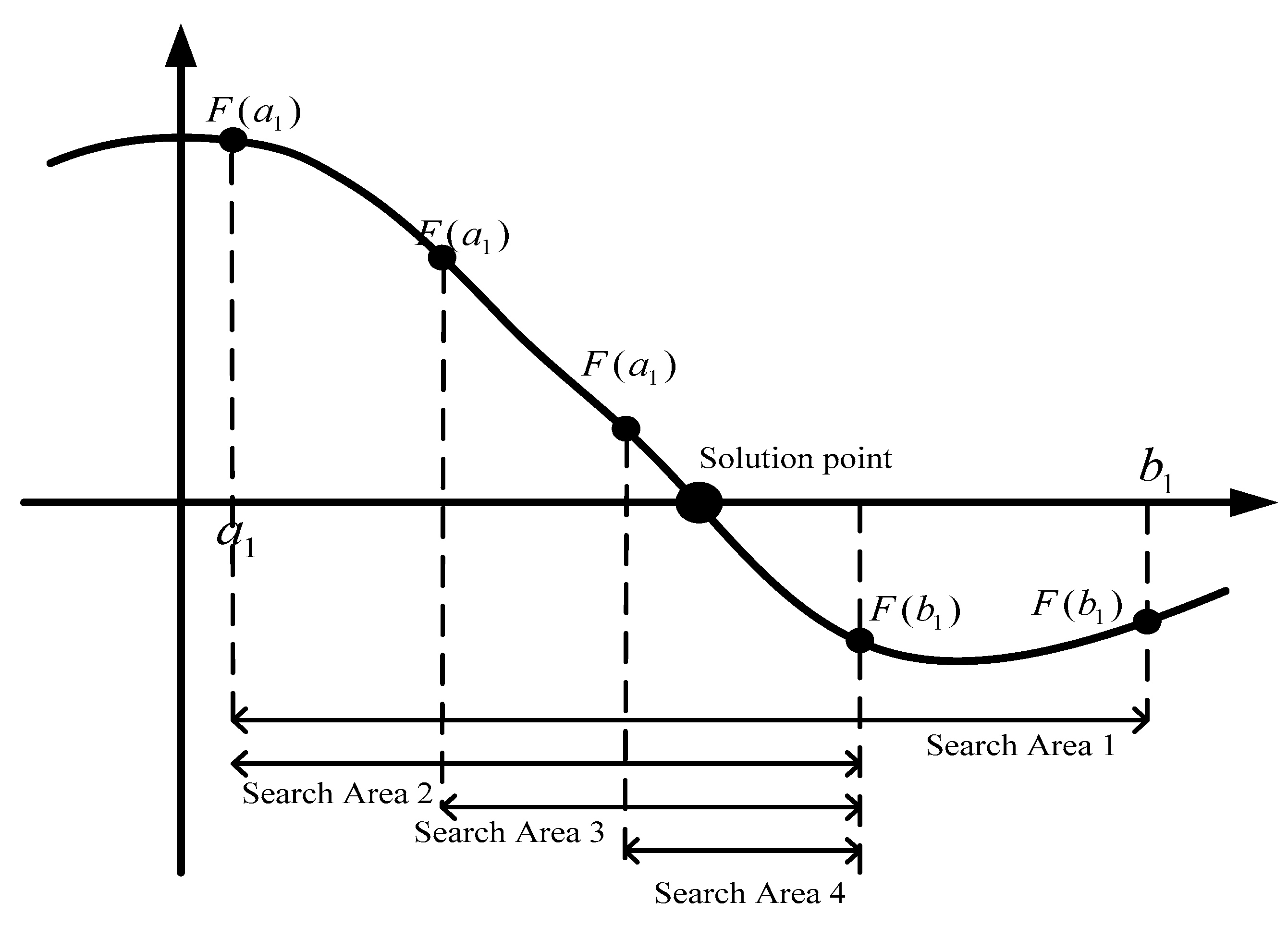
3.3. Approximation Method of MIQP
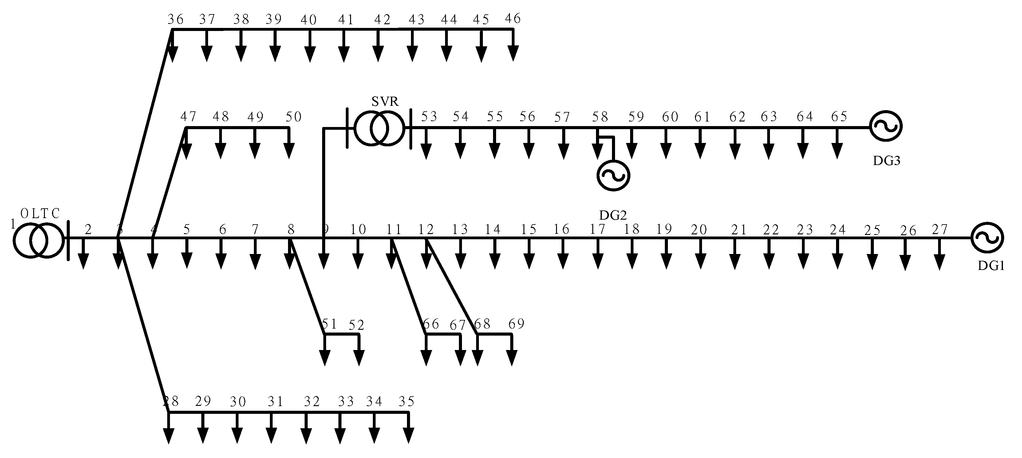
The MIQP solution can be obtained by following the process as shown in Figure 4. Figure 4 shows the flowchart of MIQP implementation. A general QP is used to obtain the continuous solution for all control variables. In order to derive the solution, the integer variables are rounded up or down using the approximation method. The integer solutions obtained from the approximation method are fixed, and QP is performed again for the variables excluding the integer variables. The solution when the objective function index value is the smallest is found for all possible integer variables.
To determine whether the proposed method is accurate, a simple method was chosen to derive the optimal solution. Therefore, among all the global search methods, the bisection method was used. In this method, an algorithm repeatedly bisects the interval contains a solution, and then selects the subinterval containing the solution. As this method sets the intervals on the premise that a solution exists, it is the most suitable when the equation is simple, and finding the solution. The solution interval is derived using the bisection method as shown in Figure 5. The intervals are sequentially narrowed, thereby going towards the optimal solution [39]. This method is simple, but, in comparison with the other methods, it has slow computation.

4. Case Studies

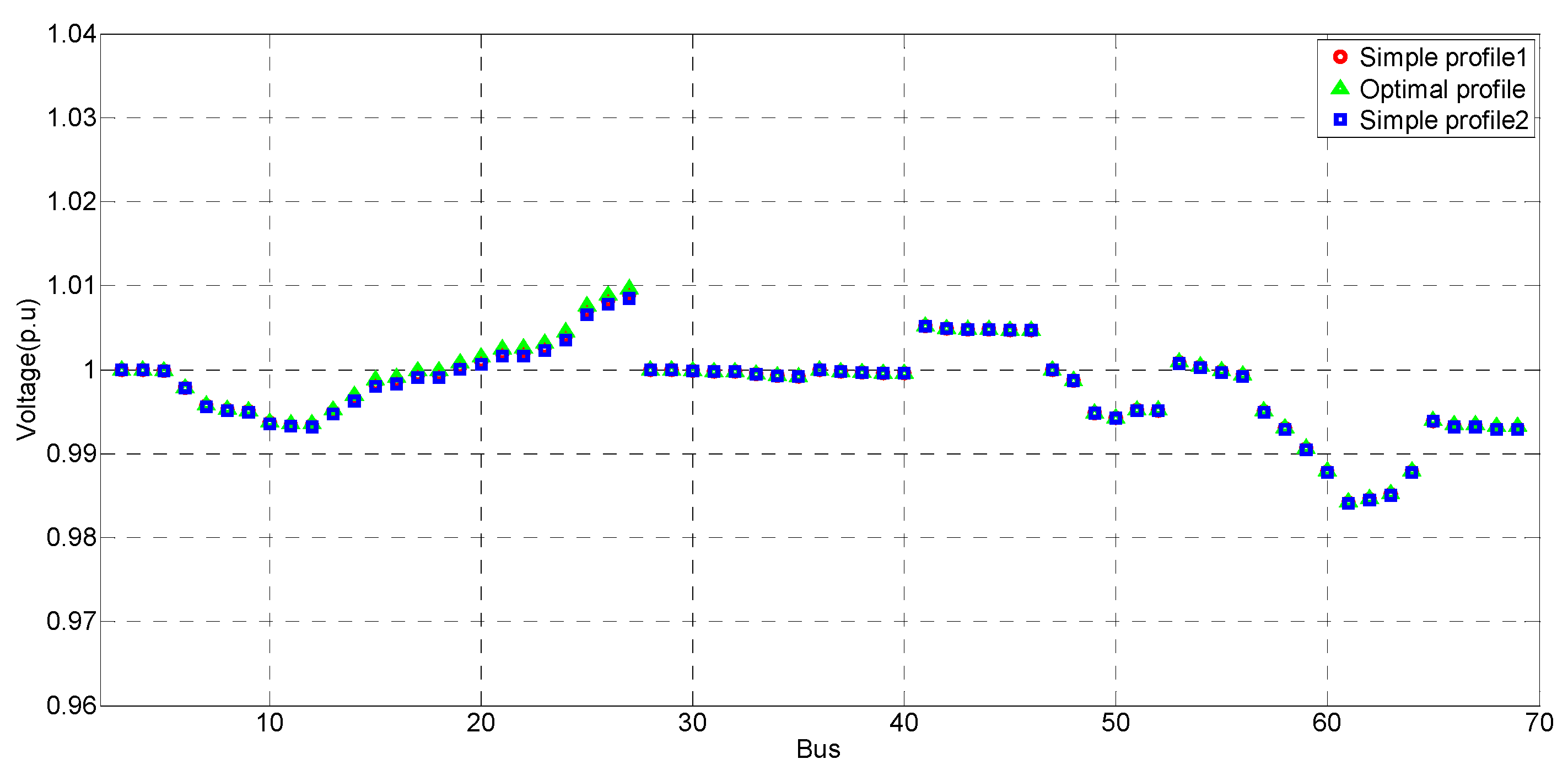
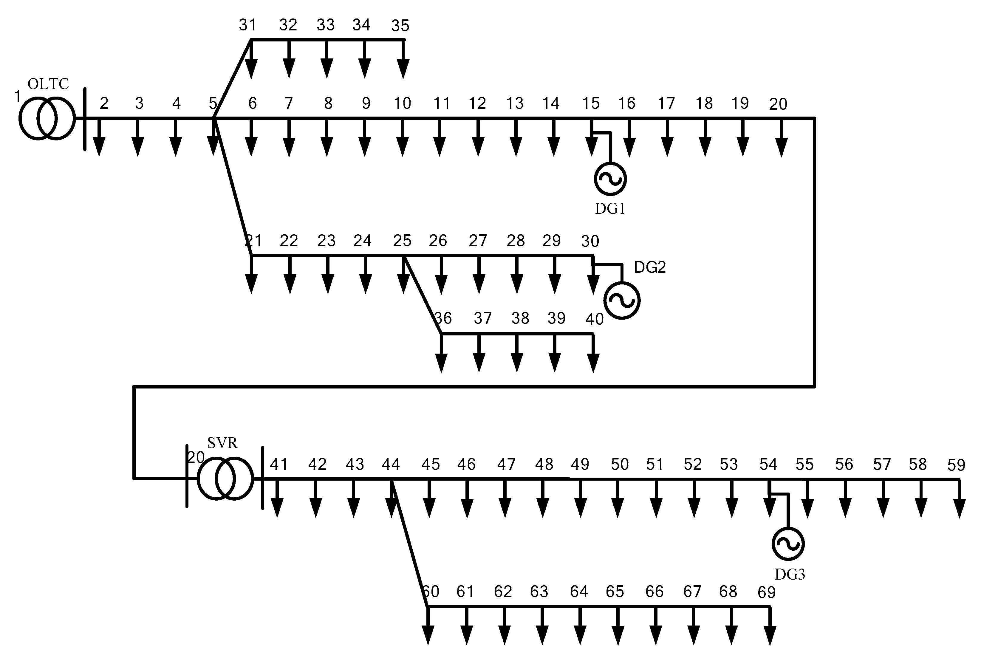
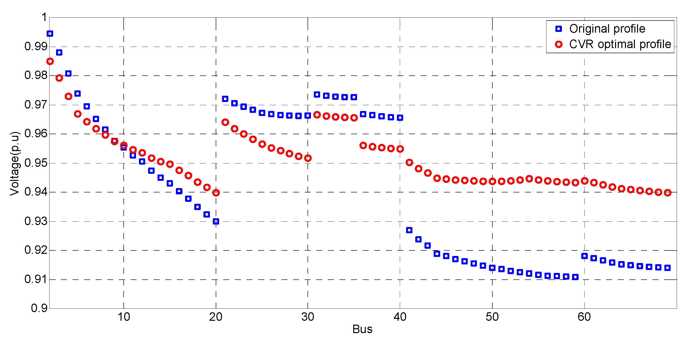
4.1. Simulation of Case Study 1

The simulation was conducted using the distribution networks, as shown in Figure 6. Table 1 details the system configuration.
A final solution can include error, as the reference is derived using a simplified linear equation. To compare the result of the error, simulation was performed using different initial conditions.

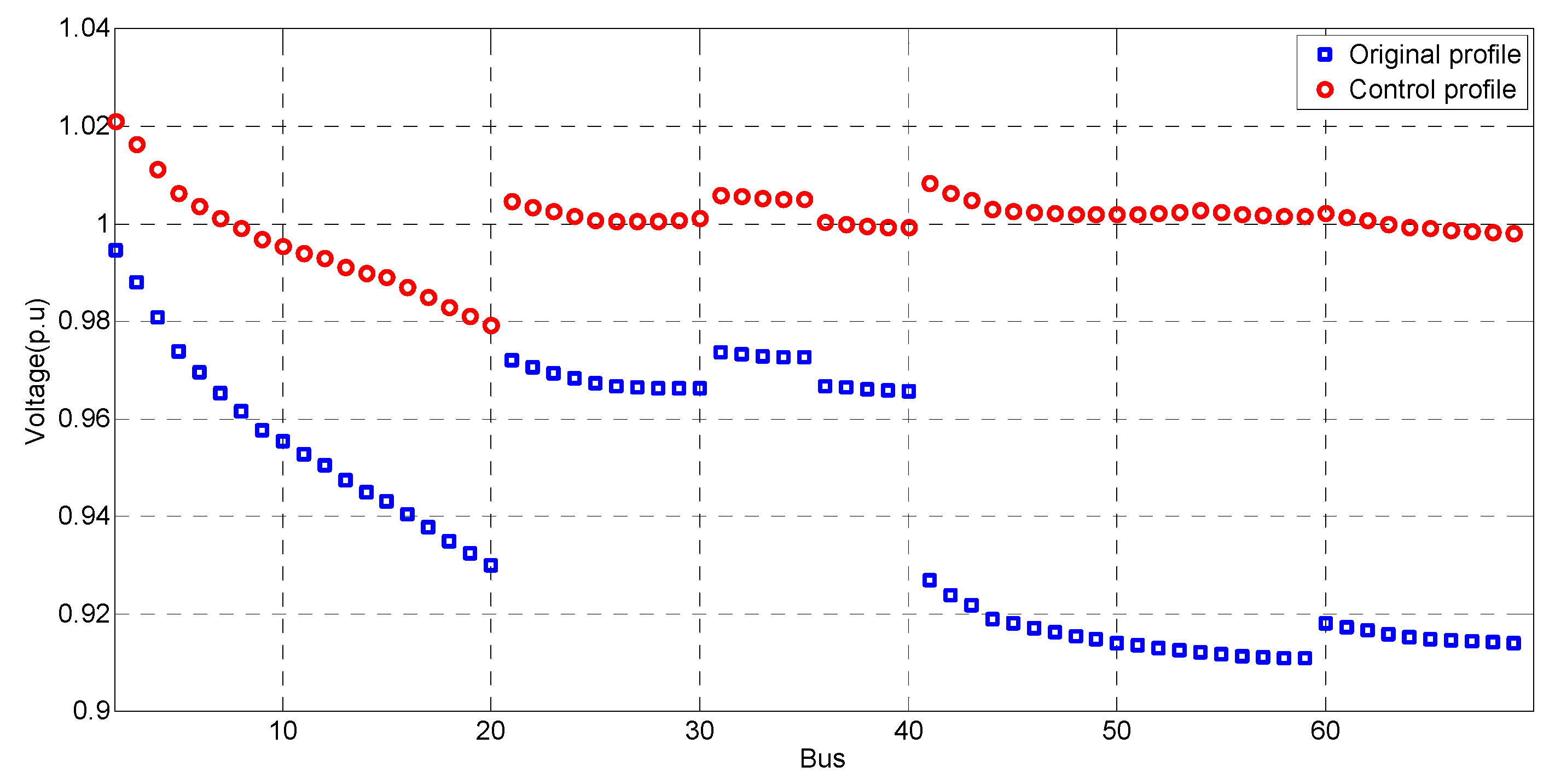
4.1.1. Voltage Control for CVR

Initially, continuous control references were obtained without limitation of integer variables. QP was used to find the continuous control references. Table 2 presents the continuous control references obtained through QP.
The references of tap changing devices are not integer variables. To express the objective function index (performance index) as a small value, we multiplied it by 10 4 : ( V i V m i n , limit ) 2 × 10 4 = 199.9426 . Figure 7 shows the voltage profile before (original profile) and after (CVR optimal profile) control.
The continuous control references obtained above were converted into discrete variables (integer variable) to obtain the final reference. Table 3 presents the final control references, while Figure 8 shows the final voltage profile.
If the control variation range is large, the difference between the results of the simplified linear equation and the power flow calculation can increase. Therefore, the control variation range was reduced to derive the appropriate result. To reduce the control variation range, this paper assumed that the output of the reactive power device was 0.5 MVAR. The results were obtained by reflecting the initial output, as presented in Table 4.
The results from each initial condition case were compared with the global optimum based on the power flow calculation. While the interval of the solution is reducing, the solution is derived through a global search using the bisection method [39]. Table 5 presents the results of the global optimum, while Figure 9 shows the voltage profile in distribution network of case study 1. ‘Simple profile1’ and ‘Simple profile2’ indicate the results derived from the initial conditions 1 and 2, respectively. ‘Optimal profile’ was obtained through the bisection method. In initial condition 2, the variation of the reactive power is smaller than that of initial condition 1, because initial reactive power of DGs is given. Figure 9 shows that result of less control change of the DG is closer to the global optimum.
Table 6 compares the results of the global optimum and initial condition.

4.1.2. Voltage Control for Nominal Voltage

In the same simulation system, the continuous reference was obtained through QP optimization to control voltage for nominal voltage. Table 7 details the continuous optimum results, while Figure 10 shows the voltage profile for the control results.
The continuous control reference was changed into a discrete variable to obtain the final reference. Table 8 presents the control results, while Figure 11 shows the initial voltage profile and the final voltage profile by the control references.
Table 9 presents the control results when the initial output of the DGs is assumed to be 0.5 MVAR.
Table 10 lists the results obtained through the global optimum, while Figure 12 compares the voltage control results for each initial output condition in the distribution network of case study 1.
Table 11 shows that the narrower the control variation is, the closer it is to the global optimum.

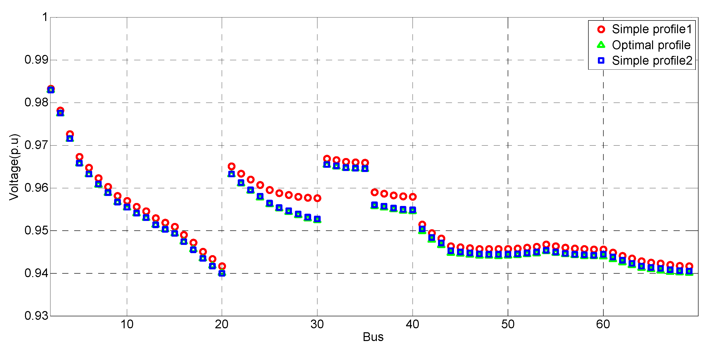
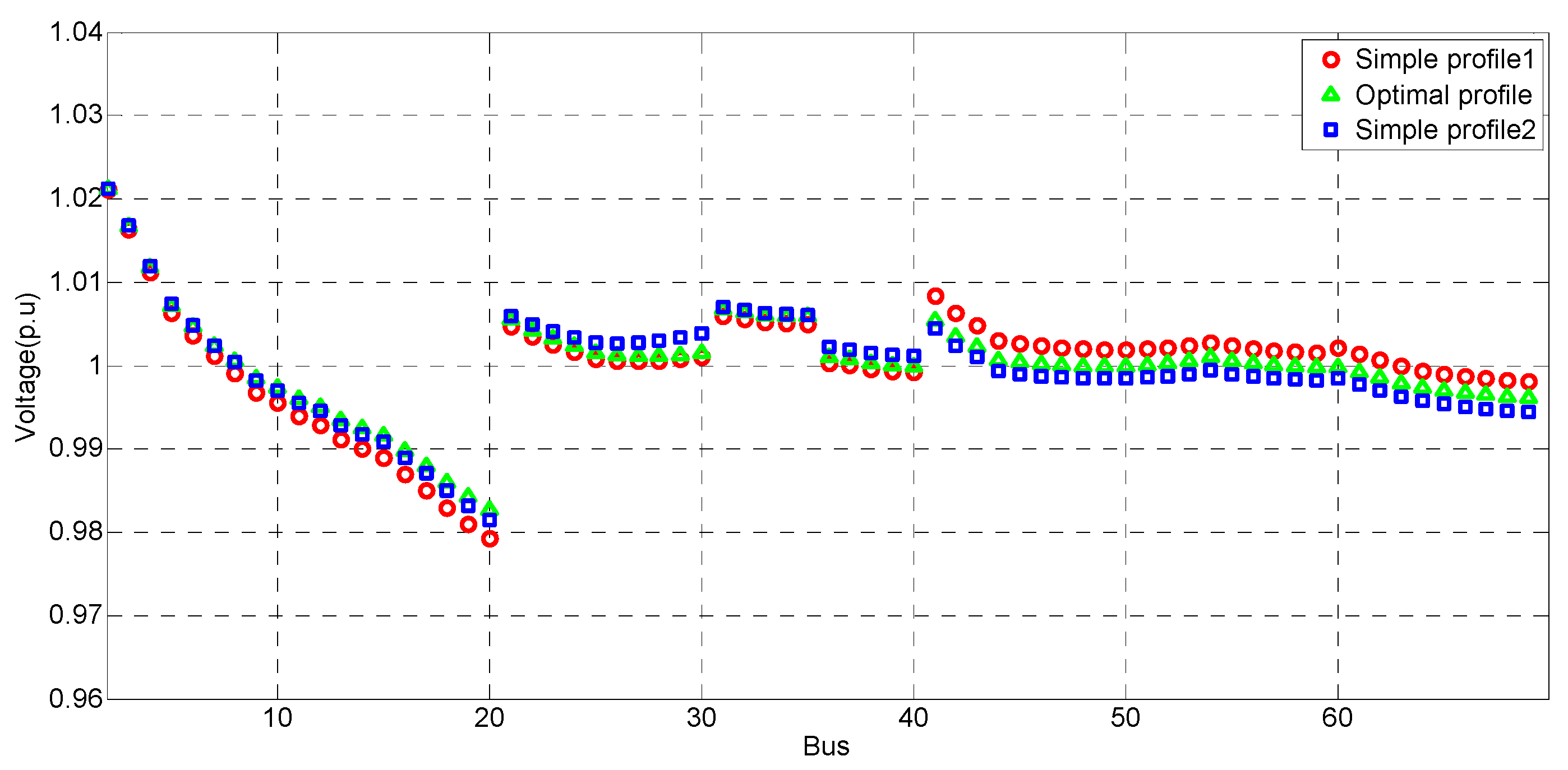
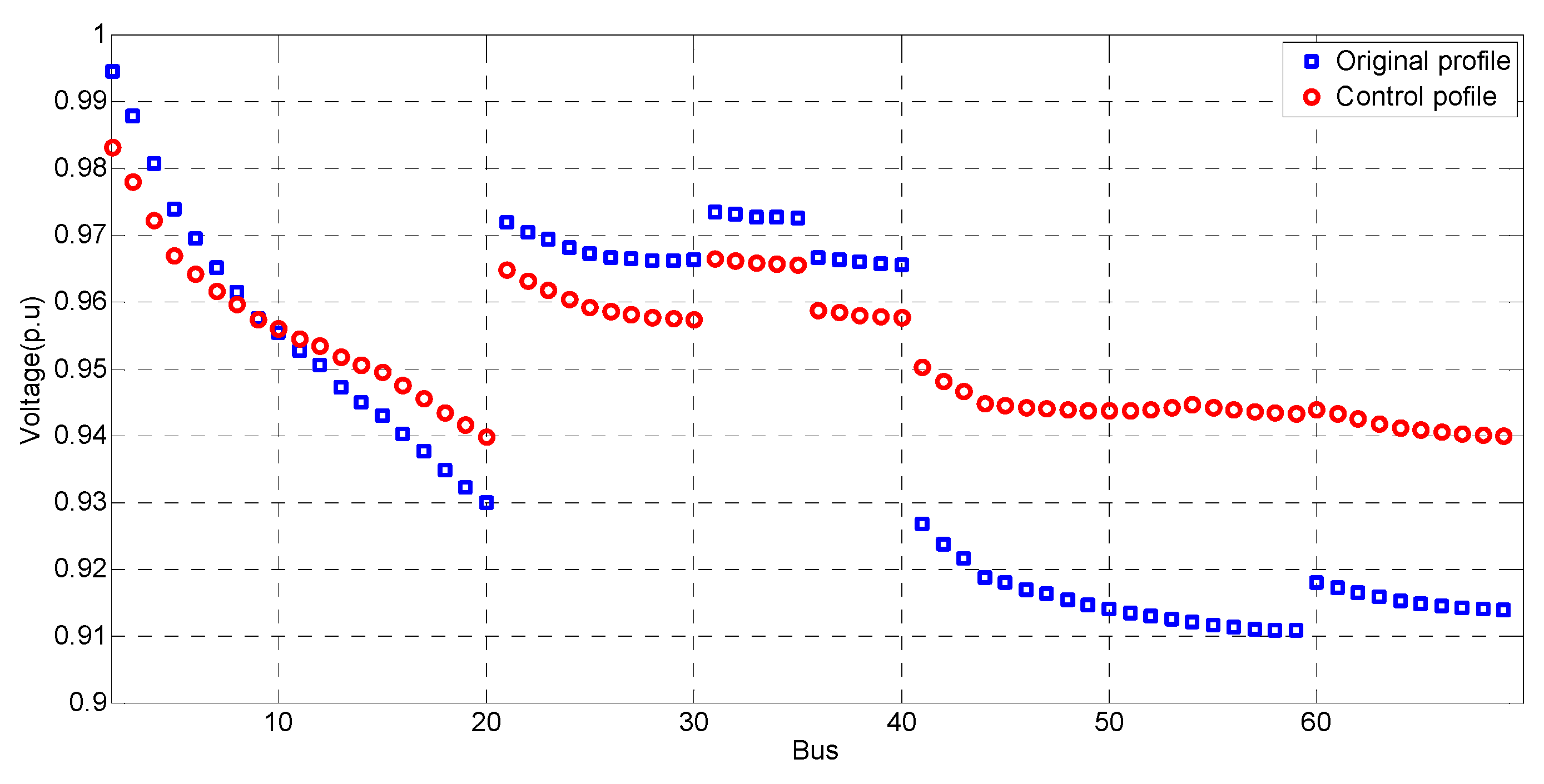
4.2. Simulation of Case Study 2

The case study was simulated using the modified IEEE 69-bus radial distribution system, as shown in Figure 13 [40]. DG and SVR were added to the lateral branch with the largest voltage drop in the system network. Table 12 shows the system configuration.

4.2.1. Voltage Control for CVR

Figure 14 and Table 13 show the voltage control results for the CVR in the distribution network of case study 2. Figure 14 compares the results of the global optimum and initial condition. It is confirmed that the result of initial condition 2 is closer to the optimal result.

4.2.2. Voltage Control for Nominal Voltage

Figure 15 and Table 14 show the voltage control results for the nominal voltage in the distribution network of case study 2. In the voltage control for the nominal voltage, the result of initial condition 2 is also closer to the optimal result.

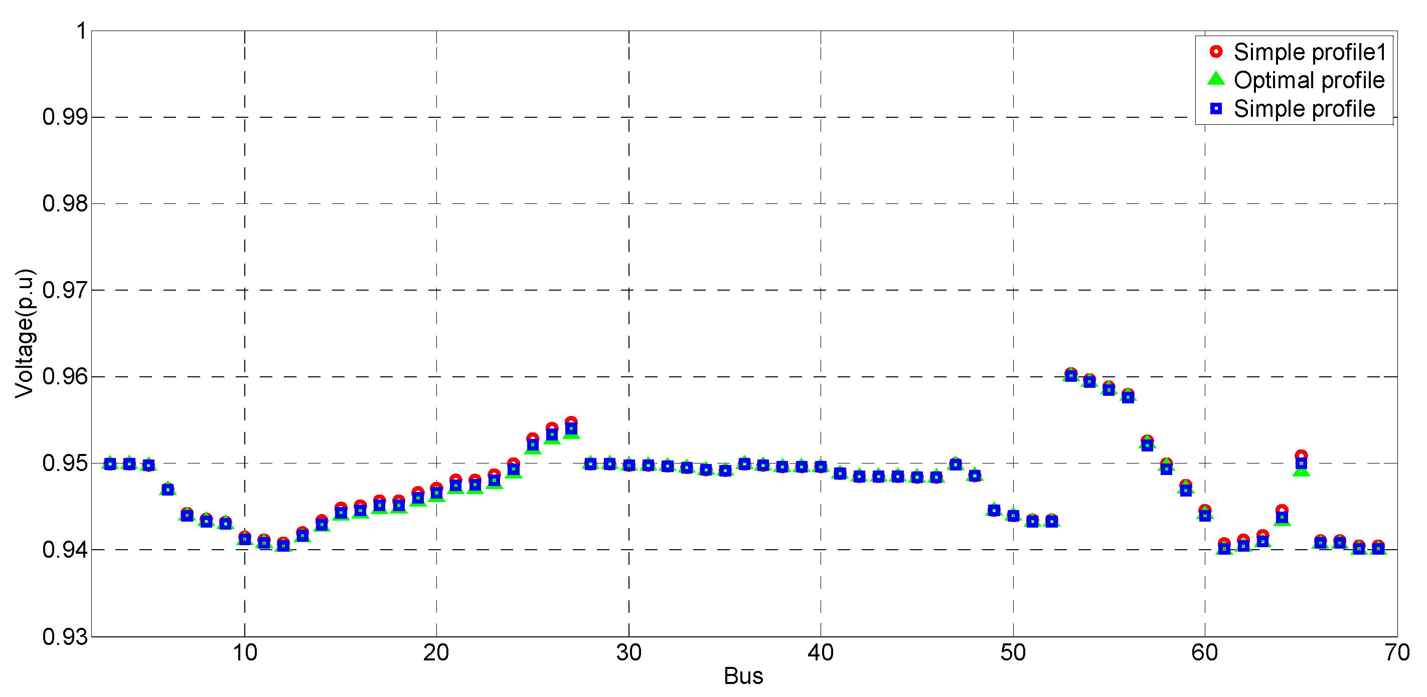
4.3. Simulation Analysis

The proposed method was used to derive the control reference using the objective function derived from a simplified linear equation. As such, the control result differs from the global optimum. However, as the case study demonstrates, the narrower control variation has the smaller error due to the simplified linear equation. If the control variation becomes large, more error in the control occurs. In real-time voltage control, as control is performed repeatedly in a relatively short cycle, the state change of the system according to the control cycle is inevitably small. If the state change of the system is small, then the variation due to control is also small. Therefore, the error due to the simplified calculation can be ignored. Accordingly, the proposed method is considered to not only reduce the computation burden in actual operation but also enable the derivation of the optimal control reference.
The proposed voltage control optimization technique using measured data can be applied to a practical system. However, the measured data includes measurement errors. Therefore, to apply the proposed voltage control optimization to the practical system, measurement errors must be taken into account. Since the proposed voltage control technique proposes a real-time control method, it is considered that measurement errors in the practical system are negligible because the state change is small during the control cycle.

5. Conclusions

Owing to the increase in the use renewable energy, the voltage control of distribution systems is undergoing numerous changes. In particular, if DG is actively utilized for voltage control in distribution systems, the voltage control method is also changed accordingly. Various techniques have been applied, including modifications to the existing LDC method or new techniques. The optimization method is also one of the methods applied to voltage control. Accordingly, this paper proposed a real-time voltage and reactive power control method using nonlinear optimization. The proposed method determines the control reference that produces an optimal voltage profile. Rather than using complex power flow calculations, the characteristics of the voltage control devices in the distribution systems were expressed as a simplified linear equation for fast computation. After being expressed as simplified linear equations, voltage control characteristics were formulated through QP optimization. The inequality constraints were generalized using the voltage operating range of the distribution system and the output range of each device. The optimal references were derived using the approximation method. The proposed method results were compared with the optimal results of a global search method. The simulation demonstrates that under the given conditions, the derived results were almost identical to the optimal solution.

Author Contributions

S.-I.G. prepared the manuscript and implemented the theory and simulations. J.-H.C. supervised the study and discussed the results. S.-Y.Y. and S.-J.A. analyzed the simulation results and commented on the manuscript. All authors have read and agreed to the published version of the manuscript.

Funding

This research was supported by Korea Electric Power Corporation (Grant number: R18XA04). This research was supported by the Korean Institute of Energy Technology Evaluation and Planning (KETEP) and the Ministry of Trade, Industry and Energy (MOTIE) of Republic of Korea (No. 2019381010001B).

Conflicts of Interest

The authors declare no conflict of interest.

Appendix A

H 1 is determined by the reactance of the distribution systems, and the matrix size m × m is the square of the number of DGs.
H 1 = [ i = 1 N X i , 1 2 i = 1 N ( X i , m X i , 1 ) i = 1 N ( X i , 1 X i , m ) i = 1 N ( X i , m 2 ) ]
H 2 is determined by the voltage factor of tap changing devices and DGs, and the matrix size l × m is the product of the number of DGs and the number of tap changing devices.
H 2 = [ i = 1 N ( α i , 1 X i , 1 ) i = 1 N ( α i , l X i , 1 ) i = 1 N ( α i , 1 X i , m ) i = 1 N ( a i , l X i , m ) ]
H 3 is determined by the reactance of the distribution systems, and the matrix size q × m is the product of the number of capacitors and the number of DGs.
H 3 = [ i = 1 N ( X i , 1 X i , 1 ) i = 1 N ( X i , q X i , 1 ) i = 1 N ( X i , 1 X i , m ) i = 1 N ( X i , q X i , m ) ]
H 4 is determined by the voltage factor of DGs and tap changing devices, and the matrix size m × l is the product of the number of DGs and the number of tap changing devices.
H 4 = [ i = 1 N ( X i , 1 α i , 1 ) i = 1 N ( X i , m α i , 1 ) i = 1 N ( X i , 1 α i , l ) i = 1 N ( X i , m α i , l ) ]
H 5 is determined by the control area factors of the tap changing devices, and the matrix size l × l is the square of the number of tap changing devices.
H 5 = [ i = 1 N ( α i , 1 2 ) i = 1 N ( α i , l α i , 1 ) i = 1 N ( α i , 1 α i , l ) i = 1 N ( α i , l 2 ) ]
H 6 is determined by the voltage factor of capacitors and tap changing devices, and the matrix size q × l is the product of the number of capacitors and the number of tap changing devices.
H 6 = [ i = 1 N ( X i , 1 α i , 1 ) i = 1 N ( X i , q α i , 1 ) i = 1 N ( X i , 1 α i , l ) i = 1 N ( X i , q α i , l ) ]
H 7 is determined by the voltage reactance of the distribution systems, and the matrix size m × q is the product of the number of DGs and the number of capacitors.
H 7 = [ i = 1 N ( X i , 1 X i , 1 ) i = 1 N ( X i , m X i , 1 ) i = 1 N ( X i , 1 X i , q ) i = 1 N ( X i , m X i , q ) ]
H 8 is determined by the voltage factor of the tap changing devices and capacitors, and the matrix size l × q is the product of the number of capacitors and tap controllers.
H 8 = [ i = 1 N ( α i , 1 X i , 1 ) i = 1 N ( α i , l X i , 1 ) i = 1 N ( α i , 1 X i , q ) i = 1 N ( a i , l X i , q ) ]
H 9 is determined by the reactance of the distribution systems, and the matrix size q × q is the square of the number of capacitors.
H 9 = [ i = 1 N X i , 1 2 i = 1 N ( X i , q X i , 1 ) i = 1 N ( X i , 1 X i , q ) i = 1 N ( X i , q 2 ) ]

References

  1. Nam-Koong, W.; Jang, M.J.; Lee, S.W.; Seo, D.W. A study on the operation of distribution system for increasing grid-connected distributed generation. J. Korean Inst. Illum. Electr. Install. Eng. 2014, 28, 83–88. [Google Scholar]
  2. Moon, W.S.; Cho, S.M.; Shin, H.S.; Lee, H.T.; Han, W.K.; Choo, D.W.; Kim, J.C. The study on permissible capacity of distributed generation considering voltage variation and load capacity at the LV distribution power system. KIEE Int. Trans. Power Eng. P 2010, 59, 100–105. [Google Scholar]
  3. Liu, X.; Aichhorn, A.; Liu, L.; Li, H. Coordinated control of distributed energy storage system with tap changer transformers for voltage rise mitigation under high photovoltaic penetration. IEEE Trans. Smart Grid 2012, 3, 897–906. [Google Scholar] [CrossRef]
  4. Comfort, R.; Mansoor, A.; Sundaram, A. Power quality impact of distributed generation: Effect on steady state voltage regulation. In Proceedings of the PQA 2001 North. America Conference, Pittsburgh, PA, USA, 12–14 June 2001. [Google Scholar]
  5. Li, Y.W.; Kao, C.N. An accurate power control strategy for power-electronics-interfaced distributed generation units operating in a low-voltage multibus microgrid. IEEE Trans. Power Electr. 2009, 24, 2977–2988. [Google Scholar]
  6. Turitsyn, K.; Šulc, P.; Backhaus, S.; Chertkov, M. Local control of reactive power by distributed photovoltaic generators. In Proceedings of the 2010 First IEEE International Conference on Smart Grid Communications (SmartGridComm), Gaithersbury, MD, USA, 4–6 October 2010; IEEE: Piscataway, NL, USA, 2010. [Google Scholar]
  7. Elnashar, M.; Kazerani, M.; El Shatshat, R.; Salama, M.A. Comparative evaluation of reactive power compensation methods for a stand-alone wind energy conversion system. In Proceedings of the 2008. IEEE Power Electronics Specialists Conference PESC, Rhodes, Greece, 15–19 June 2008; IEEE: Piscataway, NL, USA, 2008. [Google Scholar]
  8. Thomson, M. Automatic voltage control relays and embedded generation. Power Eng. J. 2000, 14, 71–76. [Google Scholar] [CrossRef]
  9. Hiscock, J.; Hiscock, N.; Kennedy, A. Advanced voltage control for networks with distributed generation. In Proceedings of the19th International Conference on Electricity Distribution, Vienna, Austria, 21–24 May 2007. [Google Scholar]
  10. Viawan, F.A.; Sannino, A.; Daalder, J. Voltage control with on-load tap changers in medium voltage feeders in presence of distributed generation. Electr. Power Syst. Res. 2007, 77, 1314–1322. [Google Scholar] [CrossRef]
  11. Choi, J.H.; Kim, J.C. Advanced voltage regulation method of power distribution systems interconnected with dispersed storage and generation systems. IEEE Trans. Power Deliv. 2001, 16, 329–334. [Google Scholar] [CrossRef]
  12. Azzouz, M.A.; Farag, H.E.; El-Saadany, E.F. Fuzzy-based control of on-load tap changers under high penetration of distributed generators. In Proceedings of the 2013 3rd International Conference on Electric Power and Energy Conversion Systems (EPECS), Istanbul, Turkey, 2–4 October 2013; IEEE: Piscataway, NL, USA, 2013. [Google Scholar]
  13. Elkhatib, M.E.; Shatshat, R.E.; Salama, M.M.A. Decentralized reactive power control for advanced distribution automation systems. IEEE Trans. Smart Grid 2012, 3, 1482–1490. [Google Scholar] [CrossRef]
  14. Calderaro, V.; Conio, G.; Galdi, V.; Massa, G.; Piccolo, A. Optimal decentralized voltage control for distribution systems with inverter-based distributed generators. IEEE Trans. Power Syst. 2014, 29, 230–241. [Google Scholar] [CrossRef]
  15. Tsuji, T.; Hashiguchi, T.; Goda, T.; Horiuchi, K.; Kojima, Y. Autonomous decentralized voltage profile control using multi-agent technology considering time-delay. In Proceedings of the 2009 Transmission &Distribution Conference &Exposition: Asia and Pacific, Seoul, Korea, 20 June 2009; IEEE: Piscataway, NL, USA, 2009. [Google Scholar]
  16. Robbins, B.A.; Hadjicostis, C.N.; Domínguez-García, A.D. A two-stage distributed architecture for voltage control in power distribution systems. IEEE Trans. Power Syst. 2013, 28, 1470–1482. [Google Scholar] [CrossRef]
  17. Carvalho, P.M.S.; Correia, P.F.; Ferreira, L.A.F.M. Distributed reactive power generation control for voltage rise mitigation in distribution networks. IEEE Trans. Power Syst. 2008, 23, 766–772. [Google Scholar] [CrossRef]
  18. Zoka, Y.; Yorino, N.; Watanabe, M.; Kurushima, T. An optimal decentralized control for voltage control devices by means of a multi-agent system. In Proceedings of the 2014 Power Systems Computation Conference (PSCC 2014), Wroclaw, Poland, 18–22 August 2014; IEEE: Piscataway, NL, USA, 2014. [Google Scholar]
  19. Hatta, H.; Kobayashi, H. A study of centralized voltage control method for distribution system with distributed generation. In Proceedings of the 19th International Conference on Electricity Distribution (CIRED), Vienna, Austria, 21–24 May 2007. [Google Scholar]
  20. Thornley, V. Field experience with active network management of distribution networks with distributed generation. In Proceedings of the 19th International Conference on Electricity Distribution, Vienna, Austria, 21–24 May 2007. [Google Scholar]
  21. Thornley, V.; Hill, J.; Lang, P.; Reid, D. Active network management of voltage leading to increased generation and improved network utilisation. In Proceedings of the CIRED Seminar 2008, Frankfurt, Germany, 23–24 June 2008. [Google Scholar]
  22. Caldon, R.; Spelta, S.; Prandoni, V.; Turri, R. Co-ordinated voltage regulation in distribution networks with embedded generation. In Proceedings of the 18th International Conference on Electricity Distribution, Turin, Italy, 6–9 June 2005. [Google Scholar]
  23. Hird, C.M.; Leite, H.; Jenkins, N.; Li, H. Network voltage controller for distributed generation. IEE Proc.-Gener. Transm. Distrib. 2004, 151, 150–156. [Google Scholar] [CrossRef]
  24. Santoso, S.; Saraf, N.; Venayagamoorthy, G.K. Intelligent techniques for planning distributed generation systems. In Proceedings of the 2007 IEEE Power Engineering Society General Meeting, Tampa, FL, USA, 24–28 June 2007; IEEE: Piscataway, NL, USA, 2007. [Google Scholar]
  25. Sugimoto, J.; Yokoyama, R.; Fukuyama, Y.; Silva, V.V.R.; Sasaki, H. Coordinated allocation and control of voltage regulators based on reactive tabu search. In Proceedings of the 2005 IEEE Russia Power Tech, PowerTech, St. Peteersburg, Russia, 27–30 June 2005; IEEE: Piscataway, NL, USA, 2005. [Google Scholar]
  26. Hu, Z.; Wang, X.; Chen, H.; Taylor, G. Volt/VAr control in distribution systems using a time-interval based approach. IEE Proc.-Gener. Transm. Distrib. 2003, 150, 548–554. [Google Scholar] [CrossRef]
  27. Shalwala, R.A.; Bleijs, J.A.M. Voltage control scheme using Fuzzy Logic for residential area networks with PV generators in Saudi Arabia. In Proceedings of the 2010 Joint International Conference on Power Electronics, Drives and Energy Systems (PEDES) &2010 Power India, New Delhi, India, 20–23 December 2010; IEEE: Piscataway, NL, USA, 2010. [Google Scholar]
  28. Liang, R.H.; Liu, X.Z. Neuro-fuzzy based coordination control in a distribution system with dispersed generation system. In Proceedings of the 2007 International Conference on Intelligent Systems Applications to Power Systems, ISAP, Koahsiung, Taiwan, 5–8 November 2007; IEEE: Piscataway, NL, USA, 2007. [Google Scholar]
  29. Kim, G.W.; Lee, K.W. Coordination control of ULTC transformer and STATCOM based on an artificial neural network. IEEE Trans. Power Syst. 2005, 20, 580–586. [Google Scholar] [CrossRef]
  30. Ausavanop, O.; Chaitusaney, S. Coordination of dispatchable distributed generation and voltage control devices for improving voltage profile by Tabu Search. In Proceedings of the 2011 8th International Conference on Electrical Engineering/Electronics, Computer, Telecommunications and Information Technology (ECTI-CON), Khon Kaen, Thailand, 17–19 May 2011; IEEE: Piscataway, NL, USA, 2011. [Google Scholar]
  31. Rahideh, A.; Gitizadeh, M.; Rahideh, A. Fuzzy logic in real time voltage/reactive power control in FARS regional electric network. Electr. Power Syst. Res. 2006, 76, 996–1002. [Google Scholar] [CrossRef]
  32. Spatti, D.H.; Usida, W.F.; Da Silva, I.N. Real-time voltage regulation in power distribution system using fuzzy control. IEEE Trans. Power Deliv. 2010, 25, 1112–1123. [Google Scholar] [CrossRef]
  33. Cao, J.; Zhang, W.; Xiao, Z.; Hua, H. Reactive power optimization for transient voltage stability in energy internet via deep reinforcement learning approach. Energies 2019, 12, 1556. [Google Scholar] [CrossRef] [Green Version]
  34. Wu, J.; Shi, C.; Shao, M.; An, R.; Zhu, X.; Huang, X.; Cai, R. Reactive power optimization of a distribution system based on scene matching and deep belief network. Energies 2019, 12, 3246. [Google Scholar] [CrossRef] [Green Version]
  35. Jiang, F.; Zhang, Y.; Zhang, Y.; Liu, X.; Chen, C. An adaptive particle swarm optimization algorithm based on guiding strategy and its application in reactive power optimization. Energies 2019, 12, 1690. [Google Scholar] [CrossRef] [Green Version]
  36. Wang, Z.; Wang, J. Review on implementation and assessment of conservation voltage reduction. IEEE Trans. Power Syst. 2014, 29, 1306–1315. [Google Scholar] [CrossRef]
  37. Jensen, P.A.; Bard, J.F. Operations Research Models and Methods; John Wiley & Sons Incorporated: Hoboken, NJ, USA, 2003; Volume 1. [Google Scholar]
  38. Wright, S.; Nocedal, J. Numerical Optimization; Springer: New York, NY, USA, 1999; Volume 35, p. 7. [Google Scholar]
  39. Burden, R.L.; Faires, J.D. Numerical Analysis; Brooks/Cole: Boston, MA, USA, 2001. [Google Scholar]
  40. Baran, M.E.; Wu, F.F. Optimal capacitor placement on radial distribution systems. IEEE Trans. Power Deliv. 1989, 4, 725–734. [Google Scholar] [CrossRef]
Figure 1. Voltage profile caused by voltage devices.
Energies 13 03334 g001
Figure 2. The section impedance by location of distributed generations (DGs) and nodes.
Energies 13 03334 g002
Figure 3. Control area of tap changing devices.
Energies 13 03334 g003
Figure 4. Flowchart of process of the MIQP approximation method.
Energies 13 03334 g004
Figure 5. Illustration of bisection method [39].
Energies 13 03334 g005
Figure 6. Distribution networks for case study 1.
Energies 13 03334 g006
Figure 7. Voltage profile by continuous control reference for CVR.
Energies 13 03334 g007
Figure 8. Voltage profile by final reference for CVR.
Energies 13 03334 g008
Figure 9. Comparison of the results of global optimum and initial condition.
Energies 13 03334 g009
Figure 10. Voltage profile by continuous control reference for nominal voltage.
Energies 13 03334 g010
Figure 11. Voltage profile by final reference for nominal voltage.
Energies 13 03334 g011
Figure 12. Comparison of the results of global and initial condition.
Energies 13 03334 g012
Figure 13. Distribution networks for case study 2.
Energies 13 03334 g013
Figure 14. Comparison of the results of global optimum and initial condition.
Energies 13 03334 g014
Figure 15. Comparison of the results of global and initial condition.
Energies 13 03334 g015
Table 1. System configuration of case study 1.
CompositionDescription
Load10 MVA, 0.9 PF random distribution,
10% maximum voltage drop
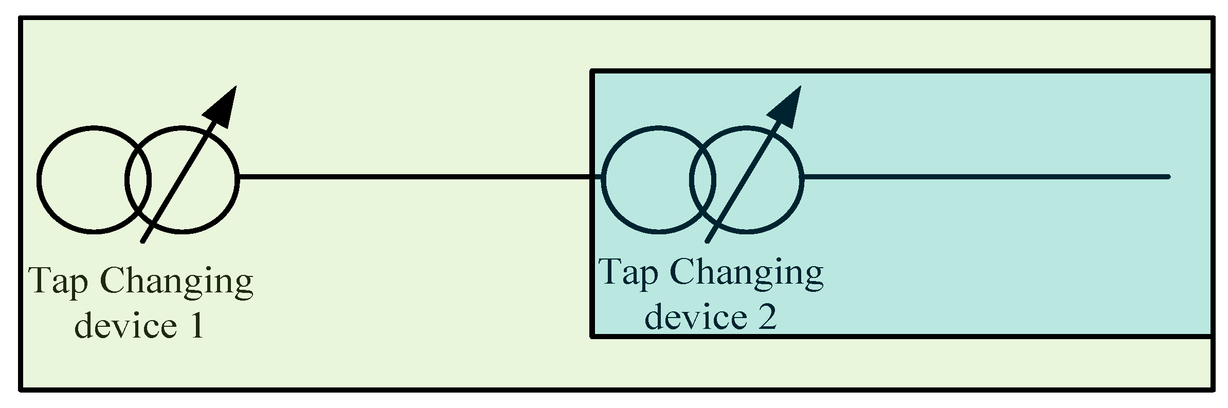
Tap changing deviceOLTC(−8–8) tap (initial position: 0)
SVR(−16–16) tap (initial position: 0)
Distributed generationInitial condition 1Active power: 0.5 MW, reactive power: 0 MVAR
Initial condition 2Active power: 0.5 MW, reactive power: 0.5 MVAR
Reactive power range−1.0–1.0 MVAR
Table 2. Continuous control reference for CVR of initial condition 1.
Voltage Control DeviceControl Reference
Tap changing deviceOLTC−0.8108
SVR1.9949
Reactive power deviceDG11.0
DG2−1.0
DG31.0
Objective function index199.9426
Table 3. Final control reference for CVR of initial condition 1.
Voltage Control DeviceControl Reference
Tap changing deviceOLTC−1
SVR2
Reactive power deviceDG11.0
DG2−0.2579
DG31.0
Objective function index212.1651
Table 4. Final control reference for CVR of initial condition 2.
Voltage Control DeviceControl Reference
Tap changing deviceOLTC−1
SVR2
Reactive power deviceDG11.0
DG2−0.7524
DG31.0
Objective function index190.2078
Table 5. Global optimum reference for CVR.
Voltage Control DeviceControl Reference
Tap changing deviceOLTC−1
SVR2
Reactive power deviceDG11.0
DG2−0.7063
DG31.0
Objective function index187.0994
Table 6. Comparison results of global optimum and initial condition.
ObjectiveDG1DG2DG3OLTCSVRObjective Function Index
Proposed method
(initial condition 1)
1.0−0.25791.0−12212.1651
Proposed method
(initial condition 2)
1.0−0.75241.0−12190.2078
Global optimum1.0−0.70631.0−12187.0994
Table 7. Continuous reference for nominal voltage of initial condition 1.
Voltage Control DeviceControl Reference
Tap changing deviceOLTC2.0697
SVR4.5818
Reactive power deviceDG11.0
DG20.3138
DG31.0
Objective function index30.8997
Table 8. Final control reference for nominal voltage of initial condition 1.
Voltage Control DeviceControl Reference
Tap changing deviceOLTC2
SVR5
Reactive power deviceDG11.0
DG20.3106
DG31.0
Objective function index32.0761
Table 9. Final reference for nominal voltage of initial condition 2.
Voltage Control DeviceControl Reference
Tap changing deviceOLTC2
SVR4
Reactive power deviceDG11.0
DG20.5109
DG31.0
Objective function index29.6959
Table 10. Global optimum reference for nominal voltage.
Voltage Control DeviceControl Reference
Tap changing deviceOLTC2
SVR4
Reactive power deviceDG11.0
DG20.2195
DG31.0
Objective function index25.5613
Table 11. Comparison of global optimum and initial condition results.
ObjectiveDG1DG2DG3OLTCSVRObjective Function Index
Proposal method
(initial condition 1)
1.00.31061.02532.0761
Proposal method
(initial condition 2)
1.00.51091.02429.6959
Global optimum1.00.21951.02425.5613
Table 12. System configuration of case study 2.
CompositionDescription
LoadTotal active power: 3801.89 kW
Total reactive power: 2694.10 kVar
Tap changing deviceOLTC(−8–8) tap (initial position: 0)
SVR(−16–16) tap (initial position: 0)
Distributed generationInitial condition 1Active power: 0.5 MW, reactive power: 0 MVAR
Initial condition 2Active power: 0.5 MW, reactive power: 0.5 MVAR
Reactive power range−1.0–1.0 MVAR
Table 13. Comparison results of global optimum and initial condition.
ObjectiveDG1DG2DG3OLTCSVRObjective Function Index
Proposed method
(initial condition 1)
0.37830.71171.0−4390.1840
Proposed method
(initial condition 2)
0.35180.69820.9683−4387.6787
Global optimum0.31430.87210.8311−4386.7507
Table 14. Comparison of global optimum and initial condition results.
ObjectiveDG1DG2DG3OLTCSVRObjective Function Index
Proposal method
(initial condition 1)
0.54361.01.00121.2980
Proposal method
(initial condition 2)
0.57691.01.00121.2162
Global optimum0.61201.01.00121.1830

