Experimental and Numerical Analysis of the Effect of Vortex Generator Height on Vortex Characteristics and Airfoil Aerodynamic Performance


Abstract
1. Introduction
2. Methods
2.1. Numerical Conditions
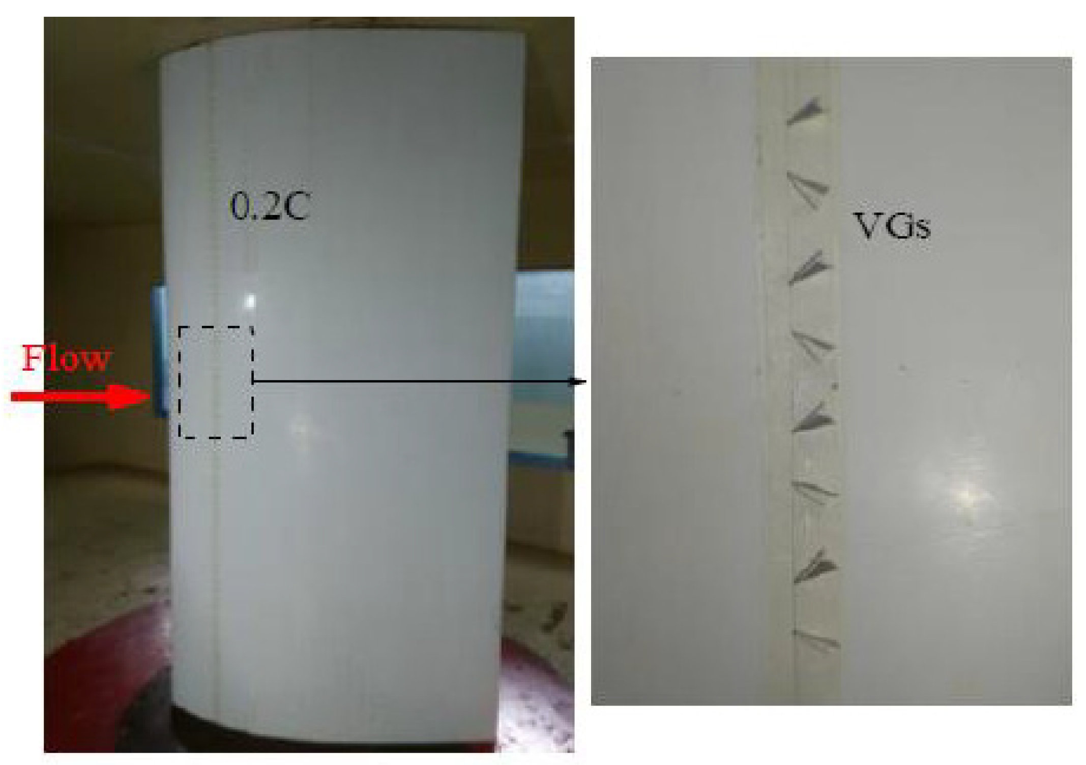
2.2. Experiment Setup
3. Results and Discussion
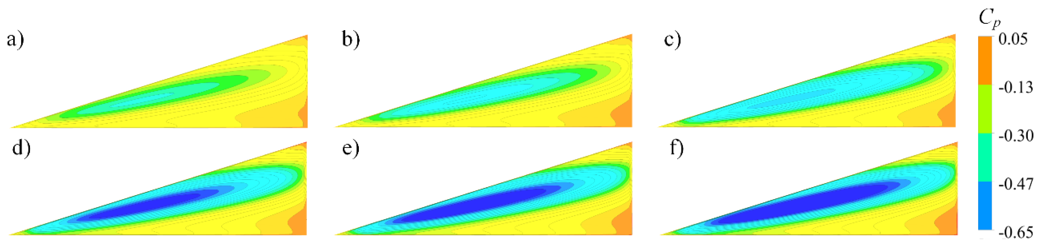
3.1. Analysis of CFD Calculation Results
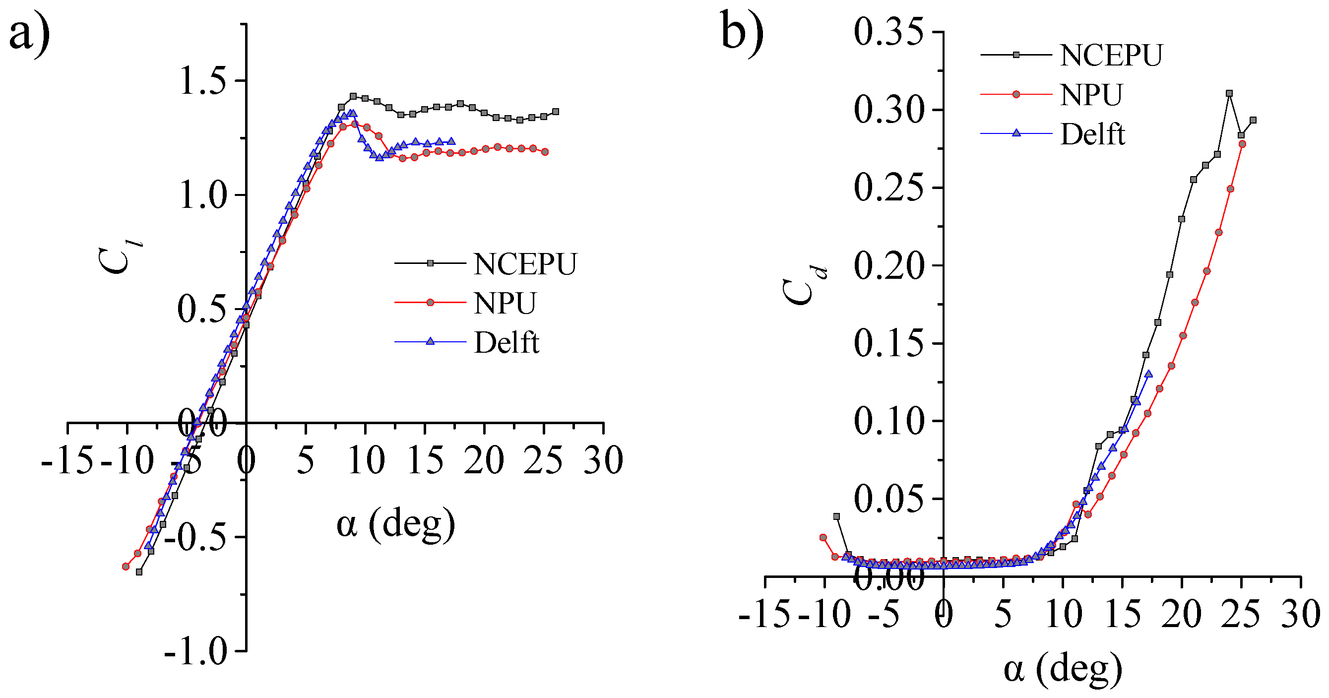
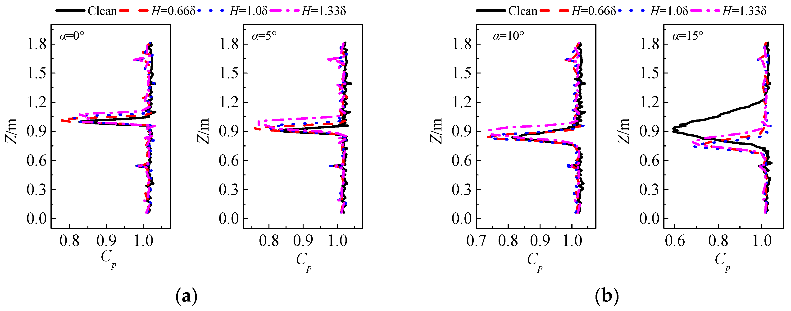
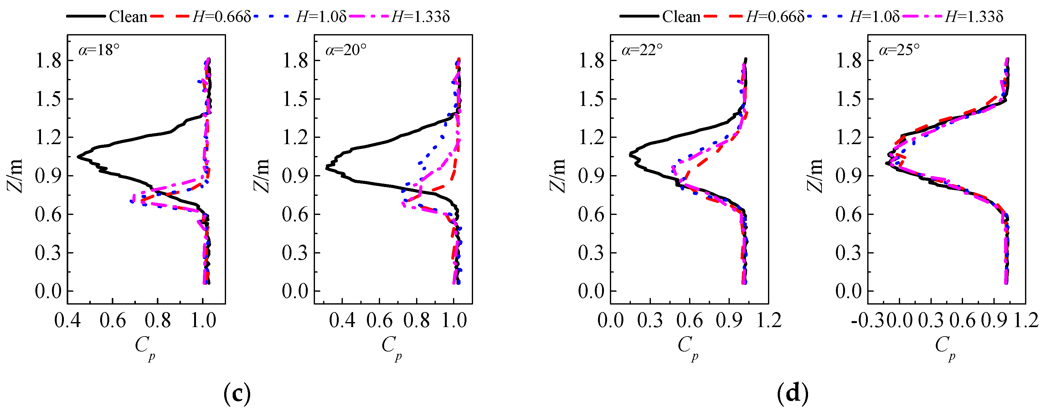
3.2. Analysis of Experimental Results
4. Conclusions
Author Contributions
Funding
Conflicts of Interest
References
- Council GWE. GWEC Global Wind Report 2017; Global Wind Energy Council: Bonn, Germany, 2017. [Google Scholar]
- Khamlaj, T.A.; Rumpfkeil, M.P. Analysis and optimization of ducted wind turbines. Energy 2018, 162, 1234–1252. [Google Scholar] [CrossRef]
- Wang, Y.; Li, G.; Shen, S.; Huang, D.; Zheng, Z.C. Influence of an off-surface small structure on the flow control effect on horizontal axis wind turbine at different relative inflow angles. Energy 2018, 160, 101–121. [Google Scholar] [CrossRef]
- Ebrahimi, A.; Movahhedi, M. Wind turbine power improvement utilizing passive flow control with microtab. Energy 2018, 150, 575–582. [Google Scholar] [CrossRef]
- Moshfeghi, M.; Shams, S.; Hur, N. Aerodynamic performance enhancement analysis of horizontal axis wind turbines using a passive flow control method via split blade. J. Wind Eng. Ind. Aerodyn. 2017, 167, 148–159. [Google Scholar] [CrossRef]
- Ebrahimi, A.; Movahhedi, M. Power improvement of NREL 5-MW wind turbine using multi-DBD plasma actuators. Energy Convers. Manag. 2017, 146, 96–106. [Google Scholar] [CrossRef]
- Lin, J.C. Review of research on low-profile vortex generators to control boundary-layer separation. Prog. Aerosp. Sci. 2002, 38, 389–420. [Google Scholar] [CrossRef]
- Macquart, T.; Maheri, A.; Busawon, K. Microtab dynamic modelling for wind turbine blade load rejection. Renew. Energy 2014, 64, 144–152. [Google Scholar] [CrossRef]
- Kametani, Y.; Fukagata, K.; Orlu, R.; Schlatter, P. Effect of uniform blowing/suction in a turbulent boundary layer at moderate Reynolds number. Int. J. Heat Fluid Flow 2015, 55, 132–142. [Google Scholar] [CrossRef]
- Ziadé, P.; Feero, M.A.; Sullivan, P.E. A numerical study on the influence of cavity shape on synthetic jet performance. Int. J. Heat Fluid Flow 2018, 74, 187–197. [Google Scholar] [CrossRef]
- Yang, H.; Jiang, L.-Y.; Hu, K.-X.; Peng, J. Numerical study of the surfactant-covered falling film flowing down a flexible wall. Eur. J. Mech. Fluids 2018, 72, 422–431. [Google Scholar] [CrossRef]
- Abdollahzadeh, M.; Pascoa, J.C.; Oliveira, P.J. Comparison of DBD plasma actuators flow control authority in different modes of actuation. Aerospace Sci. Technol. 2018, 78, 183–196. [Google Scholar] [CrossRef]
- Barlas, T.K.; van Kuik, G.A.M. Review of state of the art in smart rotor control research for wind turbines. Prog. Aerospace Sci. 2010, 46, 1–27. [Google Scholar] [CrossRef]
- Johnson, S.J.; Baker, J.P.; Dam, C.P.V. An overview of active load control techniques for wind turbines with an emphasis on microtabs. Wind Energy 2010, 13, 239–253. [Google Scholar] [CrossRef]
- Wang, H.; Zhang, B.; Qiu, Q.; Xu, X. Flow control on the NREL S809 wind turbine airfoil using vortex generators. Energy 2017, 118, 1210–1221. [Google Scholar] [CrossRef]
- Taylor, H.D. The Elimination of Diffuser Separation by Vortex Generators; United Aircraft Corporation: Moscow, Russia, 1947. [Google Scholar]
- Manolesos, M.; Voutsinas, S.G. Experimental investigation of the flow past passive vortex generators on an airfoil experiencing three-dimensional separation. J. Wind Eng. Ind. Aerodyn. 2015, 142, 130–148. [Google Scholar] [CrossRef]
- Gao, L.; Zhang, H.; Yongqian, L.; Han, S. Effects of vortex generators on a blunt trailing-edge airfoil for wind turbines. Renew. Energy 2015, 76, 303–311. [Google Scholar] [CrossRef]
- Afjeh, A.A.; Keith, T.G.; Fateh, A. Predicted aerodynamic performance of a horizontal-axis wind turbine equipped with vortex generators. J. Wind Eng. Ind. Aerodyn. 1990, 33, 515–529. [Google Scholar] [CrossRef]
- Hu, J.; Wang, R.; Huang, D. Flow control mechanisms of a combined approach using blade slot and vortex generator in compressor cascade. Aerosp. Sci. Technol. 2018, 78, 320–331. [Google Scholar] [CrossRef]
- Grébert, A.; Bodart, J.; Jamme, S.; Laurent, J. Simulations of shock wave/turbulent boundary layer interaction with upstream micro vortex generators. Int. J. Heat Fluid Flow 2018, 72, 73–85. [Google Scholar] [CrossRef]
- Urkiola, A.; Fernandez-Gamiz, U.; Errasti, I.; Zulueta, E. Computational characterization of the vortex generated by a Vortex Generator on a flat plate for different vane angles. Aerosp. Sci. Technol. 2017, 65, 18–25. [Google Scholar] [CrossRef]
- Oneissi, M.; Habchi, C.; Russeil, S.; Lemenand, T.; Bougeard, D. Heat transfer enhancement of inclined projected winglet pair vortex generators with protrusions. Int. J. Therm. Sci. 2018, 134, 541–551. [Google Scholar] [CrossRef]
- Mondal, B.; Lopez, C.F.; Verma, A.; Mukherjee, P.P. Vortex generators for active thermal management in lithium-ion battery systems. Int. J. Heat Mass Trans. 2018, 124, 800–815. [Google Scholar] [CrossRef]
- Godard, G.; Stanislas, M. Control of a decelerating boundary layer. Part 1: Optimization of passive vortex generators. Aerosp. Technol. 2006, 10, 181–191. [Google Scholar] [CrossRef]
- Godard, G.; Stanislas, M. Control of a decelerating boundary layer. Part 2: Optimization of slotted jets vortex generators. Aerosp. Sci. Technol. 2006, 10, 394–400. [Google Scholar] [CrossRef]
- Godard, G.; Stanislas, M. Control of a decelerating boundary layer. Part 3: Optimization of round jets vortex generators. Aerosp. Sci. Technol. 2006, 10, 455–464. [Google Scholar] [CrossRef]
- Velte, C.M. Characterization of Vortex Generator Induced Flow; Technical University of Denmark: Copenhagen, Denmark, 2009. [Google Scholar]
- Angele, K.P.; Grewe, F. Instantaneous Behavior of Streamwise Vortices for Turbulent Boundary Layer Separation Control. J. Fluid. Eng. 2007, 129, 226–235. [Google Scholar] [CrossRef]
- Sørensen, N.N.; Zahle, F.; Bak, C.; Vronsky, T. Prediction of the Effect of Vortex Generators on Airfoil Performance. J. Phys. Conf. Ser. 2014, 524, 12–19. [Google Scholar] [CrossRef]
- Mueller-Vahl, H.P.G.; Nayeri, C.N.; Paschereit, C.O. Vortex generators for wind turbine blades: A combined wind tunnel and wind turbine parametric study. In Proceedings of the ASME Turbo Expo 2012: Turbine Technical Conference and Exposition, Copenhagen, Denmark, 11–15 June 2012; pp. 899–914. [Google Scholar]
- Fouatih, O.M.; Medale, M.; Imine, O.; Imine, B. Design optimization of the aerodynamic passive flow control on NACA 4415 airfoil using vortex generators. Eur. J. Mech. Fluids 2016, 56, 82–96. [Google Scholar] [CrossRef]
- Velte, C.M.; Hansen, M.O.L. Investigation of flow behind vortex generators by stereo particle image velocimetry on a thick airfoil near stall. Wind Energy 2013, 16, 775–785. [Google Scholar] [CrossRef]
- Hansen, M.O.L.; Velte, C.M.; Øye, S.; Hansen, R.; Sorensen, N.N.; Mikkelsen, R. Aerodynamically shaped vortex generators. Wind Energy 2016, 19, 563–567. [Google Scholar] [CrossRef]
- Kerho, M.; Hutcherson, S.; Blackwelder, R.F.; Liebeck, R.H. Vortex generators used to control laminar separation bubbles. J. Aircr. 1993, 30, 315–319. [Google Scholar] [CrossRef]
- Timmer, W.A.; van Rooij, R.P.J.O.M. Summary of the Delft University Wind Turbine Dedicated Airfoils. J. Sol. Energy Eng. 2003, 125, 11–21. [Google Scholar] [CrossRef]
- Gyatt, G.W. Development and Testing of Vortex Generators for Small Horizontal Axis Wind Turbines; AeroVironment Inc.: Monrovia, CA, USA, 1986. [Google Scholar]
- Sullivan, T.L. Effect of vortex generators on the power conversion performance and structural dynamic loads of the Mod-2 wind turbine. A.V. Samokhvalov / Physica C 1984, 259, 337–348. [Google Scholar]
- Kogaki, T.; Matsumiya, H.; Kieda, K.; Yoshimizu, N. Performance Improvement of Airfoil for Wind Turbines by the Modified Vortex Generator. Wind Energy 2004, 28, 73–76. [Google Scholar]
- Fernandez-Gamiz, U.; Gomez-Mármol, M.; Chacón-Rebollo, T. Computational Modeling of Gurney Flaps and Microtabs by POD Method. Energies 2018, 11, 2091. [Google Scholar] [CrossRef]


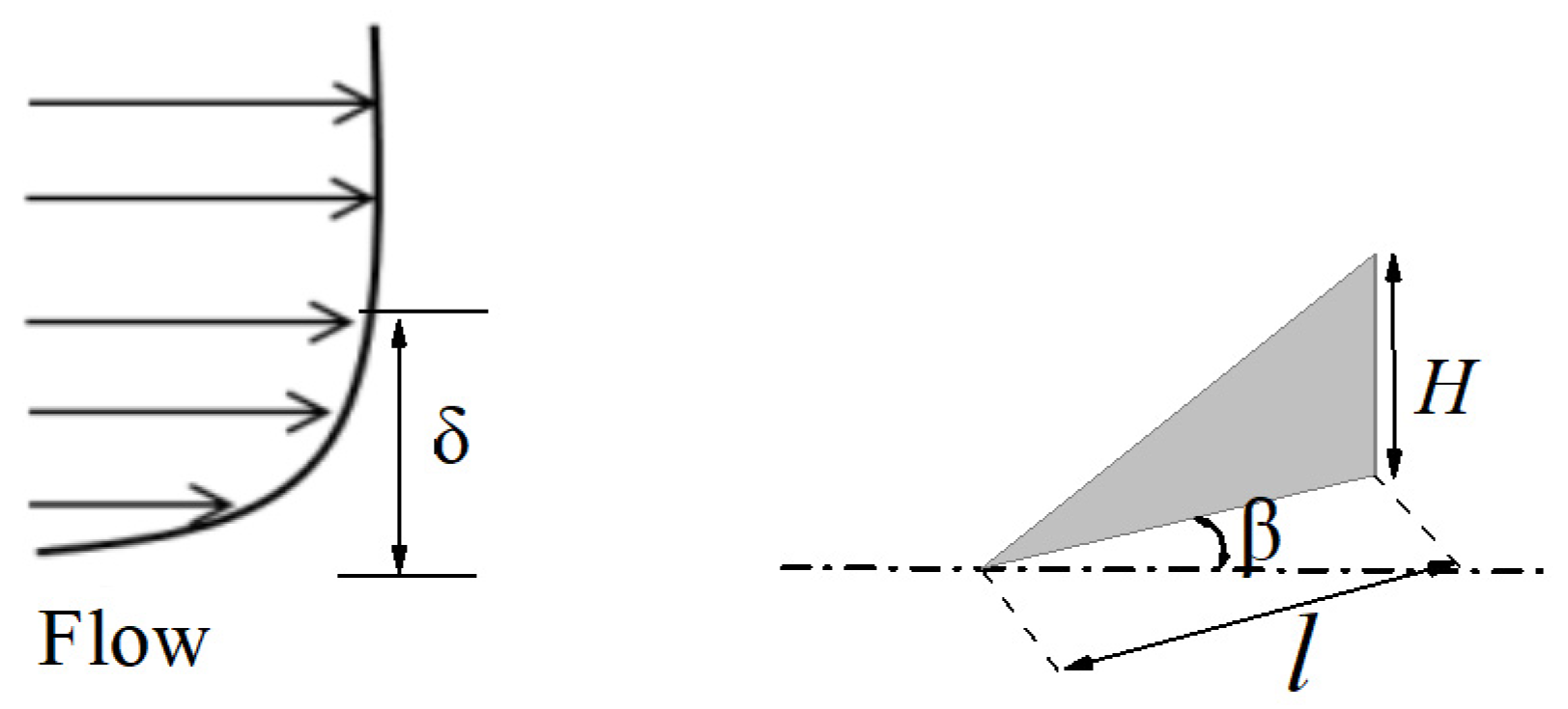
| Setting Angle β (°) | Length l (mm) | Hight H (mm) |
|---|---|---|
| 20 | 17 | 5 |
| Height Ratio | Case 1 | Case 2 | Case 3 | Case 4 | Case 5 | Case 6 |
|---|---|---|---|---|---|---|
| H/δ | 0.1 | 0.2 | 0.5 | 1.0 | 1.5 | 2.0 |
| H/δ * | 0.717 | 1.295 | 2.475 | 3.521 | 4.032 | 4.347 |
| H/θ | 1.03 | 2.083 | 5.15 | 10.416 | 15.479 | 20.661 |
| Variables | Mesh | Richardson Extrapolation | ||||
|---|---|---|---|---|---|---|
| Coarse | Medium | Fine | RE | p | R | |
| Cl | 0.5893 | 0.5918 | 0.5921 | 0.5922 | 3.05 | 0.12 |
| Cd | 0.2237 | 0.225 | 0.2251 | 0.2251 | 3.70 | 0.07 |
| Cl/Cd | 2.6211 | 2.6219 | 2.6221 | 2.6222 | 2.0 | 0.25 |
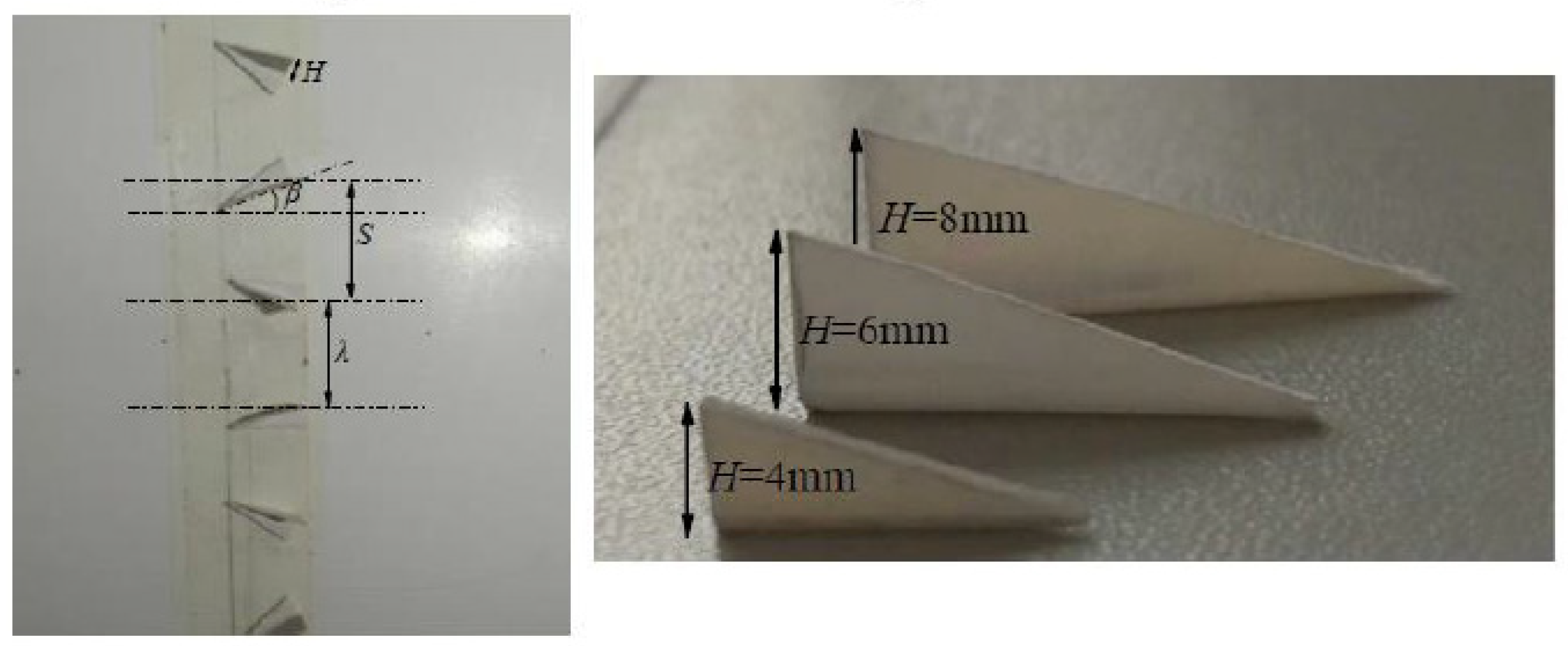
| Setting Angle β (°) | Length l/H | Hight H (mm) | Spacing S/H | Pitch Distance λ/H |
|---|---|---|---|---|
| 20 | 2.5 | 4, 6, 8 | 5 | 5 |
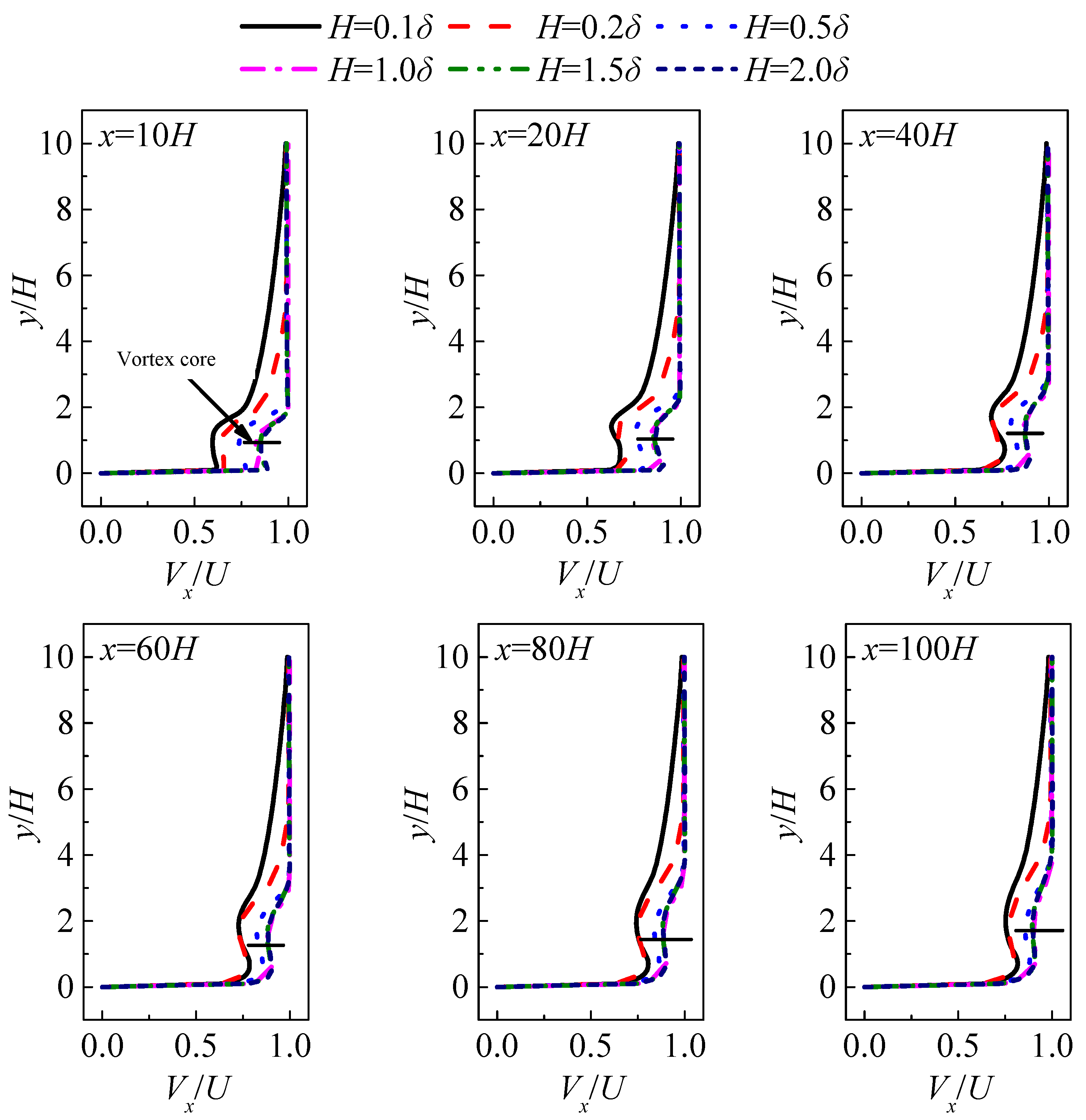
| Case | x = 10H | x = 20H | x = 40H | x = 60H | x = 80H | x = 100H |
|---|---|---|---|---|---|---|
| Clean | 0% | 0% | 0% | 0% | 0% | 0% |
| H = 0.1δ | 4.3% | 4.1% | 3.7% | 3.3% | 3.3% | 3.3% |
| H = 0.2δ | 8.7% | 4.5% | 3.7% | 3.3% | 3.3% | 3.3% |
| H = 0.5δ | 25.4% | 23.7% | 21.5% | 19.6% | 16.2% | 15.5% |
| H = 1.0δ | 34.1% | 32.8% | 31.1% | 28.4% | 25.5% | 24.6% |
| H = 1.5δ | 34.1% | 32.8% | 31.1% | 28.4% | 25.5% | 24.6% |
| H = 2.0δ | 34.1% | 32.8% | 31.1% | 28.4% | 25.5% | 24.6% |
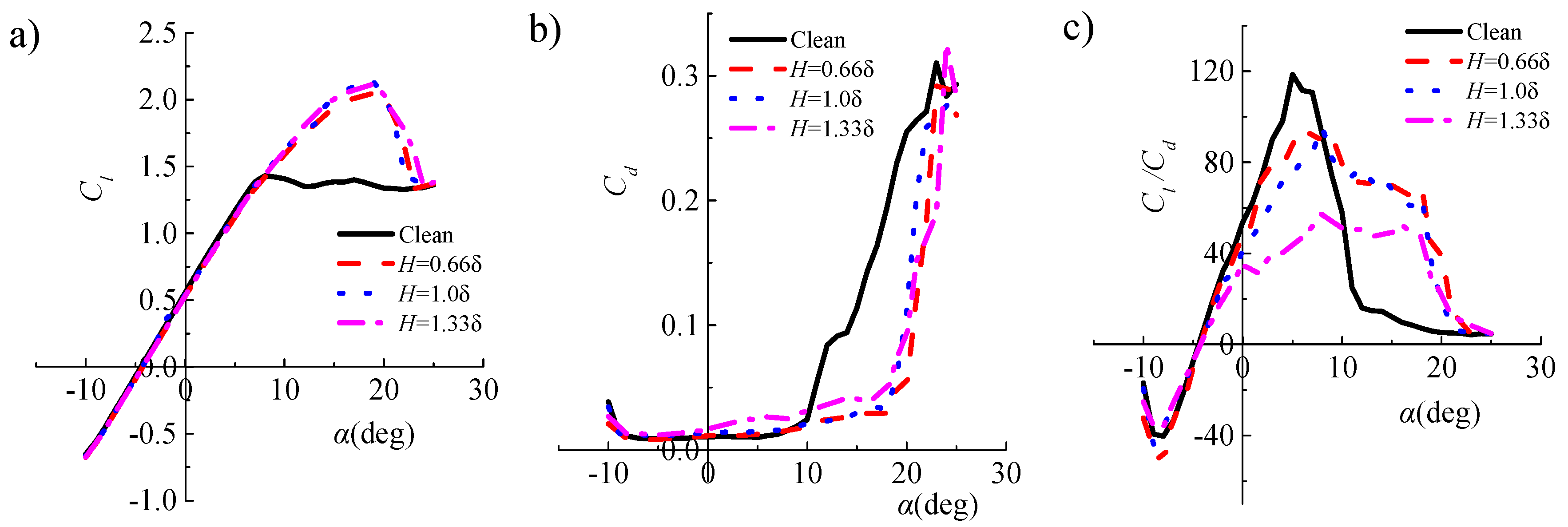
| Case | Stall Attack Angle | Increment of Maximum Cl | Decrease of Cd at 18° | Decrease of Maximum Lift–Drag Ratio | Increment of Lift–Drag Ratio at 18° |
|---|---|---|---|---|---|
| Clean | 8° | 0% | 0% | 0% | 0% |
| H = 0.66δ | 18° | 42.8% | 84.9% | 19.7% | 880.3% |
| H = 1.0δ | 18° | 48.7% | 83.2% | 19.3% | 821.8% |
| H = 1.33δ | 18° | 48.6% | 76.8% | 51.2% | 564.8% |
© 2019 by the authors. Licensee MDPI, Basel, Switzerland. This article is an open access article distributed under the terms and conditions of the Creative Commons Attribution (CC BY) license (http://creativecommons.org/licenses/by/4.0/).
Share and Cite
Li, X.; Yang, K.; Wang, X. Experimental and Numerical Analysis of the Effect of Vortex Generator Height on Vortex Characteristics and Airfoil Aerodynamic Performance. Energies 2019, 12, 959. https://doi.org/10.3390/en12050959
Li X, Yang K, Wang X. Experimental and Numerical Analysis of the Effect of Vortex Generator Height on Vortex Characteristics and Airfoil Aerodynamic Performance. Energies. 2019; 12(5):959. https://doi.org/10.3390/en12050959
Chicago/Turabian StyleLi, Xinkai, Ke Yang, and Xiaodong Wang. 2019. "Experimental and Numerical Analysis of the Effect of Vortex Generator Height on Vortex Characteristics and Airfoil Aerodynamic Performance" Energies 12, no. 5: 959. https://doi.org/10.3390/en12050959
APA StyleLi, X., Yang, K., & Wang, X. (2019). Experimental and Numerical Analysis of the Effect of Vortex Generator Height on Vortex Characteristics and Airfoil Aerodynamic Performance. Energies, 12(5), 959. https://doi.org/10.3390/en12050959