1. Introduction
Metal Oxide Varistors (MOVs) are the newest and most advanced category of surge protectors due to their obvious advantages. MOVs are manufactured in an extremely wide range, as protective equipment for each voltage level, from telecommunication networks and low voltage electrical installations to high and very high voltage, regardless of the current type (AC or DC). Nowadays, there are studies on the implementation of these varistors, even in the field of power electronics, as protection elements for power semiconductor devices operating under forced commutation [
1].
Although the research on non-linear properties of semiconductor ceramics based on metal oxide mixtures dates back to the 1950s and was carried out in Japan and the former Soviet Union, the first patent in this field, owned by the Japanese company Matsushita Electric Industrial Co., was granted in 1968 [
2] and these pieces of equipment first appeared on the market in the early 1970s. Most of the giant companies in the electrotechnical field have included in their manufacturing programs such equipment, especially for medium and high voltage fields. In low-voltage and telecommunications, small and medium-sized companies are predominant, equipment in this area not being highly demanding as manufacturing technology. We will not detail the existing technical solutions along the way [
3].
The development of overvoltage protection equipment using metal oxide based varistor is a direct consequence of the main global concerns in order to improve the quality and continuity of power supply services, increase safety in the operation of electrical networks, and meet the requirements of specific categories of electricity users [
4].
Low-voltage protection equipment using Metal Oxide Varistors (ZnO-based varistors) consists of compact protection modules, some of them in combination with gas discharge tubes (GDT) and various types of diodes or fuses [
5]. A single low-voltage varistor cannot respond simultaneously to the following requirements:
Have a transitory level of protection as close as possible to the service voltage;
Withstand temporary temporal overvoltage in relation to each other;
Maintain constant its threshold voltage over time, avoiding "aging";
Do not come into thermal runaway after an extremely violent impulse, being further fed to the rated voltage of the grid. Instead, it has a very low reaction time of up to 25 ns
There is a huge risk of overheating, especially after an impulse, because of the constant current flow, the relatively low mass and limitations of heat dissipation possibilities, since it also operates in the weakly non-linear region of the characteristic parameters. The varistor may enter a transient violent process (impulses of voltage) in thermal runaway mode. From an electrical point of view, this state is manifested by the tendency of the varistor to provide a minimum impedance path (resistance), after the passage of the overvoltage wave, having low electrical resistance due to its high temperature, (the network being thus grounded in an unwanted short circuit) [
6].
In most overvoltage protection devices, heat is constantly developing by the transformation of a significant part of the electromagnetic energy into thermal energy, even when surge waves are not applied at their terminals due to the fact that ZnO-based varistors are crossed at nominal voltage, by a certain electrical current. As a result, the heat generated in the varistor, the temperatures of various parts or equipment increase to the limit temperatures corresponding to the stationary regime when all heat is released to the environment.
The equipment, in steady state, possesses a certain calorific load, which is kept in a potential state. This would be lost through progressive dissipation in the colder environment only in the event of disconnection of the equipment from the grid. The value of this latent heat represents only a fraction of the value of the electric energy that turns into heat inside the varistor, through the effect of Joule-Lenz in the event of a surge wave [
7].
In the case of applying an overvoltage impulse, which leads to the occurrence of an important overcurrent, this state of stationary thermal equilibrium is exceeded. In order to guarantee the exemplary and long-lasting operation of the protective equipment, in terms of thermal stresses, the manufacturing standards require (subject to the materials used and the operating conditions) certain maximum permissible limits for stationary temperature.
There is a problem of the mathematical modeling of the temperature field during impulse application, due to the very large variation of the parameters involved. As a result, we can only take into account the global increase in varistor temperature after passing the impulse current wave.
Essentially, the passage of the impulse current wave with the conversion of electrical energy into heat through the Joule-Lenz effect is a purely adiabatic process [
8]. Due to the extremely low impulse duration (less than 1 ms), the varistor does not give up heat to the environment either through convection or radiation. The only possibility of rapid heat dissipation, during the impulse, and especially in the next few seconds, is conduction. The heat is thus conveyed via the varistor connections.
We noticed that the whole energy of the impulse accumulates in the form of heat in the mass of the varistor, which inevitably leads to an increase in its temperature [
9]. This heat must then be discharged from the varistor mass as, as we have shown above, the increase in varistor temperature favors the electrical conduction and leads to the thermal runaway with the well-known consequences.
Evacuation of this heat is achieved mainly by convection and to a lesser extent through radiation and conduction.
It is very useful that, in order to ensure an optimal design of overvoltage protection equipment, to be aware of the measures that can be taken to avoid the risk of thermal varistor overheating in the service mode that is established after the application of the impulse. As a result, we can speak of the thermal stability of the varistor in two cases [
10]:
Both situations will be analyzed. When the varistor passes the high voltage impulse wave,
W, the process being adiabatic, the whole energy
Q =
W, dissipated by Joule effect, remains stored in the mass of the varistor, producing the temperature increase, Δ
θ1. It is desirable that this increase does not lead to the exceedance of the equilibrium temperature limit [
11].
The expression of the temperature increase of the varistor as a result of heat accumulation
Q is:
where
mv is the mass of the varistor and
cv is its specific mass heat.
The energy of the impulse, recovered in the total stored heat Q, of course, cannot be reduced, being a parameter that is related to external demands. On the contrary, it is quite desirable for the equipment to withstand the highest energy impulses.
The specific heat of the varistor
cv is a parameter that cannot be spectacularly interfered with. It is a parameter that results from the manufacturing technology and must be accepted as such, especially as the main objective of the manufacturer is to improve the non-linearity of the
I(
U) characteristic, the objective of which is subject to its whole approach. In addition, this issue of matter chemistry and physics is not the object of the varistor user’s concerns (the manufacturer of surge protectors) [
12].
The increase of the
mv varistor mass is achievable within the limits imposed by the electrical parameters, knowing that the height of the varistor is fixed by the voltage level at which it operates. By consequent, the only viable solution would be to increase the diameter, within the limits imposed by the standards. The solution is not always economically justified (the cost price of a disc varistor increases with its diameter and type) nor does it bring significant improvements, the heat remaining stored in the active mass of the varistor [
12].
2. Parallel Connection of Varistors
A first technical solution proposed by the authors is the parallel installation of two varistors instead of one. The solution is seemingly trivial and economically unjustified. But the essence of the proposed solution consists in the thermal coupling of the two varistors by thermal conduction, which would lead to the equalization of the temperatures of the two varistors and would lead to the forced limitation of the currents by the varistors.
Equation (1) is rewritten as:
If the masses of the two varistors are equal
mv1 =
mv2 and the specific heat
cv1 =
cv2, we obtain a half reduction of the temperature difference. The thermal coupling is essential because, in its absence, the varistor that has the lowest threshold voltage (if not identical) will take up most of the shock energy, overheating. The heat coupling attempts to force identical heating [
13].
The assembly behaves as though instead of the two varistors there was one, with a larger mass, without diminishing the choice of the level of protection [
14].
As we have seen before, the parallel connection of the varistors, together with their thermal coupling, is a technical solution designed to improve their thermal stability and, by consequence, the surge protection devices that embed them [
15]. Therefore, we will continue to present the results to proove this.
For this study, two varistors manufactured by the authors, according to an original technology, were used in the "Génie Electrique"—Laplace Laboratory of the Paul Sabatier University in Toulouse. All experimental determinations were also performed within the same laboratory. Varistors manufactured by the author were called R and S. The electrical characteristics I(U) of these varistors, determined in the cold state for currents between 0 and 10 mA, are almost similar.
The measured threshold voltages (at 1 mA) are:
It is noted that the two electrical characteristics, even if they are not identical, are close enough.
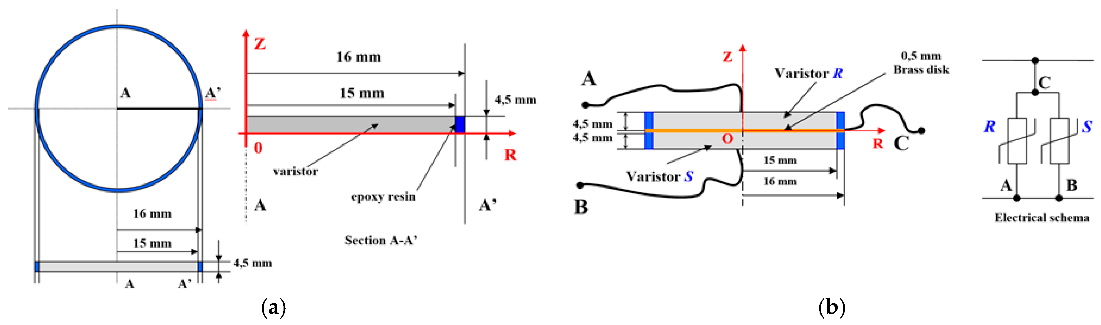
The dimensions of each of the varistors, in standalone position, are shown in
Figure 1a. This is the configuration in which varistors operate on their own, without thermal coupling or without additional brass masses.
The essence of this whole chapter is the thermal coupling of varistors mounted in parallel. The proposed technical solution consists in gluing the two varistors
R and
S, added to the faces of a 0.5 mm thick, disk-shaped brass sheet,
C with a diameter of 32 mm, which also plays the role of a common electrode. The parallel assembly is shown in
Figure 1b.
It was preferred to present the geometry of these varistors independently of the geometry of the others, given their specificity and the purpose for which they were achieved. Due to the cylindrical symmetry around the OZ axis, we find that the heat transfer modeling can be done only in section A-A’, the conclusions can be generalized by extrapolation. Moreover, from a mathematical point of view, modeling can only be performed on the upper half of section A-A’. We preferred modeling across the entire section for reasons of simplifying boundary conditions. The coordinate points, related to (0,0) were entered: (15,0); (16,0); (16,4.5); (15,4.5); (0,4.5).
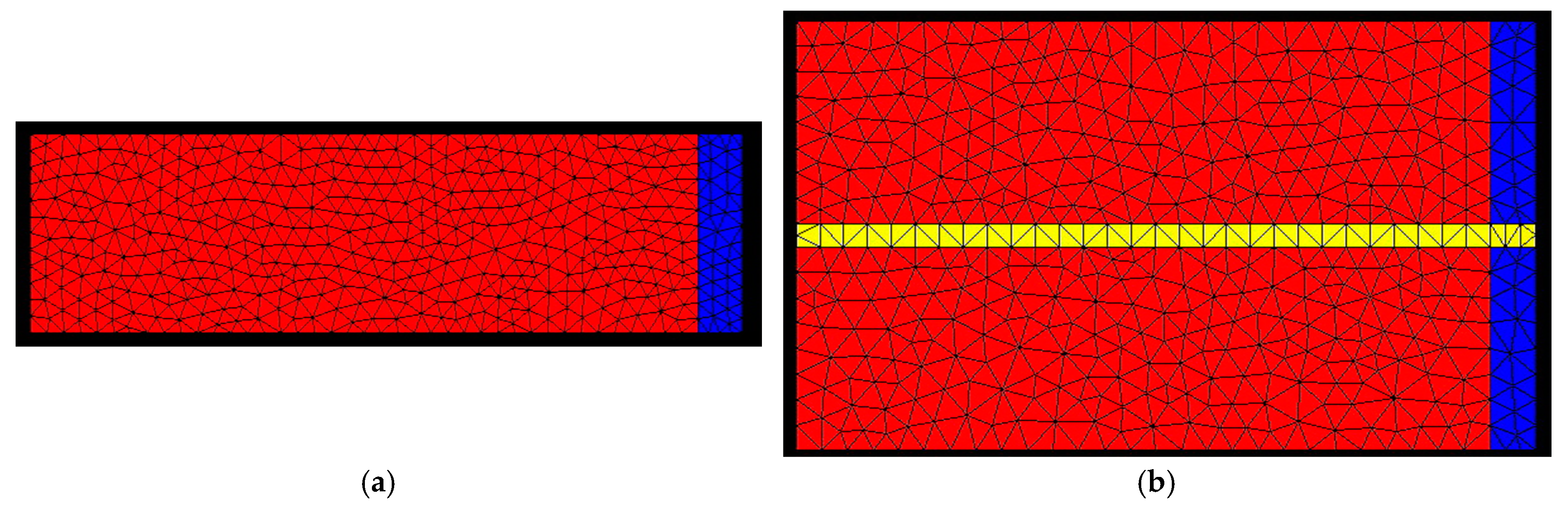
The mesh subdomains correspond to the materials (varistor—red, epoxy resin—blue). Border areas are the two sides of the varistor as well as the border between resin and air insulation, as shown in
Figure 2a,b. For modeling the heat transfer in case of both configurations, we used FLUX 2D, which is a dedicated finite elements-based software, suitable for this kind of complex applications, having cylindrical symmetry [
16].
Figure 2a presents the finite elements-based mesh for the standalone configuration and
Figure 2b presents the model for the parallel configuration, with the thermal brass coupling. The discretization of the section in
Figure 2a contains 1945 nodes, the finite elements being located as follows:
The discretization of the section in
Figure 2b contains 1932 nodes (no need for more elements because the accuracy is higher on such a small domain), the finite elements being located as follows:
Apparently, this structure has no advantage, since each of the two varistors has “lost” one of the faces, used as heat dissipation surfaces. Instead, the assembly behaves like a dual-mass varistor, but traversed by an approximately two-fold lower current [
17] (when an impulse is applied).
If the two I(U) characteristics are different (in the present case very little different) the currents that will pass through the varistors will be different, the varistor with the lower UN threshold voltage will withstand the higher current (and hence a higher heating). If this thermal coupling is achieved, the temperature of the two varistors will be forced as one, through the brass electrode.
This phenomenon is, actually, more complex, because in the case of the cold temperature varistor, we will also witness an increase in the current through it [
18]. If the difference between the threshold voltages of the two varistors is below 5%, we can safely say, (experimentally confirmed by the authors) that we are witnessing a forced equalization of the currents in a permanent regime, even if the varistors are exposed to the same voltage. The analysis of the thermal stability of both geometries will be performed:
Data obtained from modeling will be confronted with the experimental results. It is preferable to present in parallel the results of the modeling and the experimental results, in order to better highlight and compare them, without introducing an artificial barrier between the theoretical model and the physical reality.
3. Thermal Stability under Permanent Regime
The study involves two stages:
We will start by describing the experimental set-up.
3.1. Experimental Equipment for Permanent Regime Tests
All the experimental results described by the authors were obtained at the “Génie Electrique”—Laplace Laboratory of the Paul Sabatier University in Toulouse, France, by using the equipment located there.
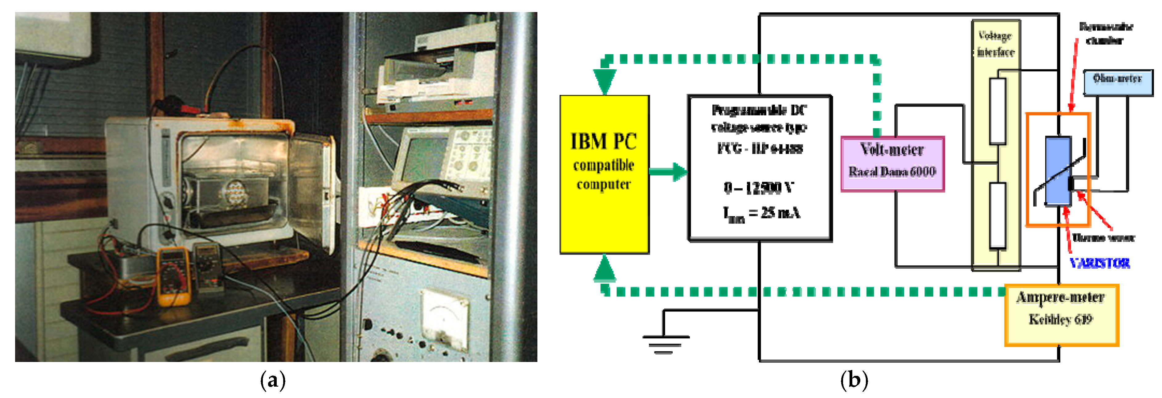
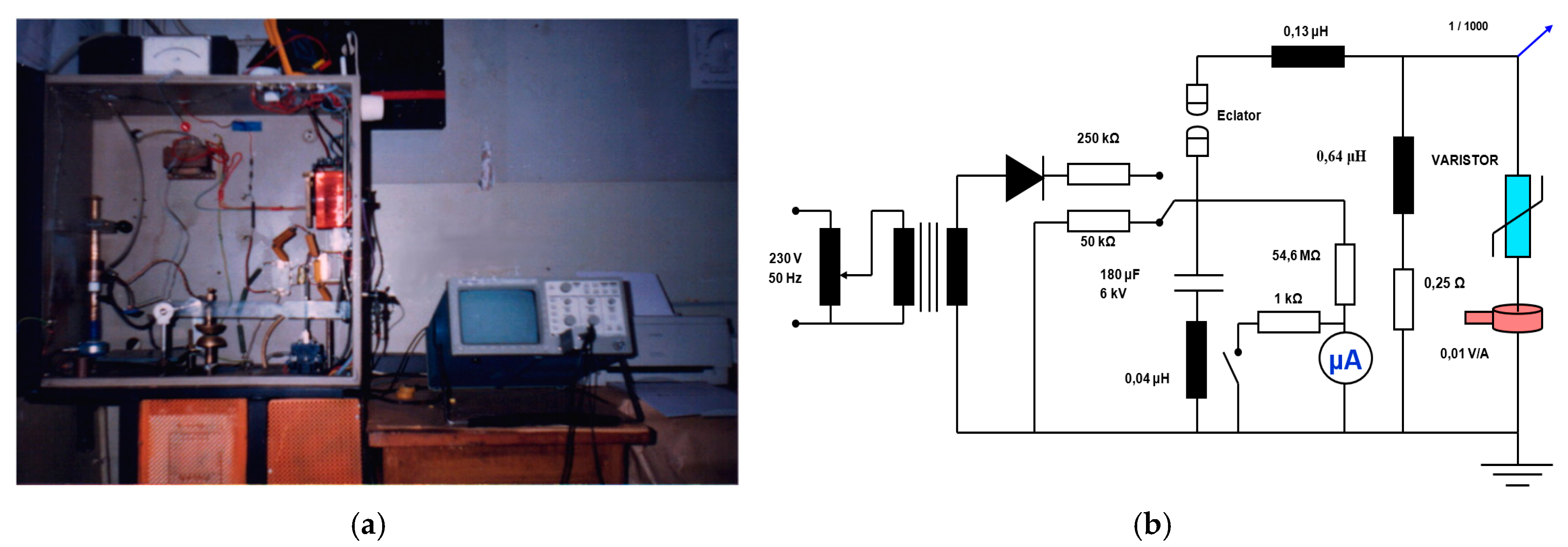
Figure 3a presents the general view of the equipment and
Figure 3b presents the electrical schema of this device. The elements of the electrical scheme as shown in
Figure 3b, are:
A continuous voltage source, programmable, type FUG-HP 64488, capable of delivering a continuous voltage between 0 and 12,500 V at a maximum current of 25 mA. The source can also be adjusted manually;
A digital electrometer, which allows the currents to be measured between 1.9 × 10⁻⁹ and 1.9 × 10⁻³ A, having a precision class of 0.5%;
A digital voltmeter, measuring the applied voltage between the varistor faces through a resistive divider with a ratio of 1:1000, having a precision class of 0.1%;
Two portable multimeters (only one of which is represented in the diagram) operating in ohmmeter mode, used to measure the resistance of the thermal sensors.
The varistor is connected by wires, not electrodes, to avoid their influence on the varistor. It is suspended vertically inside the oven to have the same thermal transmissivity on both sides. Two-point temperature measurements were made on symmetrical varistor sides, close to the axis of symmetry [
19]. As sensors, we used platinum ones, extremely sensitive in the temperature range from 20 °C to 100 °C, (Δ
R/
R > 1.5% for a Celsius degree). For measuring their electrical resistance, two standard digital multimeters (visible in the photo) were used. These thermoresistances have previously been calibrated by the manufacturer and checked in the laboratory.
As all tests will be done at ambient temperature, which is around 24 °C, the presence of an insulating box is not necessary. The samples to be analyzed are placed in a closed enclosure (the suspended metal box shown in the figure). Therefore, the influence of convection flow in the room is excluded. To have the same thermal transmittance value by convection
αC, on both sides, the samples are arranged vertically. The values of global thermal transmissivity (through convection and radiation) are, according to [
20]:
3.2. Analysis of Permanent Service Regime for A Single Varistor
In this first part we aim to achieve a numerical modeling of the temperature field in permanent mode in each of the two varistors, if they are not thermally coupled and operate independently.
The measurements shall be made at a voltage
U = 460 V, which corresponds to the operating coefficients at the stationary thermal stability limit [
21]:
C = 0.821 for R, and,
C = 0.83 for S,
where, C = U/UN, the ratio between the applied and the nominal voltage.
Following the measurements made, the values of the stationary currents were determined as:
The stationary power dissipation (P = U × I) will therefore be:
P = 0.303 W for R and,
P = 0.308 W for S.
The total heat dissipation area (the two sides + side surface) is:
It is noted that, practically, the two powers are equal, so only one of the varistors, for example
S, is enough to be considered. The estimated stationary over temperature regime
τse is, according to the formulas presented above (in °C):
We will consider that when the 3600 s passed from the connection of the varistor, its thermal transient heating regime is over, the varistor entering the permanent thermal regime.
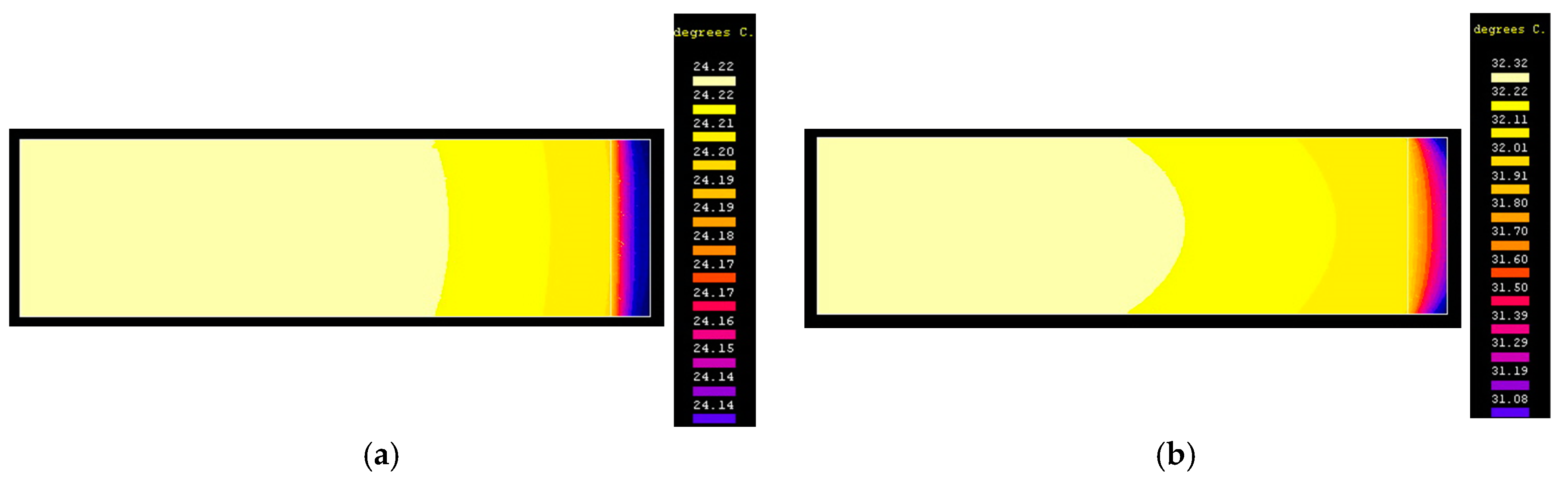
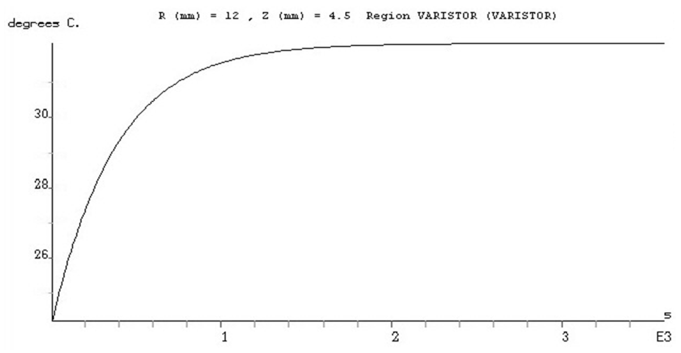
Figure 4a shows the distribution of the temperature field within the varistor at the passage of 10 s from the start of the heating process.
Figure 4b shows the distribution of the temperature field within the varistor at the passage of 3600 s from the start of the transient heating process, when the stationary regime was virtually reached.
It is noted that the highest temperature inside the varistor is approx. 32.32 °C and is obviously reached in the center of the varistor. The lowest temperature value is approx. 31.08 °C and is located at the edge of the epoxy resin insulation. It is noticeable that the difference between them is not spectacularly high, being at maximum 2 °C. The largest stationary overtemperature resulting from modeling is
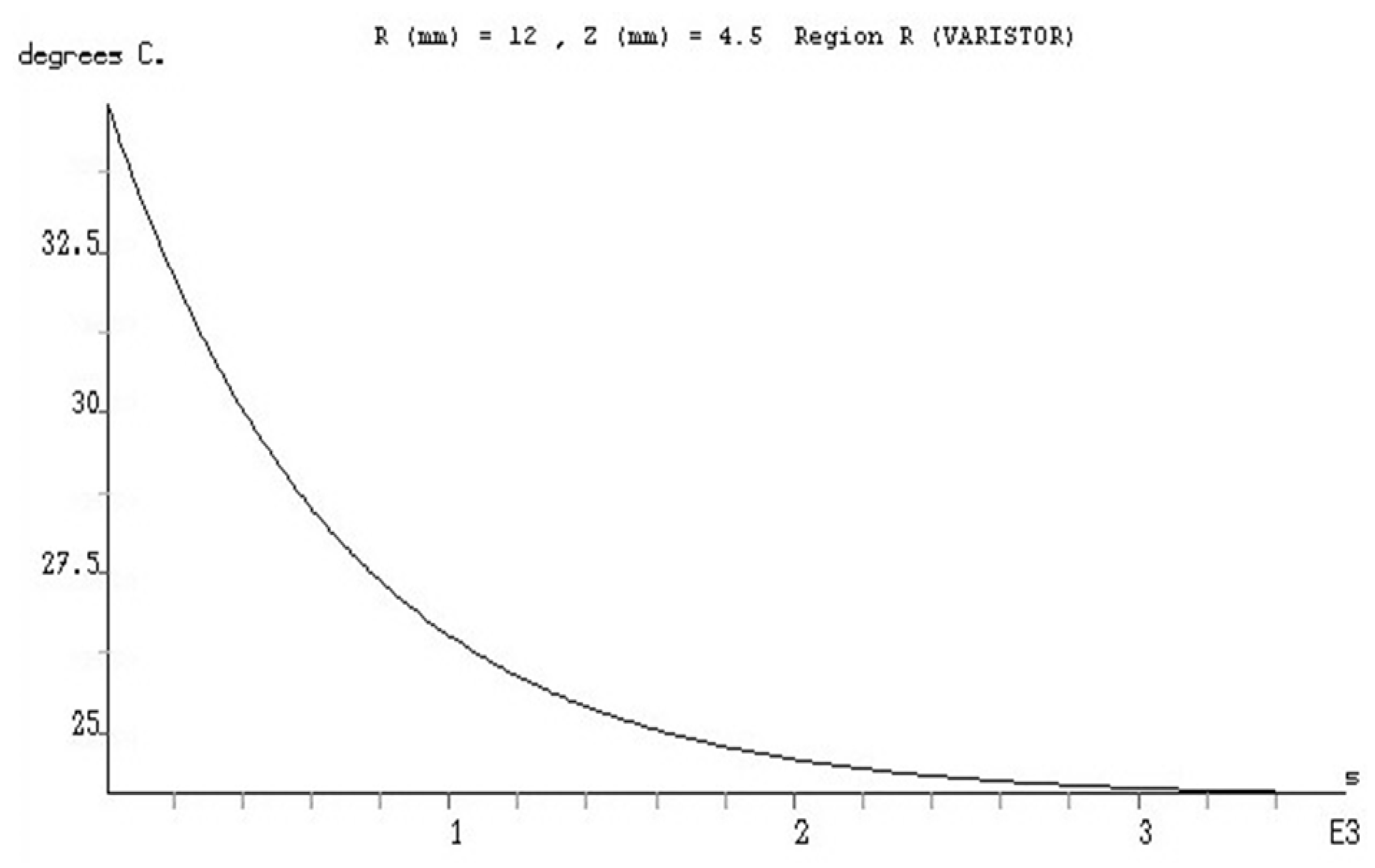
τsm = 8.32 °C. In order to be able to present the evolution of the temperature during the heating process, until we reach the stationary regime, we will consider a point on the upper surface of the varistor at
R = 12 mm and
Z = 4.5 mm. The time evolution of temperature at this point is shown in
Figure 5.
The graph above is provided by the FLUX 2D program. In the analysis of the stationary regime, we are less interested in the evolution of temperature over time, this being slightly different from the one presented in the previous graph, especially because of the variation of the varistor developed power, previously assumed to be constant. The developed power varies depending on the temperature due to the influence of the temperature on the current flowing through the varistor, which is initially with a smaller order than at the end of the process. This observation of the power variation developed is valid during the first 500–1000 s of the process. In
Table 1, we will present a comparison between the experimental data and the numerical model of thermal transfer:
We notice that the measured values are very close to those resulting from the modeling. These values are also close to the estimated value, given by Equation (3) as τse = 8.79. The difference between these temperatures may be caused by material inconsistency, measurement inaccuracy, thermal conduction in bonding wires, etc.
3.3. Analysis of Permanent Service Regime for the Two Varistors, in Parallel and Thermally Coupled
The total heat dissipation area for this case (the two sides + side surface) is Sl = 2.56 × 10⁻³ m2.
The estimated stationary over temperature regime
τse is, according to the formulas presented above (in °C):
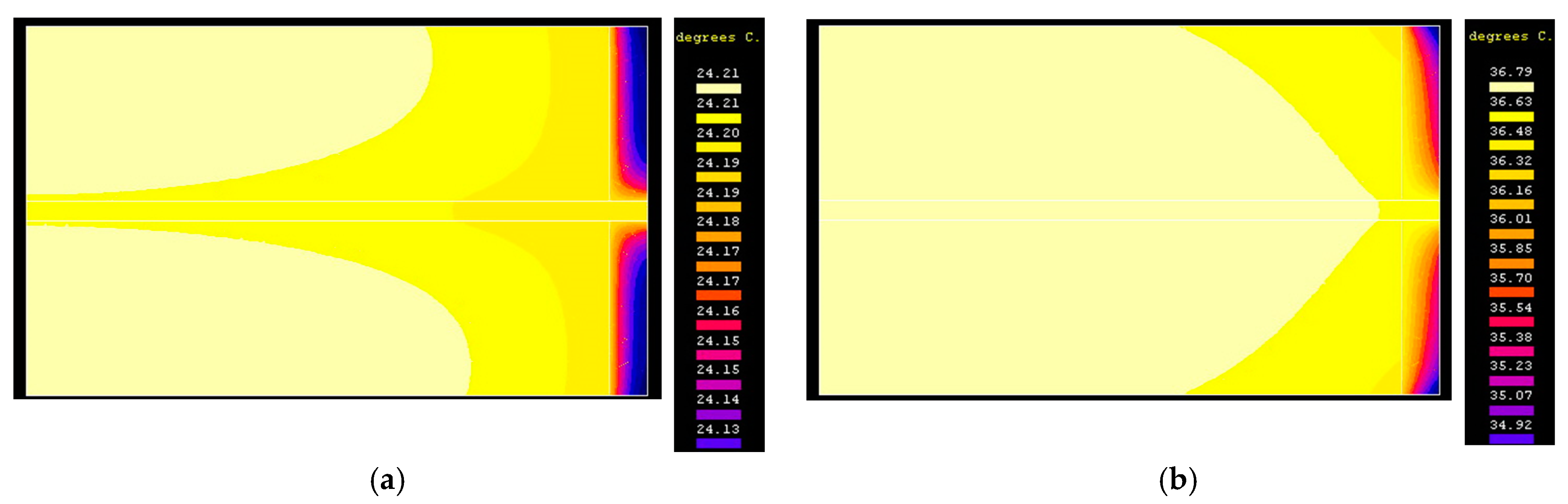
Figure 6a shows the distribution of the temperature field within the assembly at the passage of 10 s from the start of the heating process.
Figure 6b shows the distribution of the temperature field within the assembly at the passage of 3600 s from the start of the transient heating process, when the stationary regime was virtually reached.
We notice that the highest temperature inside the varistor is approx. 36.79 °C and is obviously reached in the central area of the varistor.
The lowest temperature value is approx. 34.92 °C and is located at the edge of the epoxy resin insulation. It is noticed that the difference between them is not spectacularly high in this case, being at maximum 2 °C.
The largest stationary over temperature resulting from modeling is
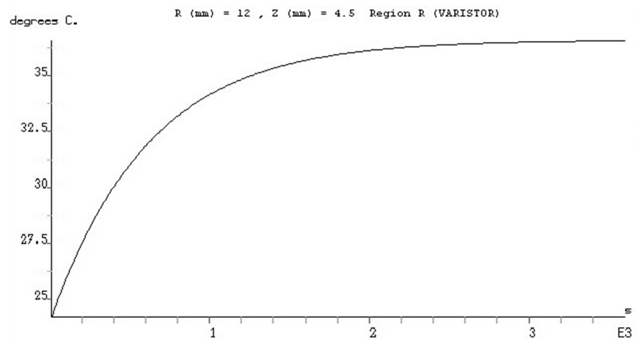
τsm = 12.79 °C. In order to be able to present the temperature evolution during the heating process, until reaching the stationary regime, we will consider a point on the upper surface of the varistor
R, located at
R = 12 mm and
Z = 4.5 mm, as in previous case of the varistor stand alone. The time evolution of temperature at this point is shown in
Figure 7.
In
Table 2, we will present a comparison between the experimental data and the numerical model of thermal transfer:
We notice that the measured values are very close to those resulting from the modeling. These values are also close to the estimated value, which is given by Equation (4) as τse = 13.9 °C. The difference between these temperatures can be caused by material inconsistency, measurement inaccuracy, thermal conduction in bonding wires, variation in material parameters, ambient temperature, etc.
4. Thermal Stability under Impulse Regime
As in previous case, this study involves two stages:
We will start by describing the experimental set-up for impulse tests.
4.1. Experimental Equipment for Impulse Regime Tests
Thermal stability analysis of ZnO-based varistors (and implicitly the equipment that embed them) needs to be done in an impulse mode, corresponding, mostly to lightning strokes. As we have mentioned in numerical modeling, the most unstated thermal regime is the one that is crossed by a varistor during and after the application of a relatively high voltage impulse.
These impulses were applied to the varistor without a prior polarization voltage (at nominal voltage), the varistor being initially heated at room temperature, i.e., at approx. 24 °C. In fact, the varistor remains polarized at the nominal voltage even after the overcurrent wave passes, but the influence of this polarization on the varistor temperature remains negligible, as in the permanent service regime, at the rated voltage of the network. Therefore, to study the evolution of the varistor over temperature during and after the application of an impulse, it is not necessary to polarize it in advance. There are standards that provide for such combined tests, which involve quite sophisticated installations [
22].
Figure 8a presents an overview of the impulse generator as installed at the “Génie Electrique”—Laplace Laboratory of Paul Sabatier University in Toulouse, France. The electrical schema of the impulse generator is shown in
Figure 8b.
The generator provides a bi-exponential impulse wave in current, type 8/20 μs, standardized according to IEC 60060-2. The voltage at which the 180 μF capacitor is charged (shown in
Figure 8b) is approximately 2000 V cc, the maximum voltage applied to the varistor being somewhat lower, between 1700 and 1900 V.
The simulation of impulse generator behavior was performed by the author using a custom and original dedicated program, "GIT-RE.exe". This program was designed in the Borland C language and it is not relevant for this article. The purpose of this program is to pre-estimate the maximum value of the voltage applied to the varistor, starting from the voltage at which the capacitor is charging. It provides an analytical estimation before applying the impulses.
The process happens in microseconds and can be considered adiabatic; the varistor has no time to evacuate the heat into the environment. The entire pulse energy remains stored in the varistor body, producing an extremely rapid temperature increase. The way in which the varistor or the varistor plus mass assembly is behaving in this situation is subject to other researches [
5].
The energy stored in the 180 μF capacitor in
Figure 8b, charged at 2000 V in our tests, is then applied to the varistor, causing its heating [
5]. We can safely say that the losses inside the test facility are negligible [
5]. The expression of this energy is given by the classic formula:
Using the above values of the parameters, we obtain an energy of approx. 360 J. Applying such an impulse to the varistor produces its heating. In order to capture exactly both the value and the waveform of the applied voltage, respectively the current set by the varistor, a simple digital oscilloscope with two acquisition channels was used:
The impulses were standardized according to IEC 60060-2.
4.2. Analysis of the Impulse Regime for a Single Varistor
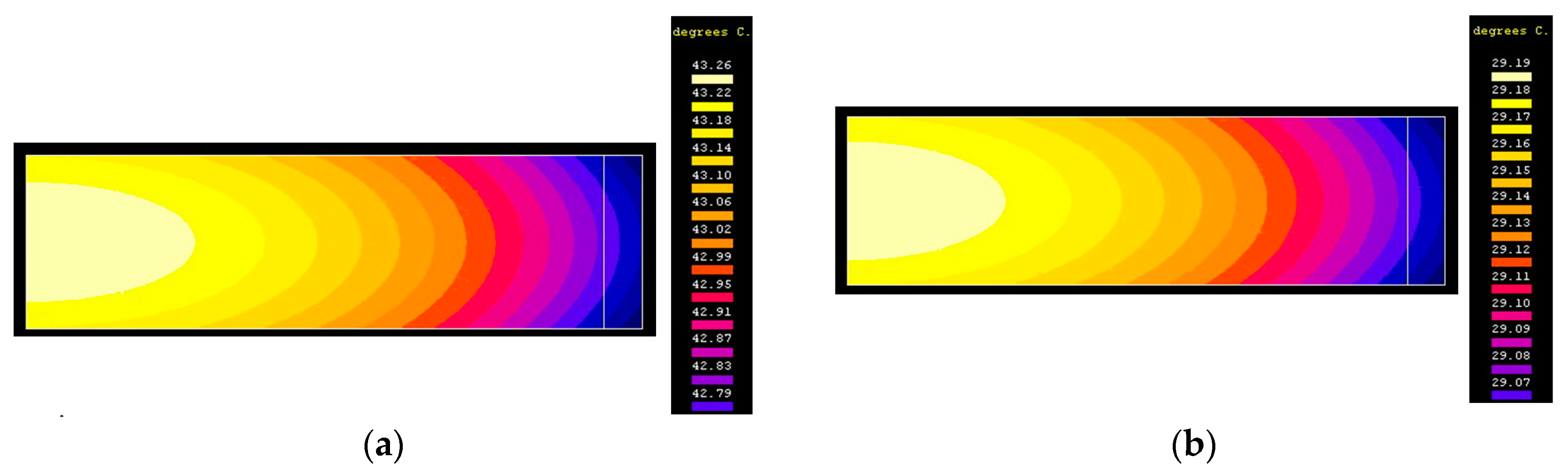
We will first present the results of the modeling in the situation of the independent varistor, which is not connected in parallel with any other. After instantaneous heating due to impulse application, varistor cooling is followed. This situation is important to analyze, especially when there is a risk of applying another impulse, at a short time (less than 10 min).
Figure 9a shows the temperature distribution in varistor
R at 60 s from impulse application.
Figure 9b presents the temperature distribution in varistor
R at 600 s from impulse application.
The maximum expected overheating to be reached during this process is (in °C):
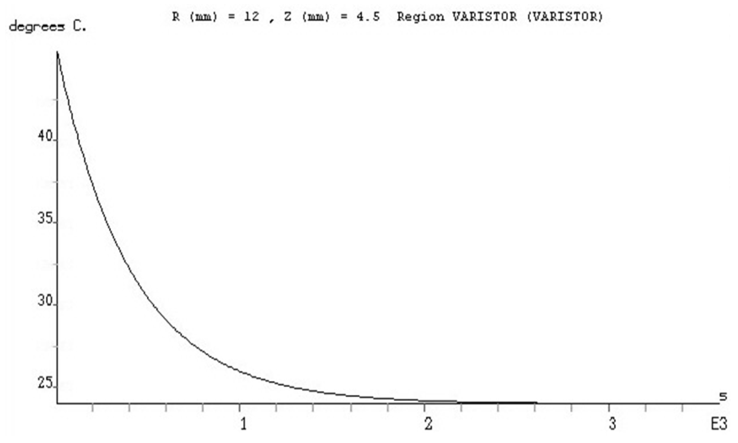
From where, the whole temperature is: θ = 24 + 23.89 = 47.89 °C. The value of the specific heat of the varistor at 20 °C was used as cv = 0.7534 (J/(g·°C)).
The over temperature measured immediately after the application of the impulse at a point located on the top of the varistor, at
R = 12 mm, is
t = 22.23 °C, which corresponds to a temperature
θ = 24 + 22.23 = 46.23 °C. In
Figure 10 we will present the time evolution of the temperature during the cooling process on one point having the coordinates:
R = 12 mm and
Z = 4.5 mm, as it results from the modeling performed on FLUX 2D.
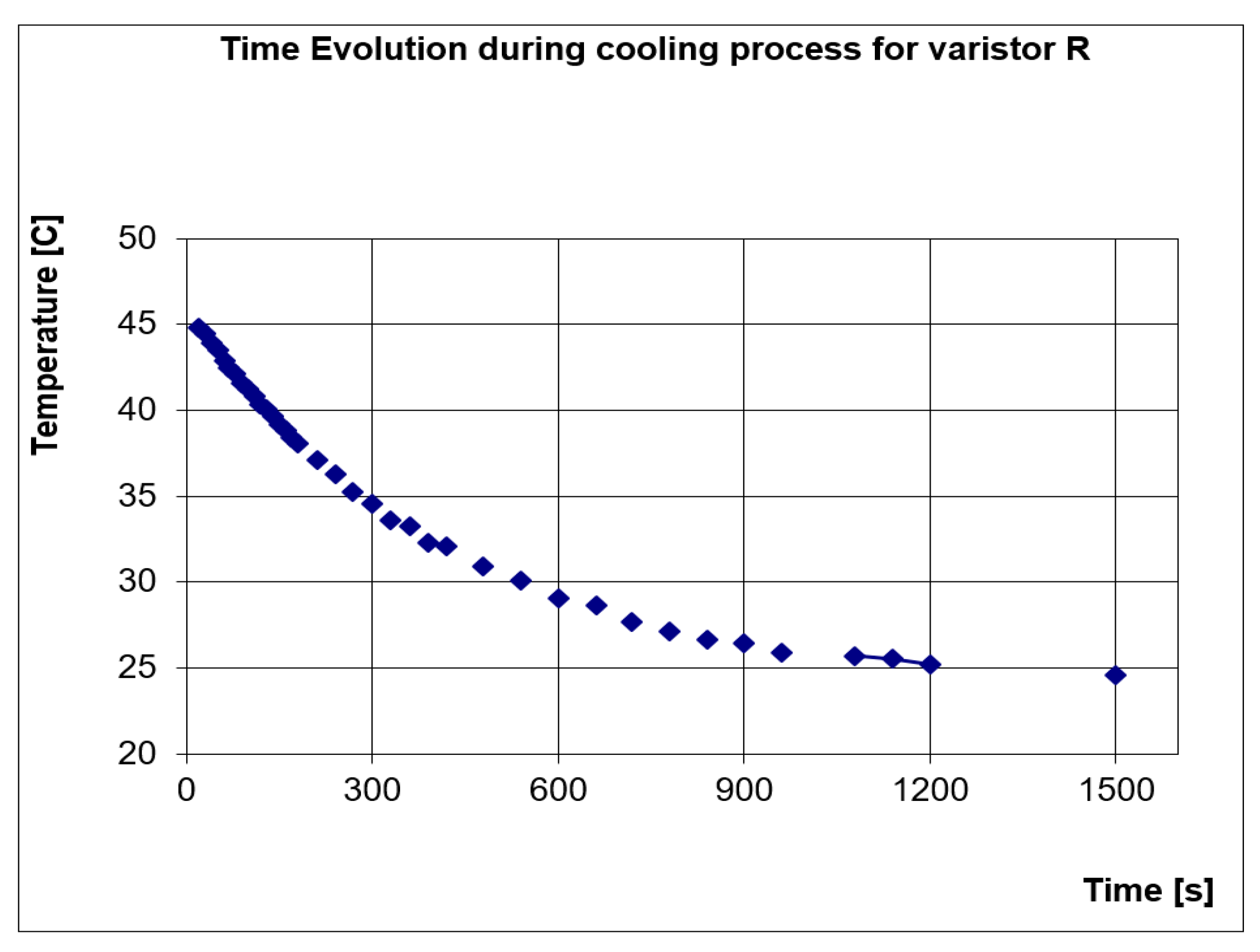
In
Figure 11 we present, for comparison, the temperature evolution over time, measured at the same coordinate point
R = 12,
Z = 4.5.
By comparing the two graphs we find that the two curves (the one resulting from the modeling and the experimentally determined) are quite close, so the experimental results confirm the numerical modeling.
There is still a major risk of overheating the varistor.
4.3. Analysis of the Impulse Regime for Two Varistors, in Parallel and Thermally Coupled
As in previous cases we will first present the results of the modeling in the situation of the independent varistor, which is not connected in parallel with any other.
Like in previous case, after an instantaneous heating due to impulse application, varistor cooling will be initiated, this issue is also important to analyze, especially when there is a risk of applying another impulse, at a short time distance (less than 10 min).
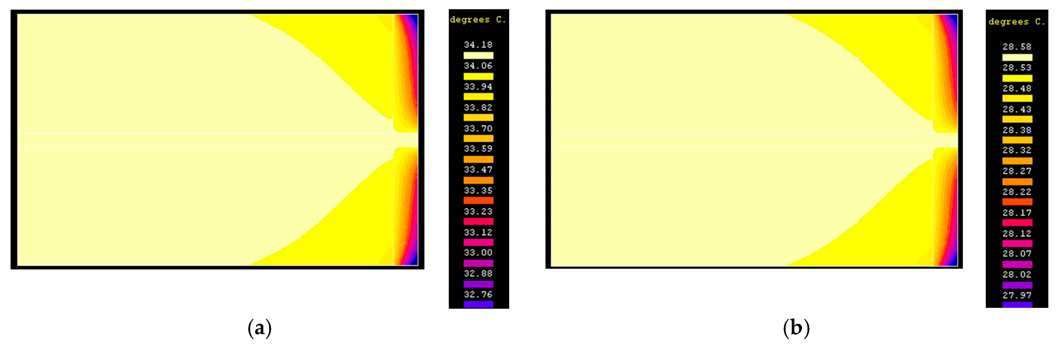
Figure 12a shows the temperature distribution inside the varistor assembly,
R +
S, in parallel and thermally coupled, at 60 s from impulse application.
Figure 12b shows the temperature distribution inside the varistor assembly,
R +
S, in parallel and thermally coupled, at 600 s from impulse application.
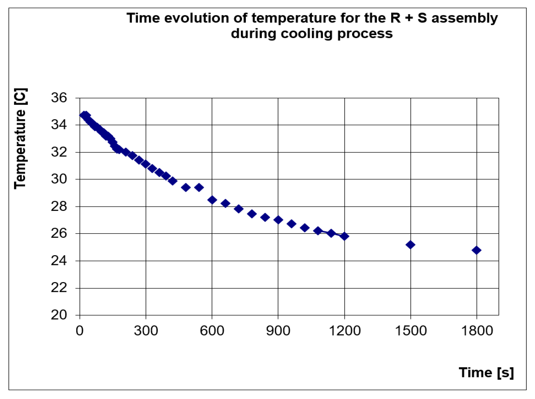
The cooling process of the varistors can be considered finished after approx. 1800−2000 s, but numerical modeling was performed over an interval of 3600 s. In this case, as in the previous situation, two temperature distributions obtained during cooling were presented at different time spans, when we have appreciable temperature differences between the various points of the assembly.
The over temperature, measured immediately after application of the impulse, on a point located on the upper surface of the varistor at R = 12 mm and Z = 4.5 mm, is t = 10.9 °C, which corresponds to a total temperature θ = 24 + 10.9 = 34.9 °C.
In
Figure 13 we present the evolution over time in the cooling process of the temperature at the coordinate point:
R = 12 mm and
Z = 4.5 mm, as it results from the modeling with FLUX 2D.
In
Figure 14 we present, for comparison, the temperature evolution in time, measured at the same coordinate point
R = 12,
Z = 4.5.
The maximum expected overheating to be reached during heating is, (in °C):
from where
θe = 24 + 11.23 = 35.23 °C.
The value of the specific heat of the varistor at 20 °C is cv = 0.7534 J/(g·°C) and the specific heat of the brass at 20 °C is cal = 0.383 J/(g·°C). We can notice that, even in this case, the experimental results are very close to the modeling results.
5. Discussion
The study of the thermal balance of a varistor must be done in all its operating regimes, because the danger of thermal runaway may occur at any time. Overheating of steady state thermal stability in permanent service is due to increased supply voltage or ambient temperature. The state of unstable thermal equilibrium is also reached during transitory (impulse) regime, when it is caused by the increase in the temperature of the varistor as a result of the heat storage in its mass.
The whole study was conducted with data acquired from some tests on low-voltage varistors. They were made by using an original manufacturing technology, developed by the authors at the "Génie Electrique"—Laplace Laboratory of the Paul Sabatier University in Toulouse, France. All measurements related to this paper were performed by using the equipment existing there.
The analysis of both situations (stationary and transitory) was started by performing a numerical simulation on an adequate thermal model. The use of a modular CAD package, in the modeling of thermal processes, is a necessary step in the design of any electrical equipment that is sensitively related to the evolution of its temperature or environment.
Because of the cylindrical symmetry of the parts used, it was not necessary to use a CAD package for three-dimensional modelling; all simulations were performed on a transversal section. The main elements of the FLUX 2D model are the mesh subdomains corresponding to the materials considered: varistor (colored in red); epoxy resin (colored in blue); brass (colored in yellow); The border areas are: brass border-air; the portion remaining in contact with the air on the top of the varistor; epoxy resin border air; lower varistor face; varistor-brass border; varistor boundary-epoxy resin; The model parameters of the considered materials and domains (both electrical and thermal) were carefully determined. The procedure and the results are very long to be explained in this paper and could be the object of another separate article, due to their highly dependence on temperature.
A simple solution which could be used for increasing the thermal stability of varistors integrated in surge arresters consists in a parallel connection of them. In this case, if they are placed separately and their electrical characteristics are very different, there is a risk that only the varistor which has a lower clamping voltage to support the whole pulse. By consequence, the parallel connected varistors must be forced to act as simultaneously as possible, and equally take over the energy resulting from the application of the voltage impulse.
This technical solution is not so useful in permanent regime, mostly because each varistor losses a lateral heat dissipation surface. It is not so dangerous, and it could be compensated by increasing the lateral surface of the junction additional mass.
The material used by the authors for the junction additional mass located between the varistors is brass, due to its main properties:
cheap material;
easy to process;
good thermal conductor;
specific heat sufficiently high;
reduced electrical resistivity;
can be welded with tin on the varistor surface;
the material parameters are well-defined and well-known;
used in the construction of electrodes from surge protection equipment.
The main potential applications of these research will consist in construction of new varistor devices with increased thermal stability (which is also the most important benefit obtained from researches like this one). The main application domain is the low voltage surge arrester market, mostly when thinking on the mandatory requirements which could be introduced for low voltage protection devices inside all domestic installations.
We will focus on two new technical solutions issued from this research:
A “sandwich” varistor device, made of two similar varistors connected in parallel and thermally coupled throughout a metal mass, like in this research;
Another variant of the sandwich type varistor group, with a bigger additional mass, in order to evacuate more heat from the varistors’ cores.
Both solutions could be applied, with correct dimensions, to all voltage levels.
6. Conclusions
Parallel connection of varistors may be a technical solution worth taking into account only under certain conditions. In permanent service, the parallel connection of the varistors does not bring any improvement in their operation. Moreover, in the case of thermal coupling between varistors, loss of a face as a heat dissipation surface, the varistor operates at a higher temperature than if it operated independently.
In impulse service mode, that impulse energy is allocated to the two varistors, depending on the electrical characteristics of each one. From a theoretical and experimental point of view, if the two varistors have close electrical characteristics, the over temperature reaches almost half the value that would have been in the case of a single varistor. If there is no thermal coupling between the two varistors, the dissipation of the accumulated heat will occur faster. As a result, the technical solution of the operation of parallel varistors with thermal coupling significantly increases the thermal stability of the equipment in which they are embedded, when the varistors have almost identical performance.
The thermal coupling between varistors becomes useful only when the electrical characteristics of the two varistors are different (first there are differences of up to 5% between the UN threshold voltages of the two). Even if the loss of a radiant surface makes cooling difficult, the thermal coupling leads to the equalization of the temperatures in the two varistors and thus determines the uniform distribution of energy in the mass of the two varistors. Otherwise, the varistor with the lowest threshold voltage will take up most of the impulse energy, which will lead to unwarranted heating, and there is even the risk of thermal runaway after the impulse passes, the varistor remaining polarized at the rated voltage of the grid, but at a temperature that causes a sensitively higher current than the normal current flow. Thermal instability can also be achieved by applying successive pulses at intervals of less than 10 min, occurring when the varistor receiving the impulse is already heated at a high temperature.


