Abstract
The modular multilevel converter (MMC) has been prominently used in medium- and high-power applications. This paper presents the control of output and circulating current of MMC using sliding mode control (SMC). The design of the proposed controller and the relation between control parameters and validity condition are based on the system dynamics. The proposed designed controller enables the system to track its reference values. The controller is designed to control both output current and circulating current along with suppression of second harmonics contents in circulating current. Furthermore, the capacitor voltage and energy of the converter are also regulated. The control of output current is carried out in -axis as well as in with first-order switching law. However, a second-order switching law-based super twisting algorithm is used for controlling circulating current and suppression of its second harmonics contents. The stability of the controlled system is numerically calculated and verified by Lyapunov stability conditions. Moreover, the simulation results of the proposed controller are critically compared with the conventional proportional resonant (PR) controller to verify the effectiveness of the proposed control strategy. The proposed controller attains faster dynamic response and minimizes steady-state error comparatively. The simulation of the MMC model is carried out in MATLAB/Simulink.
1. Introduction
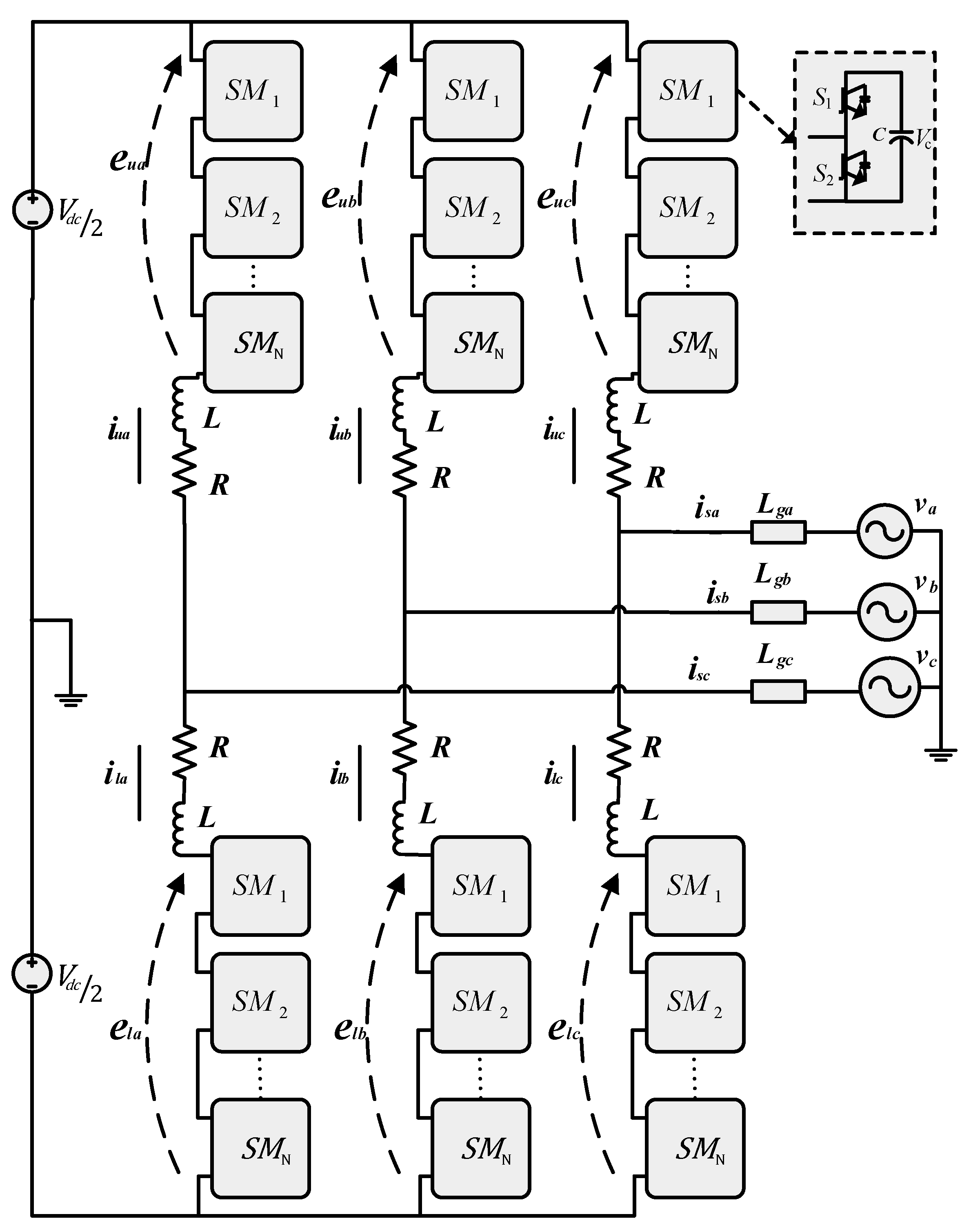
The modular multilevel converter has been widely used in medium and high-voltage applications [1,2], integration of renewable energy [3,4], medium-voltage drives [5,6], and battery energy management system [7,8] due to its versatile and promising features i.e., modularity, redundancy, excellent harmonic performances, and transformerless configuration [1,9,10,11]. The structure of modular multilevel converter (MMC) is composed of different modules connected in different configuration i.e., half-bridge and full-bridge, as depicted in Figure 1.

Figure 1.
3 Phase circuit diagram of modular multilevel converter (MMC).
The control of MMC is categorized into internal current control and output current control. Output current control is used to control the active and reactive power of converters [9,12]. Along with the control of output power, the internal dynamic of MMC i.e., circulating current and submodule capacitor voltage, is also in focus. In order to achieve multiple objectives i.e., energy balancing, circulating current control, and output current control, various control schemes have been introduced in the literature.
The control scheme introduced by Hagiwara and Akagi [13] is mostly adopted in the literature. The circulating current control is used to suppress the harmonic contents produced due to capacitor ripples. The magnitude of circulating current has a high impact on the arm current. It increases the root mean square (RMS) value of arm current, which will increase power losses and second-order harmonics will result in further generation of other higher-order harmonics that will increase power loss and current stresses on switching devices [14,15]. However, no impact of circulating current is seen on the alternating current (AC) network.
A different current control method is proposed, such as control using proportional-integral controller [16,17]; the output current is controlled in with grid frequency while the control of circulating current is carried out in double frequency frame. But the controller fails to completely suppress harmonics in circulating current due to limited gain at harmonic frequencies. This will result in the insufficient performance of MMC in a steady state. PR controller is also proposed in [18,19] to control the circulating current. However, the design and tuning of multi-resonant control is difficult and complicated. Moreover, any small deviation in frequency will lead to a larger deviation of the control variable from its reference. In [20,21,22,23], the authors proposed a harmonic repetitive controller and plug-in repetitive controller for suppression of second harmonic in circulating current, but achieving a stable operation and excellent control performance may be a trivial task. Furthermore, these controllers are tuned at a specific frequency, and a small variation in frequency can lead to the failure of the controller. A combination of spatial comb and the spatial repetitive controller is proposed in [24] for suppression of second harmonic current and controller of output current, but the author has not discussed the balancing of capacitor voltage and energy of converter. A sliding mode controller is proposed in [25] to control the current of the converter, but the author does not consider the store energy and energy difference between arms. Moreover, the circulating current is controlled in a double-frequency frame. Interconversion of different frames will cause a computation burden for a large system. In [26], sliding mode control is proposed only for controlling the output current, although the circulating current and energy balance of the converter is not considered. Moreover, the circulating current is controlled in the dq-axis frame. Hence, interconversion of the different frames will increase the computational burden. The arm inductor also has a prominent effect on the circulating current studied in [27], but the large value of inductor will result in bulkiness of the converter. A backstepping controller is introduced in [28] to eradicate the harmonic content of circulating current. Although the amplitude of second harmonic current is reduced, it is not eliminated completely. A feedback linearization [29], model predictive approach [30,31,32], and langrage optimization-based control [33] was proposed to control parameters of MMC but the computational complexity, a well-developed mathematical model, and variable frequency operation limit the effectiveness of these strategies.
In order to cope with the problem and complexities of different control strategies, SMC [34] is proposed for controlling output current, circulating current, capacitor voltage, and energy balance of MMC. The indirect SMC control can be easily adapted for power converters. The remarkable characteristic of SMC is its easy and simple implementation and tuning. Moreover, the response of a closed-loop system becomes insensitive to some uncertainties due to the use of SMC. This principle will cope with the intrinsic model variations. Furthermore, the implementation of circulating current control in ABC frame will reduce the computation burden of different transformation () needed during desigthe n of control schemes. The two terms of control law i.e., equivalent term and attraction term, will combinedly move the system trajectory to the sliding surface and keep it steered on it. The condition of attraction is satisfied by choosing a proper derivative. A first-order SMC is designed for output current control in . However, a second-order SMC based on the super-twisting algorithm is designed to suppress the second-order harmonic current and steer the value of circulating current on the DC reference.
2. Modeling of MMC
The equivalent single-phase circuit of MMC is depicted in Figure 2. The different currents flowing in arms of MMC are defined as [35]
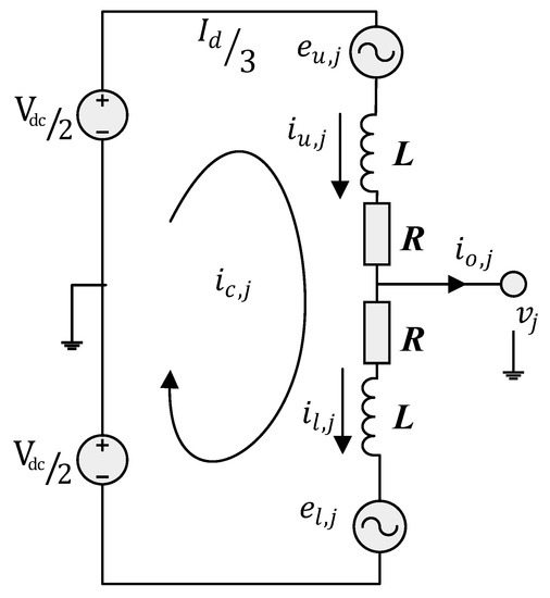
Figure 2.
Phase equivalent circuit of MMC.
By applying Kirchhoff’s voltage law on the upper and lower arm of the circuit in Figure 2, we get the following voltage equations
Adding and subtracting Equations (5) and (6), along with the substitution of Equations (3) and (4), will result in a new set of equations given as
Equations (7) and (8) characterize the dynamics of MMC. By analyzing Equation (7), it is concluded that as is AC bus voltage, only can be manipulated to control outputhe t current . Similarly, Equation (8) is used to control the circulating current dynamics of MMC. Likewise, in Equation (8), can be controlled by manipulation of the internal voltage . Moreover, the internal dynamics of the SM capacitor also has a great effect on the circulating current. It is represented in terms of arm voltages and arm currents as
, means the capacitor is inserted while , means the capacitor is bypassed in respective arms. Equations (8)–(10) combinedly represent the internal dynamic of MMC.
Equations (1) and (2) are substituted in Equations (9) and (10) to represent capacitor dynamics in terms of output current, circulating current, and insertion indices (, ).
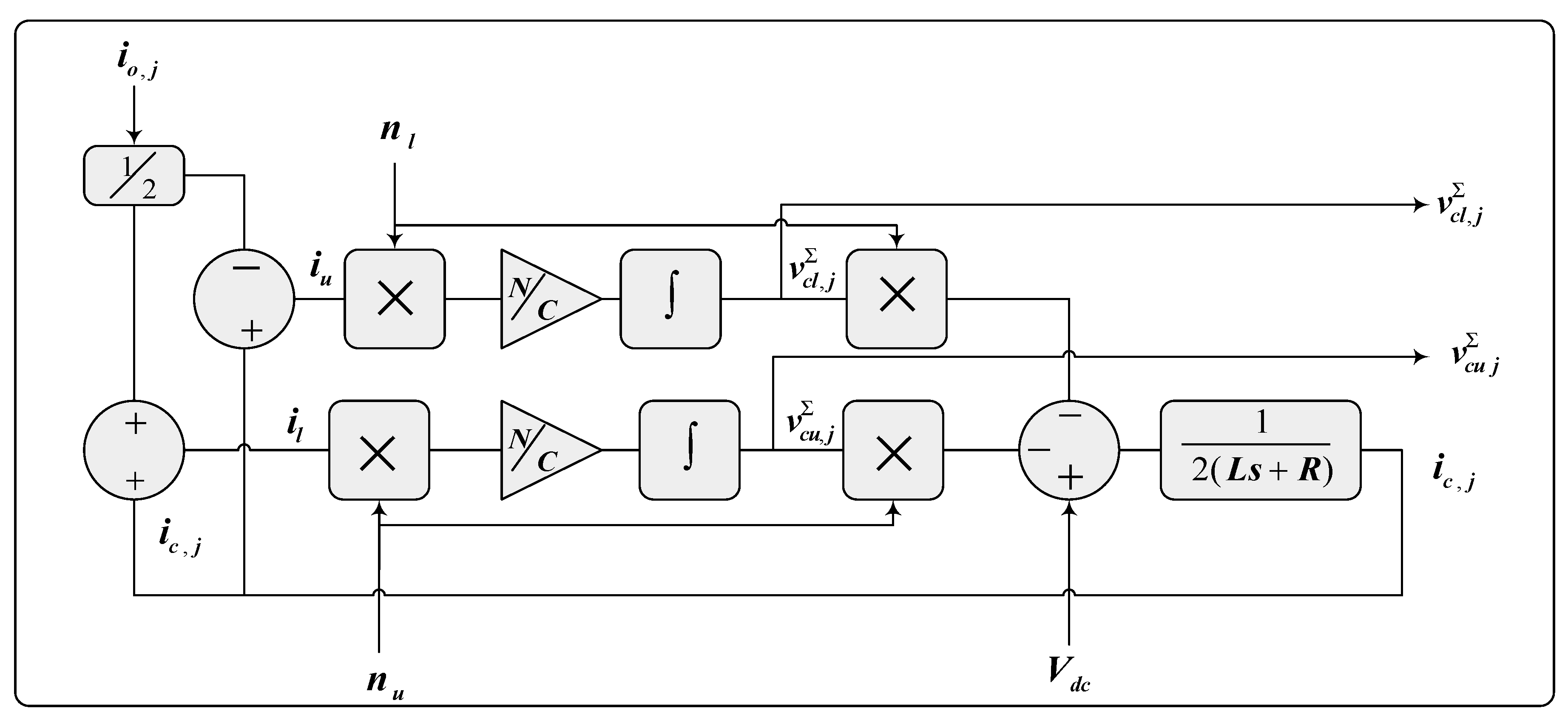
While and , and are the controlled inputs to the plant. The internal dynamic of MMC is controlled through the convergence of to a DC component . In control of MMC, and are available for manipulation. Also, and are forced to converge to for controlling the internal dynamics of MMC. Equations (1)–(12) are modeled in MATLAB/Simulink as depicted in Figure 3.
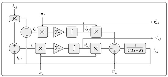
Figure 3.
Simulink model.
3. Control Structure of MMC
3.1. SMC Design Overview
SMC has the remarkable properties of easy tuning, robustness, accuracy, and easy implementation. These features allow for the use of SMC in various domains for controlling nonlinear processes. Hence, SMC is used in control of different applications such as electrical drives [36,37,38], power converter converters [39], microgrid control [40,41], wind energy control [42], and many more.
The SMC system is designed to steer the states of a system onto a specific surface in state space, called the sliding surface. The two conditions, invariance and attractivity, made the trajectory steer on the sliding surface. The conditions are given as
The condition given in Equation (13) defines the control law for a given system. The control law is composed of both invariance and attractive condition. The mathematical expression for control law is given as
represent control input to the plant. , represents invariance and attractive terms respectively. The two terms in control law have distinct features.
- The first term is equivalent control, which keeps the system trajectory on a sliding surface.
- The second term is used for attractivity; it brings the system from outside to the sliding surface. Usually, it determines system dynamics from initial point to sliding surface.
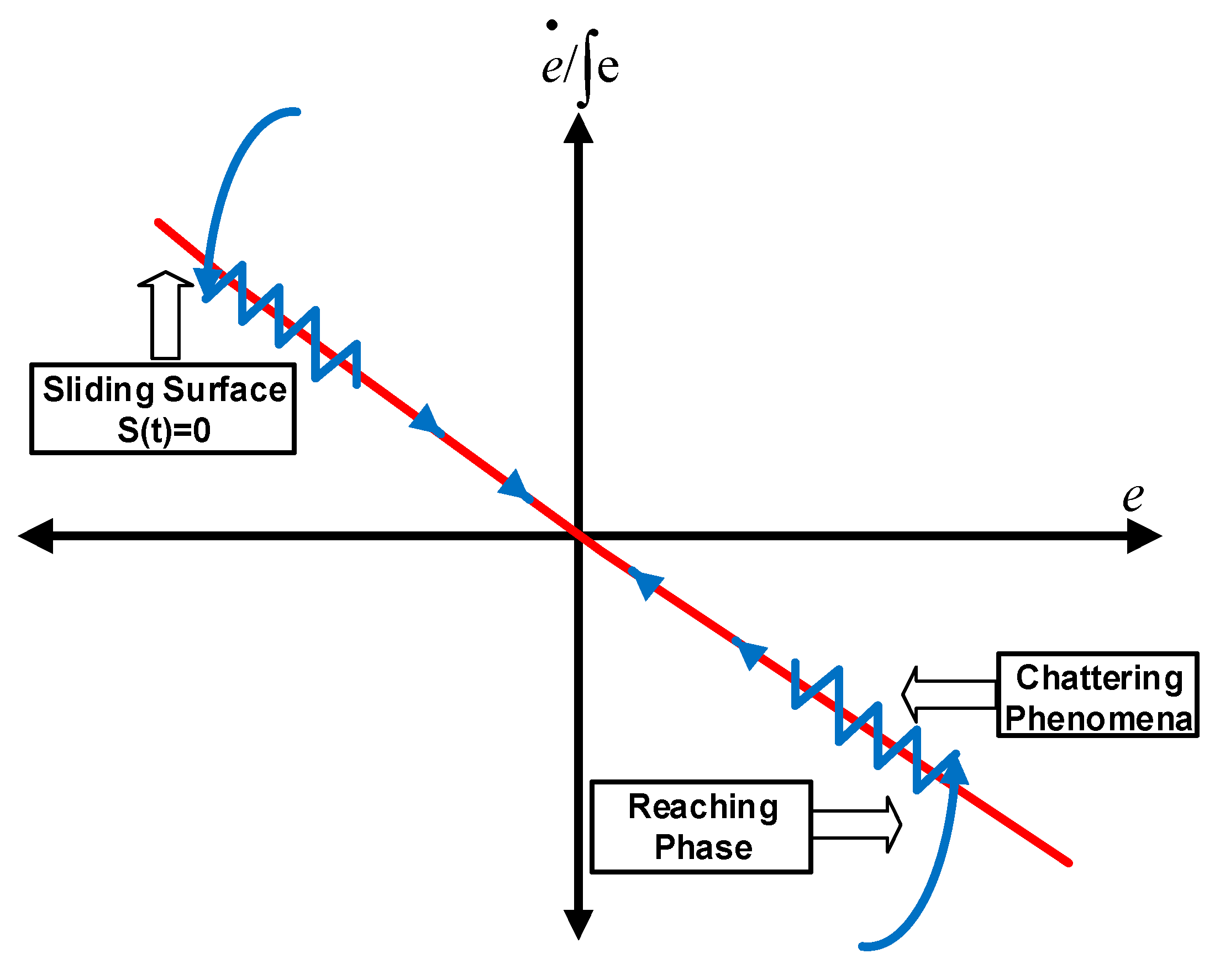
Both the above conditions are graphically illustrated in Figure 4.
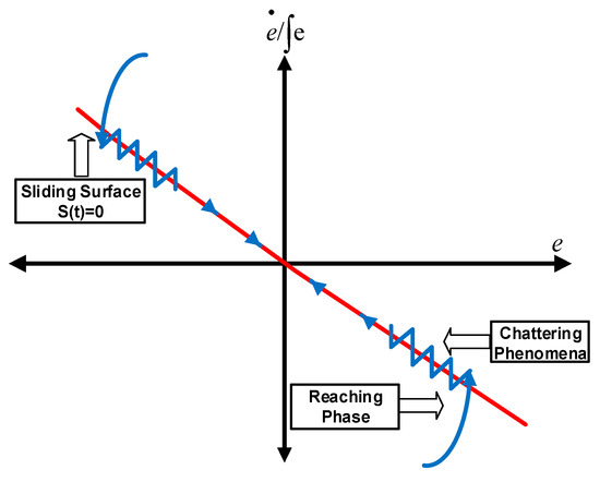
Figure 4.
Sliding surface.
Consider a nonlinear system described as in [43] for designing of control law
where is the system state vector and and are a nonlinear function of the system state vector and input vector . The switching function for a system is defined as
where are the coefficients of the sliding surface. The derivative of the sliding surface is given as
Substitute the value of in Equation (17)
by assuming the reaching law
while and are positive real numbers. Combining Equations (15)–(19) we get control law as
Equation (20) gives the control input to the plant. By choosing a proper value for and , the system output parameters will follow the desired performance.
SMC is very effective in the control domain, but an undesirable chattering problem is associated with it, as depicted in Figure 4. This should be eliminated as it gives rise to oscillations and appears in the output. Different techniques are used to solves chattering issues. In our control scheme, we use the saturation function for output current loop as described in [40,41], while the super twisting algorithm is used for control of circulating current to cope with this issue effectively. The second-order algorithm makes the law continuous; hence, it handles the chattering issue in a very efficient way.
3.2. Output Current Control
The dynamics of the output current are shown in Equation (7). As it is clear from the equation that is available for manipulation to control the output current, Equation (7) can be also be presented in the below form
Equation (21) is transformed from to using Park’s transformation () [16].
For balanced three-phase system, Equation (21) can be represented in as
Equation (23) is used to formulate the control law. The control law is formulated by considering both invariance and attraction condition as
The first terms in Equations (24) and (25) represent the equivalent voltage vector. The equivalent voltage vector is active during steady-state, and it will steer the system trajectory onto the sliding manifold, while later terms in Equations (24) and (25) represent attractive voltage that is active in the transient state. The attractive term forces the system trajectory to the sliding surface. The error for both d-axis and q-axis current is defined as
The relative degree of the system is . Hence, the sliding surfaces selected for and are as follows
The and terms that are calculated from Equations (27) and (28) given as
By simplification of Equations (29) and (30), we can get an equation for the invariance condition of the design controller.
From Equations (26) and (27), and replace the value in Equations (29) and (30), and solve for the value and given as
The switching functions and used in control law are given as
The and terms force the state trajectory to approach the sliding surface. The rise time will reduce with a larger value of while a small value of will minimize the oscillation. The fully controlled law is given as
while
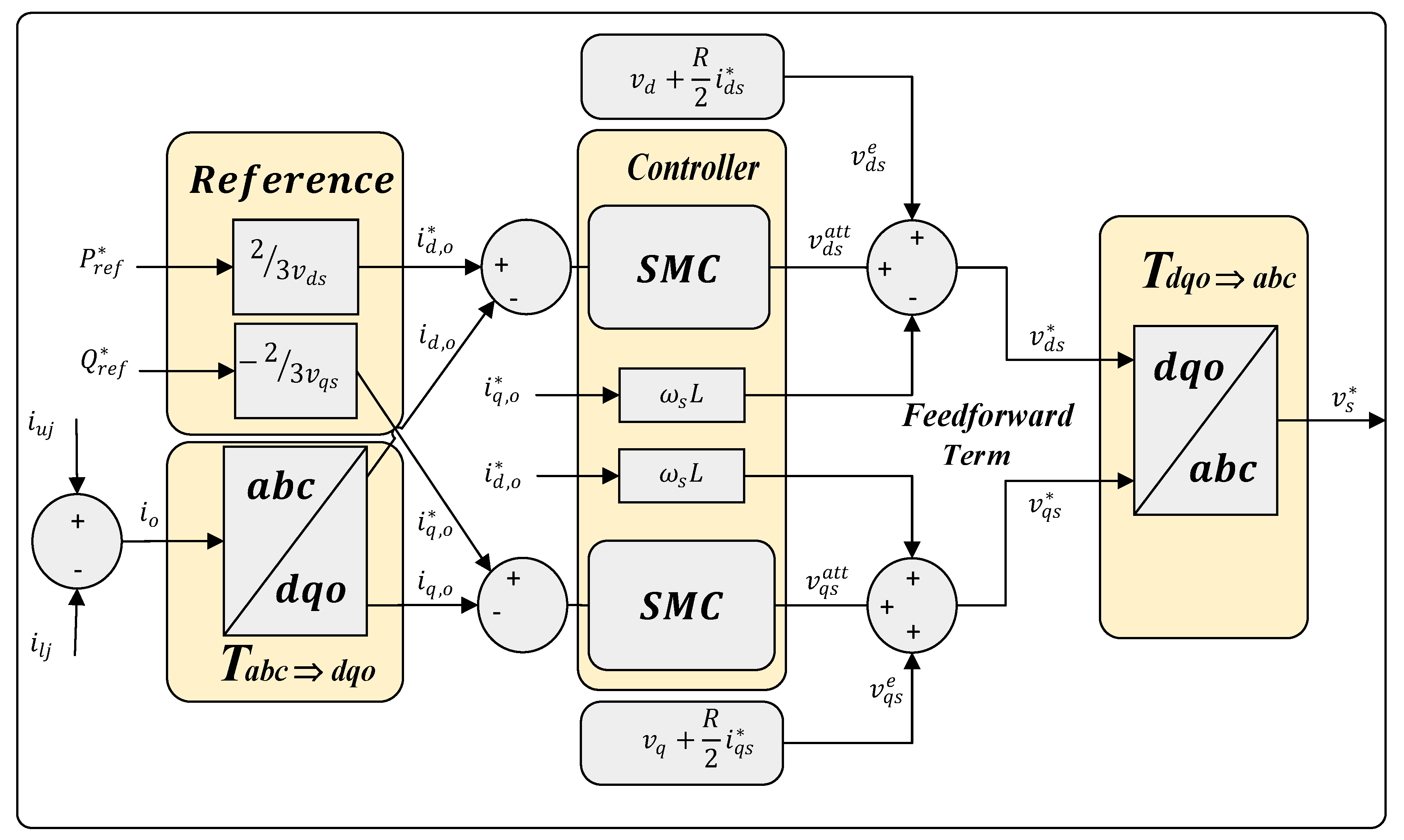
The implemented control structure for output current control is depicted in Figure 5.

Figure 5.
Output current control structure.
Theorem 1.
The proposed designed control scheme based on SMC is asymptotically stable and ensures boundedness of tracking error of output current if the reference dq-axis voltageis chosen as in Equation (37).
Proof of Theorem 1.
The stability of the system can be checked using Lyapunov stability analysis [43].
A Lyapunov function is defined as
In order to ensure the stability of Equations (33) and (34), the following two conditions need to be satisfied
In order to check the first condition of Lyapunov stability, the derivative of Lyapunov is given as
The value of is substituted from Equations (29) and (30)
Similarly, from Equations (33) and (34)
The value of is substituted into Equation (43). The equation is modified as
Substituting the value of Equation s(27) and (28) and Equations (35) and (36)
This equation for q-axis current returns a negative value regardless of the sign of sliding surface and that ensures the stability of the system. However, for d-axis, Equation (44) shows that for any value of switching function, the derivative of the Lyapunov equation is negative. Similarly, the second condition of stability is also fulfilled. □
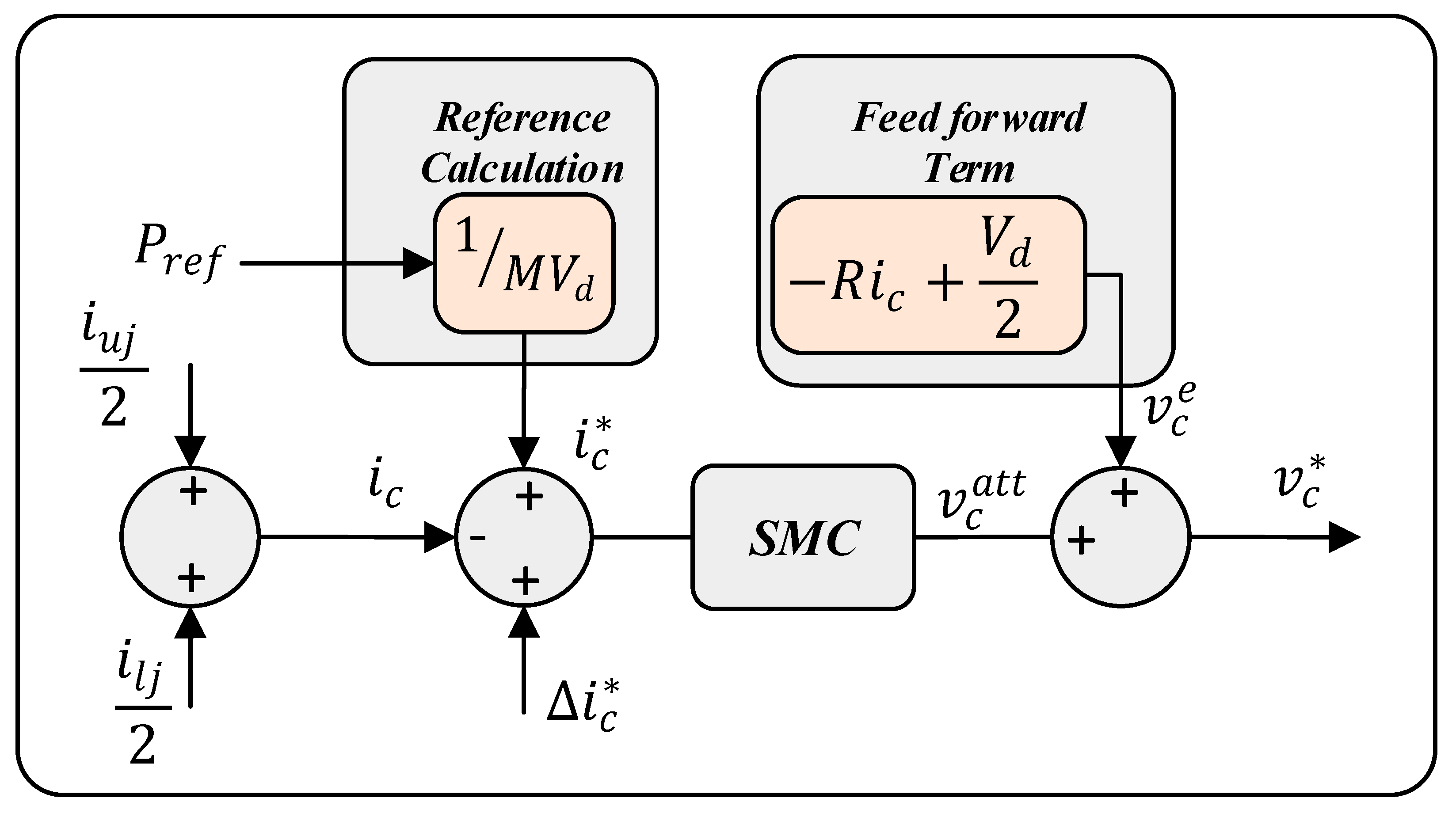
3.3. Circulating Current Control
The circulating current is generated due to the inner voltage imbalances between the arms. It flows in each phase leg of the converter. Circulating current is in the form of a negative sequence current with double grid frequency [16]. It does not affect the output current or voltage, except it increases the losses of converter. The circulating current has two parts is given as
The value of is forced to follow DC current (), which will result in the suppression of second harmonic current. The switching law for the circulating current control is composed of equivalent voltage and attractive voltage.
Similarly, the switching function for circulating current control is given as
By taking the derivative of Equation (49) and substituting the value of from Equation (8), we get
By solving Equation (50) for equivalent voltage ‘’,
Substituting Equationa (51) and (49) in Equation (48), we get
In order to converge switching function to zero, the super-twisting algorithm is used for circulating current. Due to its continuous nature and integral term, it will compensate for the high-frequency disturbances i.e., second harmonic current. It will retain the continuity of function along with attenuation of disturbance. The super-twisting control algorithm is given as
where . The larger value of will result in a good performance of the closed-loop system. This second-order controller will reduce the oscillatory contents of circulating current and will track the DC reference effectively. Equations (51) and (53) combinedly givesthe control law for circulating current control. The overall equation is given as
will provide a controlled input to the plant. The reference value of circulating () current is one-third of DC current. Along with the DC component, an increment derived from the energy equation is added to the reference to keep the converter’s energy balanced. The energy balancing technique used in [44] is adopted in this paper. The time derivative of energy sum and energy difference is given as
and . In order to enhance the performance of circulating current controller, the mean value of and is made equal to by converging to and to zero. Equations (55) and (56) are integrated to get and as in [35]. Hence, the increment term is obtained
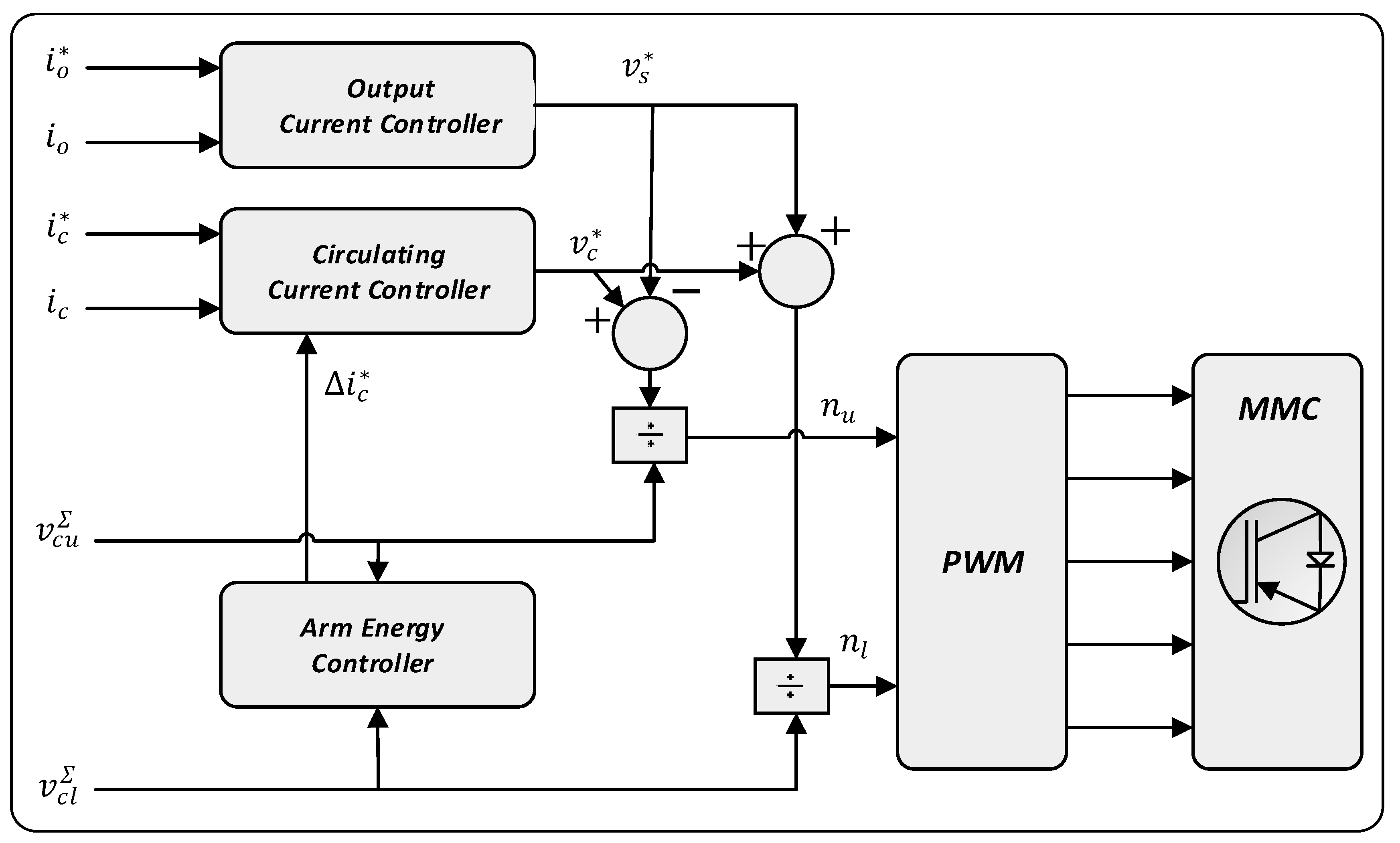
represents low pass filter, and and are positive constants. The control structure for circulating current control is depicted in Figure 6. However, the overall control scheme implemented for control of MMC is depicted in Figure 7.
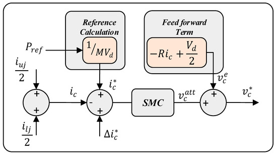
Figure 6.
Current control structure.
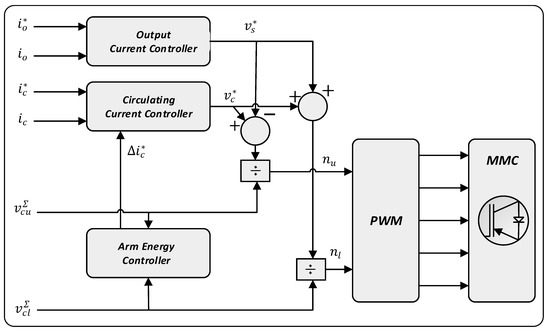
Figure 7.
Structure of MMC.
Theorem 2.
The proposed designed SMC-based control scheme for circulating current is asymptotically stable and ensures boundedness of tracking error if the reference internal voltageis chosen as in Equation (54).
Proof of Theorem 2.
Like the output current controller, the stability of the circulating current controller is also ensured. From Equation (42), in the case of the circulating current controller, the value of the switching function is substituted from Equation (49)
is calculated as
The value of is substituted into Equation (59), and simplifying the equation,
Finally, the value of is substituted with Equation (53)
Hence, if
In the case of the circulating current controller, Equation (62) should be satisfied for the stability of the system. However, the second condition of Lyapunov is satisfied.
4. Results and Discussion
A three-phase model of MMC is simulated in MATLAB/Simulink to analyze the performance of the design control scheme. The value of different parameters is presented in Appendix B. The simulation was carried out for 1 s, but to show the transient response, the time axis is scaled to 0.3 s. Moreover, the scale of the y-axis is kept the same for easy visual comparison.
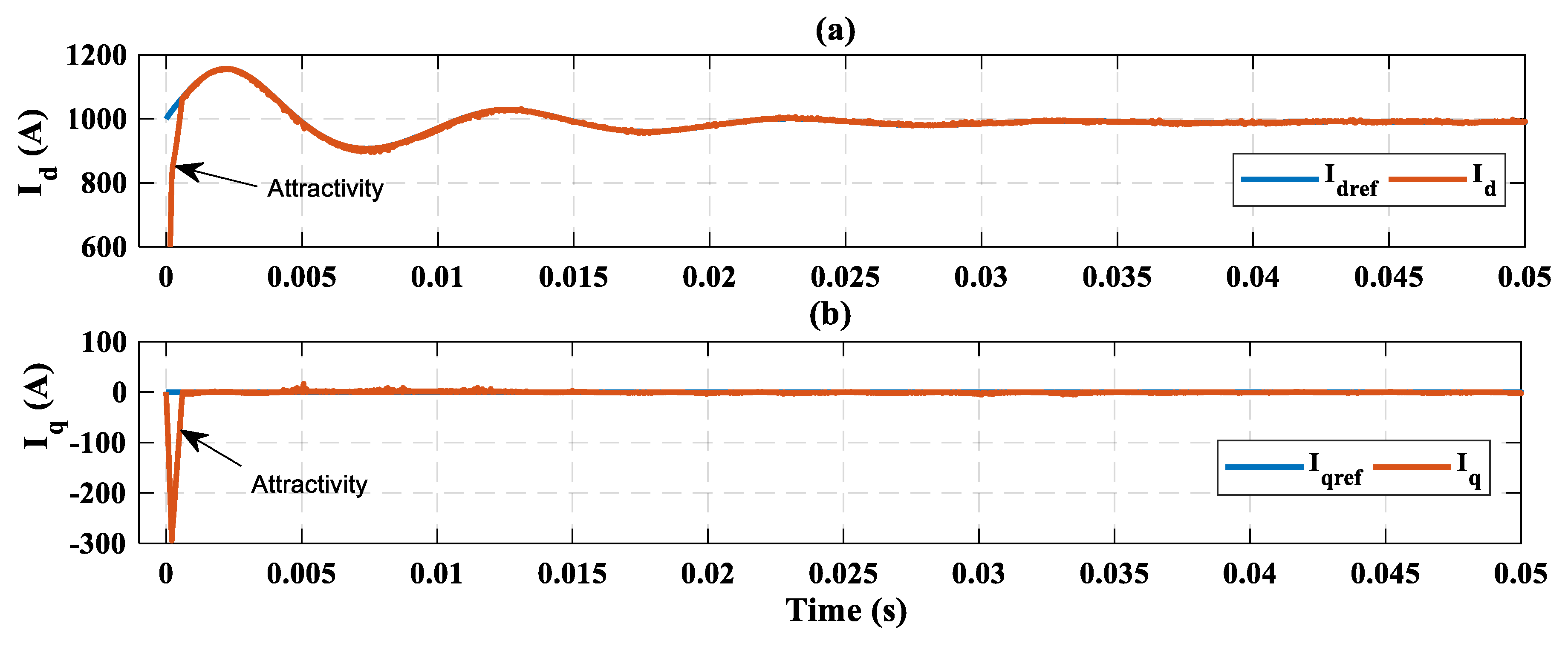
The output current of MMC is transformed and controlled in - axis. However, for the sake of comparison with the PR controller, the output current is also controlled in a stationary frame . The reference value of output current is generated from the desired active power and reactive power. The measured values of output current () track their respective references perfectly as depicted in Figure 8a,b. The d-axis and q-axis currents are attracted to the reference values and perfectly follow it. The designed controlled attractive term and equivalent term contribute well in achieving control goals. The system reaches steady-state at . The controlled value of these currents ensures that MMC is delivering the desired active and reactive power to the grid. The response of proposed SMC is fast and efficient as the controller works well in dynamic as well as in steady-state.
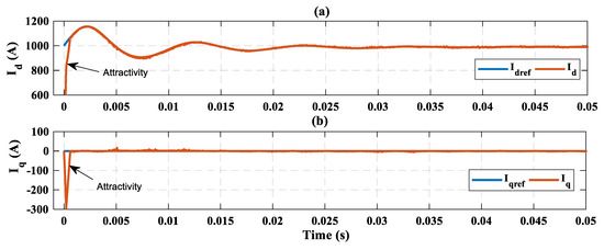
Figure 8.
Output current; (a) d-axis current; (b) q-axis current.
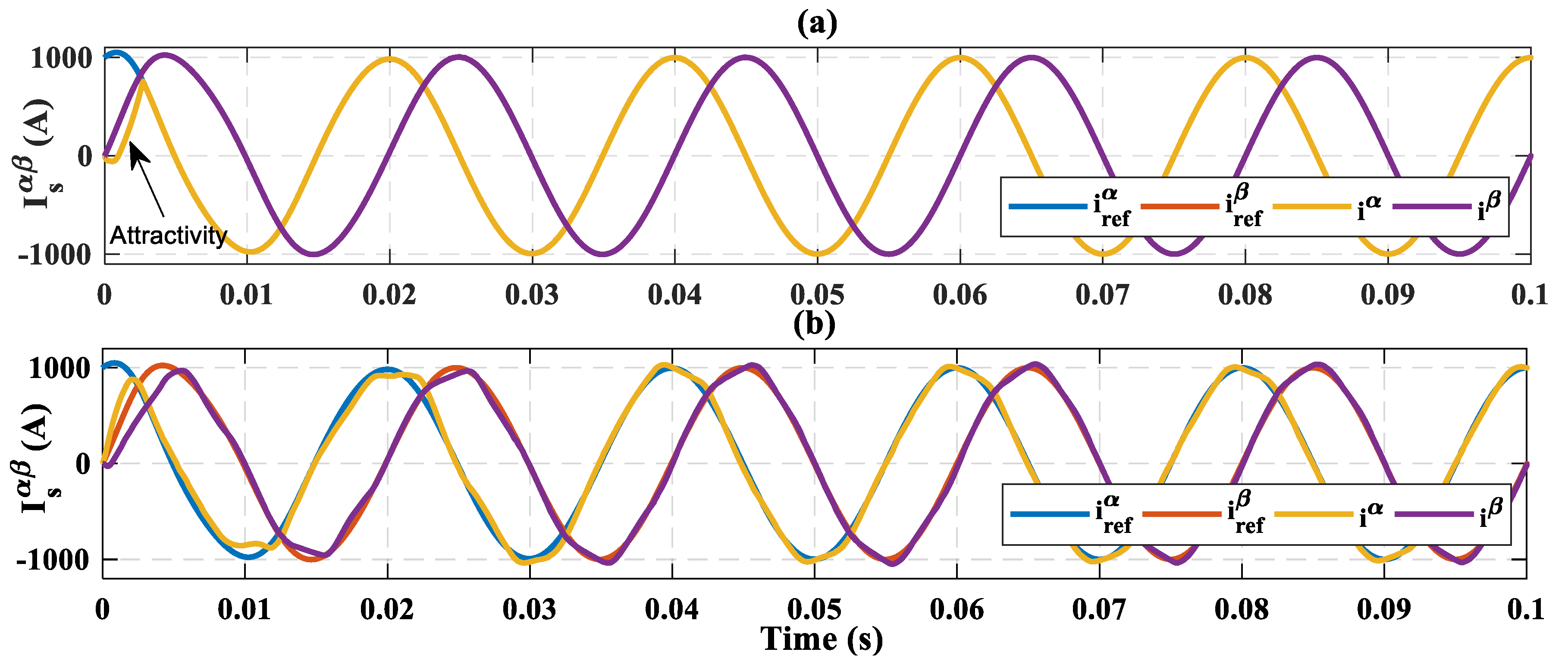
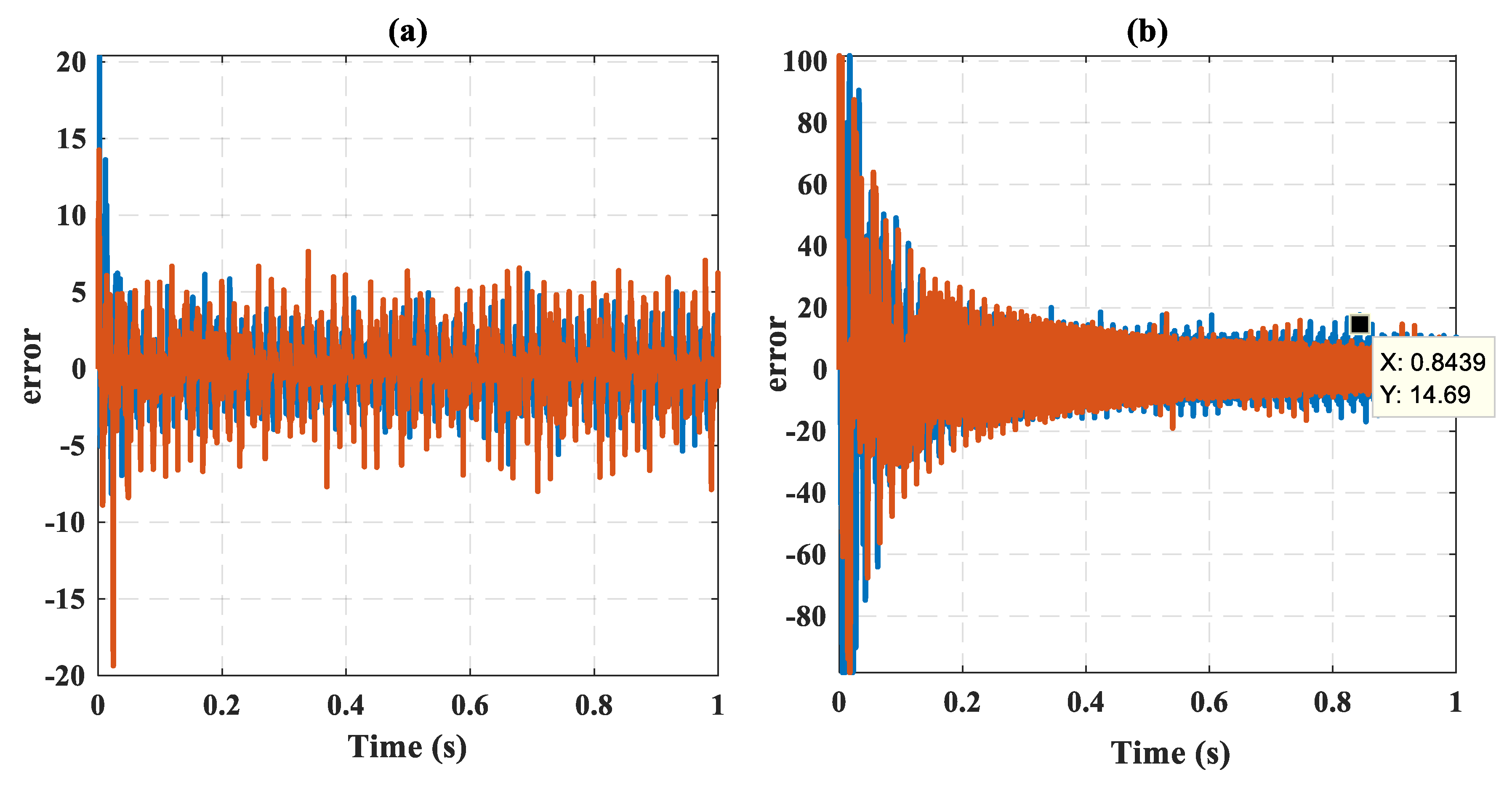
Figure 9 shows the control of output current in the stationary reference frame. The results of the proposed controller are compared with PR. The control law developed in the case of a stationary reference frame is given in Appendix A. Figure 9a shows output current controlled through SMC while the control of output current through PR is depicted in Figure 9b. The comparison of both controllers shows that the SMC is capable of reaching the respective reference value quickly, which shows the fast response of the proposed controller and perfect tracking of the desired value with almost zero steady-state error. As an initial condition for the sliding surface is zero, -axis current catches its reference values right from the start and the attractive term of controller helps -axis current to reach its respective reference. After reaching the reference, the equivalent term perfectly keeps the measured value on the track to minimize steady-state error, while in the case of the PR controller, the transient response of the controller is slow. It takes too much time to track the reference value. However, the response gets better in steady-state; but the steady-state error still exists. The error of both controllers is represented in Figure 10, and provides a clear comparison of both controllers. Figure 10a shows that SMC has an error of 5 A both in transient and steady-state, but the PR has a peak of almost 100 A in transient while 20 A in steady-state. This shows the crystal-clear effectiveness of the proposed controller.
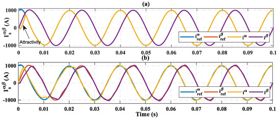
Figure 9.
Output current in αβ-axis and its references; (a) control using sliding mode control (SMC); (b) control using proportional resonant (PR).

Figure 10.
Error signal of output current; (a) SMC; (b) PR.
Figure 11 shows the reference and measured values of circulating current (). The reference of is set according to value i.e., 250 A. The convergence of ensures that the second harmonic current flowing in each leg of the converter is suppressed and only the DC component of the current is flowing in each leg. Consequently, it will result in the reduction of converter losses and reduces current stresses on the switches. Figure 10a,c shows the dynamic response of circulating current using SMC and PR controller, respectively. The response of SMC is fast and efficient as it reaches a steady-state in 0.05 s while PR takes almost 0.15 s to reach a steady state. This shows the response of SMC is three times faster than PR in case of circulating current control. The responses in steady-state are given in Figure 11b,d for SMC and PR controllers, respectively. The effectivity of SMC is persistent in steady-state as well. The current is converged perfectly at reference value in the case of SMC while the response of PR is subjected to large amplitude oscillation and different current is flowing in different legs of MMC. Notably, phase C has a large deviation from the desired value. The difference between the measured value and the reference value is almost 20 A. Besides this difference, the second harmonic contents of circulating current still exist. The PR controller fails to fully suppress the second harmonic current. This will lead to more converter losses and current stress in devices for the same size and rating of converter.
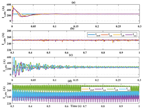
Figure 11.
Current with references (a,b) control with SMC; (c,d) control with PR.
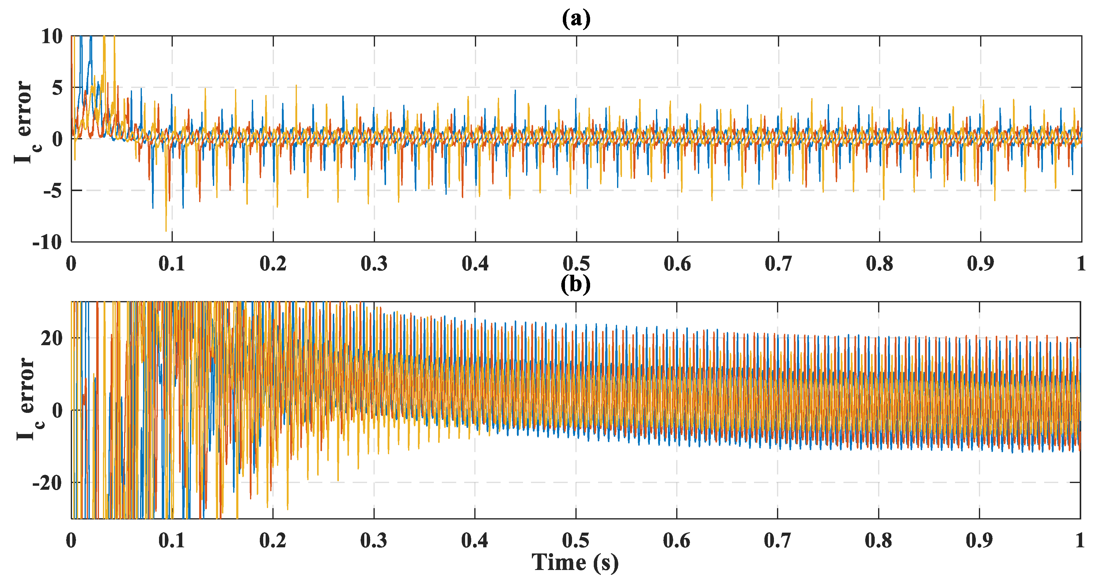
Figure 12a,b shows the error of circulating current. As it is clear from Figure 11, the error has an amplitude of about 200 A up to t = 0.05 s while after the dynamic response, still there is a large steady-state error that exists in the case of the PR controller. However, the SMC has a good contribution toward achieving the control goal. The error in the case of SMC has an amplitude of maximum of 5 A in steady-state.
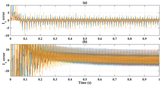
Figure 12.
Circulating current error; (a) SMC; (b) PR.
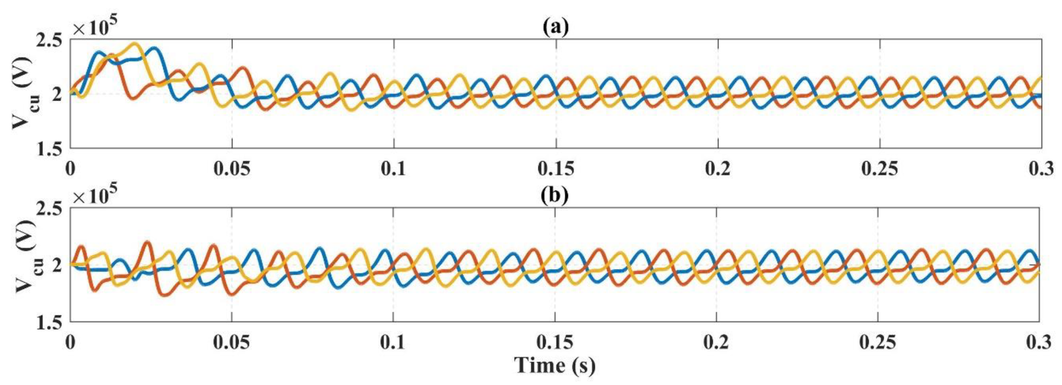
The response of the upper arm capacitor voltage is depicted in Figure 13. This response of the lower arm capacitor voltage is not shown as both the upper arm and lower arm have almost the same response. Figure 13a shows the capacitor voltage response in the case of SMC while Figure 13b shows the capacitor voltage in the case of the PR controller. As both controllers are using the same energy-balancing control based on only proportional control, the ripple magnitude and capacitor voltage of the upper arm is almost the same. The uses of SMC guarantee a well-regulated capacitor voltage for all three-phase arms. The smoothness in the capacitor voltage ripple reflects the output voltage of the converter.
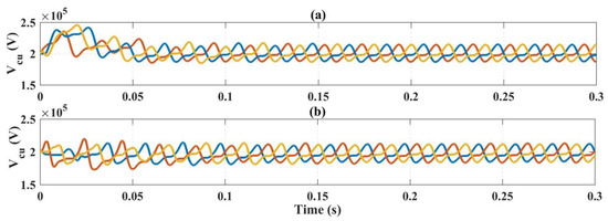
Figure 13.
Arm capacitor voltage; (a) control with SMC; (b) control with PR.
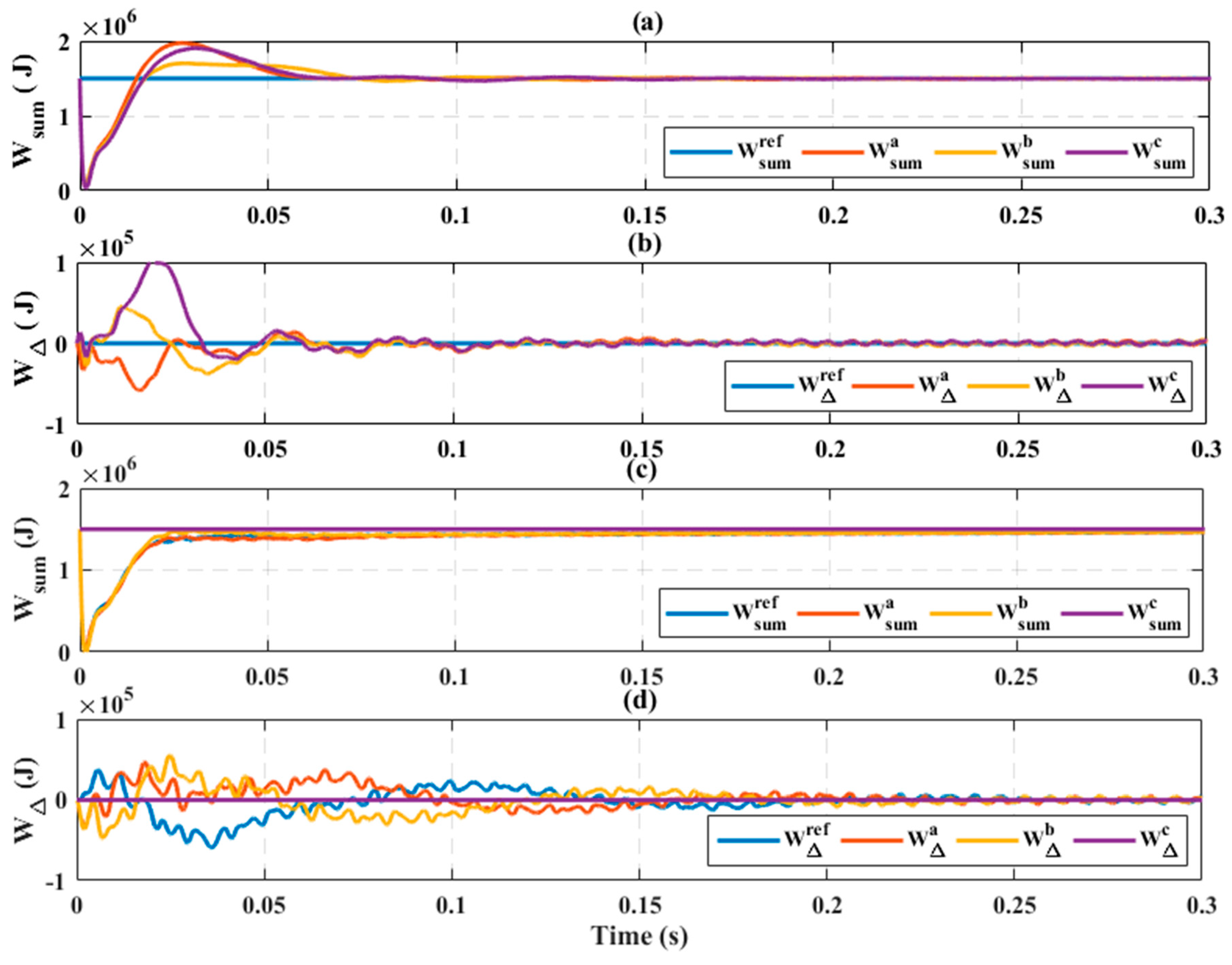
The energy sum and difference between the upper and lower arm are shown in Figure 14a–d. Figure 14a,b shows the responses of during use of the proposed controller while Figure 14c,d show the response of the PR controller.
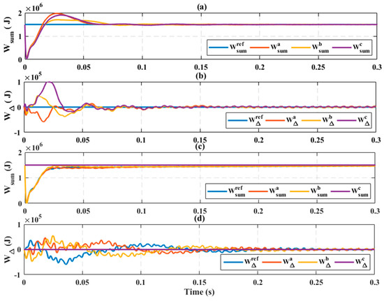
Figure 14.
(a) Energy sum control with SMC; (b) energy difference with SMC; (c) energy sum with PR; (d) energy difference with PR.
The energy sum is equal to the phase leg energy of MMC. The reference of is calculated from the equation . is SM voltage. The measured value of each arm is stabilized and follow the respective reference perfectly after . As SM capacitor voltage is responsible for energy storage, the regulated capacitor voltage results in a good and fast response of leg energy. After the initial charging of a capacitor, the response becomes well-regulated and follows the respective reference value. Similarly, Figure 14b depicts the energy difference between arms. Initially, due to the charging of the capacitor, there is a difference between an upper and lower arm of phase C but the controller tackles the problem and energy difference becomes zero afterward. The energy difference also ensures to track its reference value. The difference becomes zero at . This will cause both arms to reach equipotential and, hence, now charges will flow from one arm to another. However, in the case of PR, the measured leg energy reaches its reference value at , which shows a very slow response as compared to the proposed controller. Similarly, the energy difference becomes zero at , which also indicates a slow response. However, in steady-state, the PR controller tracks the reference energy difference signal.
Figure 15 depicts the output voltage of MMC. The output voltage has a good response to the proposed controller. The good response of output voltage is due to the well-regulated capacitor voltages of the upper arm and lower arm.
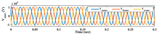
Figure 15.
Output voltage.
The results of the proposed controller and PR controller are shown in this section. SMC shows good encourageable performance as compared to PR. The attractive term in control law shows a good response, which is reflected in the result. The result shows that SMC has a fast dynamic response compared to PR. Moreover, in steady-state, it also minimizes the error, while in the case of the circulating current controller, the super-twisting algorithm has effectively suppressed second-order content in circulating current, resulting in a very small error as compared to PR.
Moreover, to have a clear picture and conclusion, the performance indices of both the controller are measured and represented in Table 1 and Table 2. The lower value of performance indices indicates good and stable control response.

Table 1.
Performance indices of output current controllers.
Table 2.
Performance indices of circulating current controllers.
Table 1 shows the performance indices of output current controller. In the case of , the integral square error (ISE) value of SMC controller is higher than PR controller. This is because the initial value of the sliding surface is zero while the initial value of is 1000 A. However, as the controller approaches its desired surface, it gives lower integral absolute error (IAE) and integral time absolute error (ITAE) values than the PR controller for . However, in the case of component of output current, SMC has lower values of ISE, IAE, and ITAE, which show the good response of controller.
Similarly, the performance indices for circulating current controllers are given in Table 2. By analyzing the value of all three-phase current, values of ISE, IAE, and ITAE are much smaller in the case of SMC compared to PR. As small values of performance indices shows best performance, it is concluded that SMC has a better response than PR in the case of circulating current.
5. Conclusions
This work is based on the current control of MMC using SMC design. Output and circulating current are controlled using separate controllers. The controller ensures the reference tracking of both output current and circulating current, and the second harmonics contents is well suppressed. Moreover, the proposed control scheme regulates capacitor arm voltages and the energy of system. The design of SMC-based control shows fast response in a transient state as well as in a steady state. The attractive term and equivalent terms in control law work very well. The measure value is attracted and steered on the reference value effectively. The design shows optimal performance of MMC parameters. The stability and robustness of controller is proved using Lyapunov analysis.
Author Contributions
W.U., K.Z., and M.I., proposed the main idea of the paper. W.U. implemented the mathematical derivations, simulation verifications, and analyses. The paper was written by W.U., and was revised by K.Z., M.I., S.u.I., M.A.K., and H.-J.K. All the authors were involved in preparing the final version of this manuscript. Furthermore, this whole work was supervised by H.-J.K., G.S.P., and C.L.
Funding
This research was supported by Basic Research Laboratory through the National Research Foundations of Korea funded by the Ministry of Science, ICT and Future Planning (NRF-2015R1A4A1041584).
Conflicts of Interest
The authors declare no conflict of Interest.
Nomenclature
| Acronym | Meaning | Units |
| Reference values | -- | |
| Equivalent and attractive terms | -- | |
| Three phases (abc) | -- | |
| upper arm and lower arm currents of phase | A | |
| , | output and circulating currents of phase | A |
| DC link voltage and current respectively | V, A | |
| 2nd harmonic of circulating current | A | |
| internal voltage of upper arm and lower arm | V | |
| Phase leg resistance and Inductance | ||
| Grid voltage | V | |
| , | Converter output and internal voltages respectively | V |
| Submodule capacitance | F | |
| Number of submodules in one arm | -- | |
| Submodule capacitor voltage | V | |
| sum of capacitor voltage of upper arm and lower arm | V | |
| insertion indices | -- | |
| active power | W | |
| number of phases | -- | |
| Sliding surface | -- | |
| control input | -- | |
| Quantity in three phase (abc), and systems respectively | -- | |
| angular frequency of grid voltage | ||
| Output voltage in dq-axis | V | |
| Grid voltage in dq-axis | V | |
| output current in dq-axis | A | |
| , , | Positive constant | -- |
| Lyapunov function | -- | |
| Energy sum and difference of both arms | J | |
| Signum function | -- | |
| State vector | -- | |
| , | nonlinear function of system state vector | -- |
| co-efficient of sliding function | ||
| Low pass filter | -- |
Appendix A
Transforming Equation (21) to stationary reference frame by using Clarke’s Transformation (), we get
Equation (A1) is solved for value given as
The switching function used in control law is given as
, and are positive and real numbers. The ful control law is given as
while
Appendix B
Table A1.
Converter Speciation.
Table A1.
Converter Speciation.
| Parameters | Value | Symbols | Units |
|---|---|---|---|
| D.C Voltage | 200 | kV | |
| Grid Voltage | 100 | kV | |
| Output Peak Current | 1 | kA | |
| Frequency | 50 | f | Hz |
| Number of level | 12 | N | - |
| Inducatnce | 50 | L | mH |
| Resistance | 1.57 | R | Ω |
| Capcitance | 0.45 | C | mF |
References
- Kouro, S.; Malinowski, M.; Gopakumar, K.; Pou, J.; Franquelo, L.G.; Bin, W.; Rodriguez, J.; Pérez, M.A.; Leon, J.I. Recent Advances and Industrial Applications of Multilevel Converters. IEEE Trans. Ind. Electron. 2010, 57, 2553–2580. [Google Scholar] [CrossRef]
- Perez, M.A.; Bernet, S.; Rodriguez, J.; Kouro, S.; Lizana, R. Circuit Topologies, Modeling, Control Schemes, and Applications of Modular Multilevel Converters. IEEE Trans. Power Electron. 2015, 30, 4–17. [Google Scholar] [CrossRef]
- Kolluri, S.; Gorla, N.B.Y.; Sapkota, R.; Panda, S.K. A new control approach for improved dynamic performance of MMC based HVDC subsea power transmission system. In Proceedings of the 2017 IEEE Innovative Smart Grid Technologies-Asia: Smart Grid for Smart Community (ISGT-Asia 2017), Auckland, New Zealand, 4–7 December 2017. [Google Scholar]
- Debnath, S.; Saeedifard, M. A New Hybrid Modular Multilevel Converter for Grid Connection of Large Wind Turbines. IEEE Trans. Sustain. Energy 2013, 4, 1051–1064. [Google Scholar] [CrossRef]
- Hagiwara, M.; Nishimura, K.; Akagi, H. A Medium-Voltage Motor Drive With a Modular Multilevel PWM Inverter. IEEE Trans. Power Electron. 2010, 25, 1786–1799. [Google Scholar] [CrossRef]
- Li, B.; Zhou, S.; Xu, D.; Yang, R.; Xu, D.; Buccella, C.; Cecati, C. An Improved Circulating Current Injection Method for Modular Multilevel Converters in Variable-Speed Drives. IEEE Trans. Ind. Electron. 2016, 63, 7215–7225. [Google Scholar] [CrossRef]
- Vasiladiotis, M.; Rufer, A. Analysis and control of modular multilevel converters with integrated battery energy storage. IEEE Trans. Power Electron. 2015, 30, 163–175. [Google Scholar] [CrossRef]
- Li, Y.; Han, Y. A Module-Integrated Distributed Battery Energy Storage and Management System. IEEE Trans. Power Electron. 2016, 31, 8260–8270. [Google Scholar] [CrossRef]
- Zeb, K.; Uddin, W.; Khan, M.A.; Ali, Z.; Ali, M.U.; Christofides, N.; Kim, H.J. A comprehensive review on inverter topologies and control strategies for grid connected photovoltaic system. Renew. Sustain. Energy Rev. 2018, 94, 1120–1141. [Google Scholar] [CrossRef]
- Nami, A.; Liang, J.; Dijkhuizen, F.; Demetriades, G.D. Modular Multilevel Converters for HVDC Applications: Review on Converter Cells and Functionalities. IEEE Trans. Power Electron. 2015, 30, 18–36. [Google Scholar] [CrossRef]
- Zeb, K.; Khan, I.; Uddin, W.; Khan, M.A.; Sathishkumar, P.; Busarello, T.D.C.; Ahmad, I.; Kim, H.J. A review on recent advances and future trends of transformerless inverter structures for single-phase grid-connected photovoltaic systems. Energies 2018, 11, 1968. [Google Scholar] [CrossRef]
- Ishfaq, M.; Uddin, W.; Zeb, K.; Khan, I.; Islam, S.U.; Khan, M.A.; Kim, H.J. A new adaptive approach to control circulating and output current of modular multilevel converter. Energies 2019, 12, 1118. [Google Scholar] [CrossRef]
- Hagiwara, M.; Akagi, H. Control and Experiment of Pulsewidth-Modulated Modular Multilevel Converters. IEEE Trans. Power Electron. 2009, 24, 1737–1746. [Google Scholar] [CrossRef]
- Lizana, R.; Perez, M.A.; Arancibia, D.; Espinoza, J.R.; Rodriguez, J. Decoupled Current Model and Control of Modular Multilevel Converters. IEEE Trans. Ind. Electron. 2015, 62, 5382–5392. [Google Scholar] [CrossRef]
- Riar, B.S.; Madawala, U.K. Decoupled control of modular multilevel converters using voltage correcting modules. IEEE Trans. Power Electron. 2015, 30, 690–698. [Google Scholar] [CrossRef]
- Bahrani, B.; Debnath, S.; Saeedifard, M. Circulating Current Suppression of the Modular Multilevel Converter in a Double-Frequency Rotating Reference Frame. IEEE Trans. Power Electron. 2016, 31, 783–792. [Google Scholar] [CrossRef]
- Qingrui, T.; Zheng, X.; Lie, X. Reduced Switching-Frequency Modulation and Circulating Current Suppression for Modular Multilevel Converters. IEEE Trans. Power Deliv. 2011, 26, 2009–2017. [Google Scholar] [CrossRef]
- Lacerda, V.A.; Coury, D.V.; Monaro, R.M. Proportional-Resonant controller applied to modular multilevel converter for HVDC systems. In Proceedings of the 2018 Simposio Brasileiro de Sistemas Eletricos (SBSE), Niteroi, Brazil, 12–16 May 2018; pp. 1–6. [Google Scholar]
- Li, S.; Wang, X.; Yao, Z.; Li, T.; Peng, Z. Circulating Current Suppressing Strategy for MMC-HVDC Based on Nonideal Proportional Resonant Controllers Under Unbalanced Grid Conditions. IEEE Trans. Power Electron. 2015, 30, 387–397. [Google Scholar] [CrossRef]
- He, L.; Zhang, K.; Xiong, J.; Fan, S. A Repetitive Control Scheme for Harmonic Suppression of Circulating Current in Modular Multilevel Converters. IEEE Trans. Power Electron. 2015, 30, 471–481. [Google Scholar] [CrossRef]
- Yang, S.; Wang, P.; Tang, Y.; Zagrodnik, M.; Hu, X.; Tseng, K.J. Circulating Current Suppression in Modular Multilevel Converters With Even-Harmonic Repetitive Control. IEEE Trans. Ind. Appl. 2018, 54, 298–309. [Google Scholar] [CrossRef]
- Yang, S.; Wang, P.; Tang, Y.; Zhang, L. Explicit Phase Lead Filter Design in Repetitive Control for Voltage Harmonic Mitigation of VSI-Based Islanded Microgrids. IEEE Trans. Ind. Electron. 2017, 64, 817–826. [Google Scholar] [CrossRef]
- Zhang, M.; Huang, L.; Yao, W.; Lu, Z. Circulating Harmonic Current Elimination of a CPS-PWM-Based Modular Multilevel Converter With a Plug-In Repetitive Controller. IEEE Trans. Power Electron. 2014, 29, 2083–2097. [Google Scholar] [CrossRef]
- Kolluri, S.; Gorla, N.B.Y.; Sapkota, R.; Panda, S.K. A New Control Architecture with Spatial Comb Filter and Spatial Repetitive Controller for Circulating Current Harmonics Elimination in a Droop Regulated Modular Multilevel Converter for Wind Farm Application. IEEE Trans. Power Electron. 2019, 34, 10509–10523. [Google Scholar] [CrossRef]
- Yang, Q.; Saeedifard, M.; Perez, M.A. Sliding Mode Control of the Modular Multilevel Converter. IEEE Trans. Ind. Electron. 2019, 66, 887–897. [Google Scholar] [CrossRef]
- Ishfaq, M.; Uddin, W.; Zeb, K.; Islam, S.U.; Hussain, S.; Khan, I.; Kim, H.J. Active and reactive power control of modular multilevel converter using sliding mode controller. In Proceedings of the 2019 2nd International Conference on Computing, Mathematics and Engineering Technologies (iCoMET 2019), Sukkur, Pakistan, 30–31 January 2019. [Google Scholar]
- Uddin, W.; Hussain, S.; Zeb, K.; Khalil, I.U.; Ullah, Z.; Dildar, M.A.; Adil, M.; Ishfaq, M.; Khan, I.; Kim, H.J. Effect of Arm Inductor on Harmonic Reduction in Modular Multilevel Converter. In Proceedings of the 4th International Conference on Power Generation Systems and Renewable Energy Technologies (PGSRET 2018), Islamabad, Pakistan, 10–12 September 2018. [Google Scholar]
- Din, W.U.; Zeb, K.; Ishfaq, M.; Islam, S.U.; Khan, I.; Kim, H.J. Control of internal dynamics of grid-connected modular multilevel converter using an integral backstepping controller. Electronics 2019, 8, 456. [Google Scholar] [CrossRef]
- Yang, S.; Wang, P.; Tang, Y. Feedback Linearization-Based Current Control Strategy for Modular Multilevel Converters. IEEE Trans. Power Electron. 2018, 33, 161–174. [Google Scholar] [CrossRef]
- Riar, B.S.; Geyer, T.; Madawala, U.K. Model Predictive Direct Current Control of Modular Multilevel Converters: Modeling, Analysis, and Experimental Evaluation. IEEE Trans. Power Electron. 2015, 30, 431–439. [Google Scholar] [CrossRef]
- Vatani, M.; Bahrani, B.; Saeedifard, M.; Hovd, M. Indirect Finite Control Set Model Predictive Control of Modular Multilevel Converters. IEEE Trans. Smart Grid 2015, 6, 1520–1529. [Google Scholar] [CrossRef]
- Dekka, A.; Wu, B.; Yaramasu, V.; Fuentes, R.L.; Zargari, N.R. Model Predictive Control of High-Power Modular Multilevel Converters—An Overview. IEEE J. Emerg. Sel. Top. Power Electron. 2019, 7, 168–183. [Google Scholar] [CrossRef]
- Bergna, G.; Garces, A.; Berne, E.; Egrot, P.; Arzande, A.; Vannier, J.-C.; Molinas, M. A Generalized Power Control Approach in ABC Frame for Modular Multilevel Converter HVDC Links Based on Mathematical Optimization. IEEE Trans. Power Deliv. 2014, 29, 386–394. [Google Scholar] [CrossRef]
- Gao, W.; Hung, J.C. Variable structure control of nonlinear systems: A new approach. IEEE Trans. Ind. Electron. 1993, 40, 45–55. [Google Scholar]
- Sharifabadi, K.; Harnefors, L.; Nee, H.-P.; Norrga, S.; Teodorescu, R. Dynamics and Control. In Design, Control and Application of Modular Multilevel Converters for HVDC Transmission Systems; John Wiley & Sons, Ltd.: Chichester, UK, 2016; pp. 133–213. [Google Scholar]
- Zeb, K.; Ayesha; Haider, A.; Uddin, W.; Qureshi, M.B.; Mehmood, C.A.; Jazlan, A.; Sreeram, V. Indirect Vector Control of Induction Motor using Adaptive Sliding Mode Controller. In Proceedings of the 2016 Australian Control Conference (AuCC), Newcastle, Australia, 3–4 November 2016; pp. 358–363. [Google Scholar]
- Zeb, K.; Uddin, W.; Khan, M.A.; Ayesha; Haider, A.; Kim, H.J. A comparative assessment of scalar controlled induction motor using PI, adaptive sliding mode, and FLC based on SD controllers. In Proceedings of the 2017 1st International Conference on Latest Trends in Electrical Engineering and Computing Technologies (INTELLECT 2017), Karachi, Pakistan, 15–16 November 2017. [Google Scholar]
- Zeb, K.; Din, W.; Khan, M.; Khan, A.; Younas, U.; Busarello, T.; Kim, H. Dynamic Simulations of Adaptive Design Approaches to Control the Speed of an Induction Machine Considering Parameter Uncertainties and External Perturbations. Energies 2018, 11, 2339. [Google Scholar] [CrossRef]
- Zeb, K.; Islam, S.U.; Din, W.U.; Khan, I.; Ishfaq, M.; Busarello, T.D.C.; Ahmad, I.; Kim, H.J. Design of fuzzy-PI and fuzzy-sliding mode controllers for single-phase two-stages grid- connected transformerless photovoltaic inverter. Electronics 2019, 8, 520. [Google Scholar] [CrossRef]
- Baghaee, H.R.; Mirsalim, M.; Gharehpetian, G.B.; Talebi, H.A. A Decentralized Power Management and Sliding Mode Control Strategy for Hybrid AC/DC Microgrids including Renewable Energy Resources. IEEE Trans. Ind. Inform. 2017. [Google Scholar] [CrossRef]
- Baghaee, H.R.; Mirsalim, M.; Gharehpetian, G.B.; Talebi, H.A. Decentralized Sliding Mode Control of WG/PV/FC Microgrids under Unbalanced and Nonlinear Load Conditions for On- and Off-Grid Modes. IEEE Syst. J. 2018, 12, 3108–3119. [Google Scholar] [CrossRef]
- Beltran, B.; Benbouzid, M.E.H.; Ahmed-Ali, T. Second-Order sliding mode control of a doubly fed induction generator driven wind turbine. IEEE Trans. Energy Convers. 2012, 27, 261–269. [Google Scholar] [CrossRef]
- Asad, M.; Ashraf, M.; Iqbal, S.; Bhatti, A.I. Chattering and stability analysis of the sliding mode control using inverse hyperbolic function. Int. J. Control. Autom. Syst. 2017, 15, 2608–2618. [Google Scholar] [CrossRef]
- Antonopoulos, A.; Angquist, L.; Nee, H.-P.P. On dynamics and voltage control of the Modular Multilevel Converter. In Proceedings of the 2009 13th European Conference on Power Electronics and Applications, Barcelona, Spain, 8–10 September 2009. [Google Scholar]


© 2019 by the authors. Licensee MDPI, Basel, Switzerland. This article is an open access article distributed under the terms and conditions of the Creative Commons Attribution (CC BY) license (http://creativecommons.org/licenses/by/4.0/).