Abstract
In this work the hydrodynamic performance of a novel wave energy converter configuration was analytically and numerically studied by combining a moonpool and a wave energy buoy, called the moonpool platform–wave energy buoy (MP–WEB). A potential flow, semi-analytical approach was adopted to assess the total (incident, diffraction, radiation) wave forces acting on the device, and the wave capture and energy efficiency performance of this configuration was assessed, both in the time and frequency domain. The performance of the two configurations, single float and double float, were analyzed and compared in terms of diffraction force, added mass radiation force, motion, and power in the frequency domain. Using an impulse response function-based (IRF) method, the frequency domain results were converted in the time domain. The same parameters in the time domain were derived and the main results were confirmed. Wave energy conversion efficiency was significantly increased due to the resonance phenomenon inside the moonpool.
1. Introduction
The interest in exploring marine renewable energy resources, including wind energy, tidal energy, and wave energy for power generation has steadily increased in the last ten years. Among the different kinds of marine energies, wave energy has become one of the most promising options. In recent years, the development and utilization of wind energy have been more extensive and the dynamic characteristics of wind turbines have become more mature. Current research is mainly focused on the signal control between wind farms and power grids. For example, Salah [1,2] used artificial neural network and multi-objective genetic algorithm to improve the performance of wind farm. Compared to the utilization of wind energy, the utilization of wave energy is still in the primary stage, and there is no corresponding research on the mechanism of hydrodynamic characteristics. Wave energy utilization technology is mainly through various forms of wave energy converter (WEC), to convert wave energy in sea water into electrical energy. The specific process is to convert wave energy into mechanical energy through conversion devices or equipment, and then convert mechanical energy into electrical energy, which is transmitted to the land through cables, and connected with the large power grid for users to use. As an energy conversion device, it can adapt to the wave conditions of the selected sea area, absorb wave energy in a stable and reliable manner, and realize energy conversion to the maximum extent. Wave energy converters (WECs) can be used to extract wave energy through the periodic resonance caused by slow-speed periodic waves. The oscillating bodies utilizing the heave motion can have small horizontal dimensions, compared to the incident wavelength. At the same time, this power generation principle can also be applied to single or multi-body point absorption WECS. Based on the same wave conversion principle, the typical single OBWEC (Oscillating Buoy WEC) is sea-based [3] developed by the Uppsala University in Sweden. The buoy is a relatively flat cylindrical type. The power take-off (PTO) is a linear motor, which is fixed on the seafloor by the gravity of the concrete pan. The float and PTO are connected by a flexible rope. A similar point suction wave energy device with a single buoy and a motion reference to the seafloor or other fixed structures is the fully submerged AWS (Archimedes wave swing) [4] in Portugal. The “CETO” [5] device developed by Carnege Australia and the Waveroller [6] swing device in Finland are arranged in a single array of OBWEC arrays, simultaneously interpreting the electrical energy between the devices.
The hydrodynamic characteristics of the absorber around it have a direct influence on the wave energy conversion efficiency. Several conceptual designs and studies of the absorber were carried out to improve the efficiency for extracting energy, theoretically and experimentally. Mavrakos and Katsaounis [7] investigated the different effects of floaters’ geometries by analyzing the performance of tight-moored, vertical axisymmetric WECs. The results showed the parametric effect of the varying hydrodynamic characteristics of each particular floater’s geometry on the investigated WECs’ performance characteristics. This kind of device was examined and comparatively assessed. Zang et al. [8] studied the power performance of a WEC with a heaving buoy and a power take-off (PTO) damping under regular and irregular waves. The capture width ratio in irregular waves was found to be approximately 5–40% higher than that in regular waves for the same wave parameters, although the absolute incident and absorbed wave power in irregular waves were only half of those in regular waves. Li and Yu [9] studied the hydrodynamic characteristics of the catamaran heave wave energy converter by using the RANS (Reynolds Average Navier-Stokes) method. The calculation result showed that the maximum wave absorbing efficiency of the device could reach 30% under the condition of buoy resonance. Falcão and Henriques [10] proposed a method of achieving sub-optimal phase-control. The method was based on the theoretical time domain modeling of a single-degree oscillating absorber in regular and irregular waves, by adequately delaying the release of the body. It was generally acknowledged that real sea conditions were irregular and random. However, there were fewer investigations about the hydrodynamic characteristics of oscillating wave energy converters in irregular waves. For example, Milani and Moghaddam [11] studied the process of controlling and maximizing the absorbed power of WECs under irregular waves; Bachynski et al. [12] promoted the superposition approach to calculate the response in irregular waves; and Yeung et al. [13] derived the hydrodynamic coefficient of a cylindrical float, and obtained the energy conversion efficiency of a power generation system by a model test. Compared to a single float converter, two-body wave energy converters could be applied into deeper ocean, which were not affected by the ocean depth and tide. Liang Changwei and Zuo lei [14] studied a two-body wave energy converter oscillating in heave, the dynamic of which was adopted by a linearized model in the frequency domain, with consideration of both the linear viscous damping and the hydrodynamic damping. Dai et al. [15] proposed a novel two-body floating wave energy converter (WEC), which was tested in the frequency domain to optimize the geometric and mechanical parameters, and subsequently, a time domain model was built for simulation of a multi- DOF (degree of freedom) motion system. This study developed a mathematical methodology to analyze the performance of a novel two-body WEC, composed of an inner cylindrical buoy and an outer toroidal-cylinder buoy. Wave power could be extracted by the relative heave motions between the inner and outer buoys. In order to solve the hydrodynamic problem of the two buoys, Cho and Kim [16] investigated the hydrodynamic performance of a two-body WEC through a systematic parametric study by using analytical solutions. Chen et al. [17] applied a semi-analytical method based on eigenfunction matching, in order to study the wave diffraction of cylindrical structures with a moonpool.
The traditional method can hardly explore the double floating body coupling resonance from the mechanism, and optimize the PTO damping to improve power efficient. Few research work has been done to analyze the motions of a system and the power absorbed by a converter under irregular waves. In this study, a semi-analytical method is applied to obtain the solution under the eigenfunction Expansion-Matching, highlighting the underpinning physics of the coupling resonance between two bodies, to maximize the energy extraction. The PTO damping was optimized to obtain a higher efficiency of wave energy conversion in the frequency domain research. By applying the IRF method, the coupled motion responses of the two floating bodies, such as MP–WEB used in this study, were also determined in the time domain. Finally, based on the ISSC (In-temational Ship Structure Conference) wave spectrum and the irregular wave simulation, the motion response and capture width ratio of the MP–WEB were investigated in irregular wave conditions.
2. Analytical Solution of MP–WEB in the Frequency Domain
Figure 1 shows the main fluid domain areas for the problem considered, where E represents the external fluid domain, B represents the fluid domain under the external body, M represents the moonpool fluid domain, and I represent the fluid domain under the central body. The radius and draft of the central body are , respectively; the inner and outer radius and draft of the external boy are , respectively, the depth of water is . The rectangular coordinate system and cylindrical coordinate system are used, the origin and -axis of the cylindrical coordinate system coincide with the rectangular coordinate system’s, in the -axis direction, the plane coincides with the undisturbed mean sea water level, the vertical -axis is positive upward and passes through the barycenter of the MP and the WEB. The following relations (see Equation (1)) can be used to convert the coordinates from the cylindrical to the orthogonal axis system.
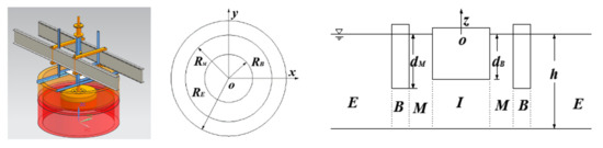
Figure 1.
Moonpool platform–wave energy buoy (MP–WEB).
2.1. Boundary Condition
To analyze the hydrodynamic characteristics of MP–WEB in the frequency domain, the analytical solution based on the series expansion of eigenfunctions is used to evaluate the velocity potentials. The velocity potential should be the solution of the Laplace equation (see Equation (2)) and should satisfy the following boundary conditions (see Equations (3)–(5)). In addition, a radiation condition must be satisfied (Equation (6))
Laplace’s equation:
Free surface condition:
Seabed condition:
Hull boundary condition:
Radiation condition:
where, is the acceleration of gravity, is the imaginary unit, and is the wave number obtained from the dispersion relation, and the symbol indicates that the derivation in the normal vector always points outwards from the wetted surface of the device.
2.2. Wave Force
The whole wet surface can be divided into four fluid subdomains (Figure 1); they are listed as follows:
- Fluid subdomain , whose diffraction and radiation velocity potential are and respectively;
- Fluid subdomain , whose diffraction and radiation velocity potential are and respectively;
- Fluid subdomain , whose diffraction and radiation velocity potential are and respectively;
- Fluid subdomain , whose diffraction and radiation velocity potential are and respectively.
The velocity potential of diffraction wave can be expressed as
According to the analytical-numerical method based on potential flow theory, using variables separation, the diffraction velocity potential in each subdomain can be obtained based on the boundary conditions, as follows:
where is the Bessel function of the third kind, which can be indicated as , and are the second and third kind of Bessel function, respectively, is the first kind of Bessel function, both (, , , , ) and (, , , , ) are unknown Fourier coefficients, which can be gained by boundary continuity conditions of an adjacent watershed; in addition
Apart from the series expression of diffraction velocity potential in each subdomain, the above unknown Fourier coefficients impose the continuity of the velocity potential and its derivative at the interface between two subdomains, as follows:
Additionally, according to the non-penetration conditions, the derivative of velocity potential must satisfy the following conditions:
In order to satisfy the velocity potential continuity condition at the coupling interface, the system of integral equations can be obtained by using the Galerkin method and the orthogonality of function
In order to satisfy the continuity condition of the derivative of velocity potential at the coupling interface, while at the same time considering the surface condition at the cylindrical surface, the integral function can be obtained by using the Galerkin method and the orthogonality of function
Solving the system of linear equations formed by Equations (25)–(30), the unknown Fourier coefficients could be determined in each subdomain, and therefore, the analytical expression could be obtained in each subdomain. Based on the Bernoulli equation, the wave excitation force in the vertical direction could be obtained by using the top and bottom surface velocity potential
where subscripts B and M, respectively, represent WEB and MP.
2.3. Added Mass and Damping Coefficients
When a small oscillation occurred, the structure would produce a radiated wave field outwards, acting on the floating bodies. Separating the radiated wave load, velocity, and acceleration, the added mass and radiation damping coefficients were obtained. The velocity potential of the heaving motion could be expressed as follows:
The radiation velocity potential satisfied the Laplace function, the linear free surface condition, the seabed condition, and the infinite radiation condition. The radiation velocity potential in each subdomain could be expressed as:
where the specific expression of , , and are shown in Equations (12)–(19). The particular solution of radiation velocity in each subdomain could be written as:
Similar to the diffraction problem, in order to derive the unknown Fourier coefficients in the series expressions of the radiation velocity potential, the continuity condition of the velocity potential and its derivative in the flow field interface were imposed, as follows:
Furthermore, imposing the non-penetration condition on the wet surfaces, the following expressions were obtained:
The following integral equation could be obtained by using the Galerkin method and orthogonal property of the function:
Considering the surface condition on the cylindrical surface, using the Galerkin method and the orthogonal property of the function, we have:
According to the integral Equations (48)–(50), the linear system of equations could be obtained, which could be used to derive the unknown Fourier coefficients resulting from the small amplitude motion in heave of the MP and the WEB in each subdomain, so that the series expression of radiation velocity potential could be obtained. According to the Bernoulli integral function, the radiation force in the vertical direction could be obtained, which could be expressed as:
where the and represent added mass and radiation damping, respectively, subscripts , , , and represent the impact of the MP on itself, impact of the MP on the WEB, impact of the WEB on the MP, and impact of the WEB on itself, respectively.
2.4. Dynamic Characteristic in The Frequency Domain
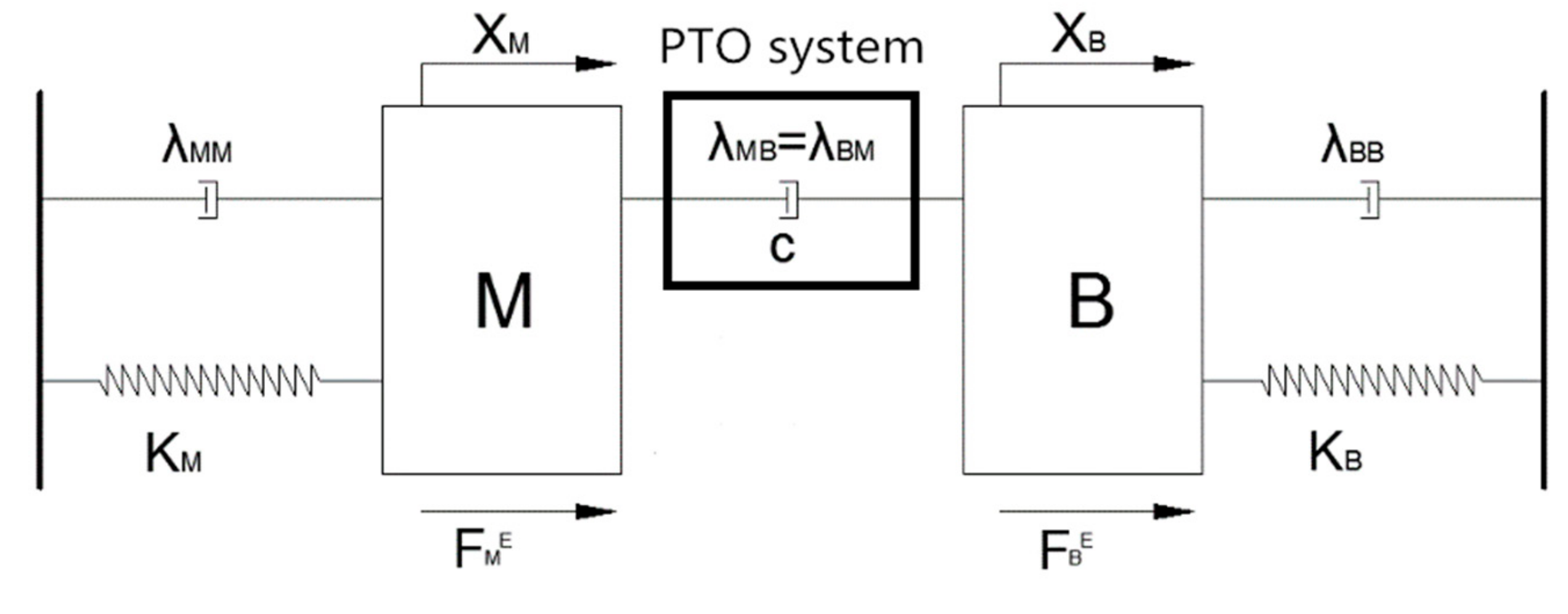
Based on the semi-analytical method of the eigenfunction expansion and the boundary conditions, the velocity potential expression around the MP–WEB was derived, so that the wave load and the hydrodynamic coefficient of the internal and external bodies could be obtained. To evaluate the wave energy conversion efficiency, the whole system (representing the WEB, the MP, and the PTO connecting them) was represented as a forced damped vibration system with two degrees of freedom under the wave action, as shown in Figure 2.
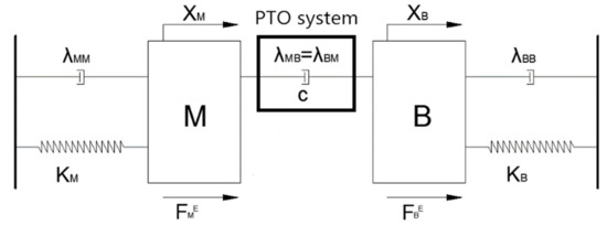
Figure 2.
Two degrees of freedom vibration system in the vertical direction.
Assuming that the dual system meets the static balance in calm water, the displacement is expressed as the relative displacement between the instantaneous position and equilibrium position. A linear, small-amplitude wave hypothesis was assumed. According to Newton’s second law, the motion equation of the forced vibration system could be expressed as
where represent the mass of the MP and the WEB, respectively; represent the displacement related to the hydrostatic equilibrium of the MP and the WEB, respectively; represent the wave load of the MP and the WEB, respectively, represent the radiation force of the MP on itself, the radiation force of the MP on the WEB, the radiation force of the WEB on itself, respectively, and the radiation force of the WEB on the MP, which could be written as:
represent the hydrostatic restoring force of the MP and the WEB, respectively, which could be expressed as
where represent static water restoring the force stiffness of the MP and the WEB, respectively, when the waterline area of the floating body is constant, which could be expressed as , where and are the sea water density and gravitational acceleration, respectively. is the PTO force, which could be expressed as the damping force associated with the relative velocity between the two bodies, as follows:
Assuming that the damping coefficient is linear, by substituting Equations (56)–(58) into Equation (55), the equations of motion for the MP–WEB system could be written as:
The equations of motion in the frequency domain could be obtained as follows:
The MP and the WEB are connected through the PTO system; under the wave loading, the relative motion between the MP and the WEB is damped by the PTO system, producing a power that could be expressed as:
Substituting Equation (58) into Equation (61)
where is incident frequency, represent the motion amplitude of the MP and the WEB, and is the PTO damping coefficient.
On account of the buoy configuration or size on wave energy conversion, it is no longer possible to measure the effect of the buoy configuration by just comparing the converted power, so the capture width radio could be applied to overlook that of the effect.
The capture width ratio represents the average output power to wave input power within the float width ratio, represented by the letter . The incident wave velocity potential, in Cartesian coordinates, with amplitude , frequency , and phase angle , is:
where the wave number satisfies the dispersion relation.
According to the Bernoulli equation, the input energy within one period, over the 2R width could be expressed as
Substituting Equations (63) in Equation (64):
The dispersion relation was substituted into the Equation (65)
The capture width ratio could be expressed as:
2.5. Optimize Power Take Off (OPT)
The design optimization of the converter should be regarded as a preliminary task. As the power performance of the WEC depends on the body geometry and the PTO parameters, the design optimization is a difficult task to complete.
According to the motion response equation in the frequency domain, the PTO coefficient could be defined as a variate. According to Equation (60), and could be written as
where
, , , and are all complex variable functions.
and can be subtracted from the Equation (68)
is a plural version.
The formula could be written as
In order to know the maximum of by taking the value of
According to Equations (75) and (76), this could be written as
Solving Equation (77), the optimal PTO damping coefficient is
3. Dynamic Characteristic Analyses of the MP–WEB in Frequency Domain Analysis
3.1. Verification for the Solution Method
In order to verify the present semi-analytical method, comparisons between the present method and the numerical method implemented in HydroStar (a software developed by Bureau Veritas) for fixed design parameters (, ) are shown in Table 1. Table 1 shows the comparison between the wave forces and the hydrodynamic coefficients in heave, calculated by the present method and the numerical method. The numerical results show a high agreement, which could be regarded as a validation of the present method. The total results are dimensionless.

Table 1.
Verification of the solution method.
3.2. Wave Force
For a wave energy buoy with a cylindrical moonpool platform in shallow water, recalling Equation (32), the non-dimensional wave force could be written as:
where the water depth is , the sea-water density , the gravitational acceleration , the wave amplitude , and the wave frequency range considered is . A parametric analysis was conducted by varying the dimensions of the MP, and keeping the geometry of the WEB fixed. The WEB radius was and its draft . Meanwhile, the difference between the outer and the inner diameter of the moon pool was kept fixed to reduce the research variables. The inner radius of the MP varied from , , , to , the draft of the MP varied from , , , to .
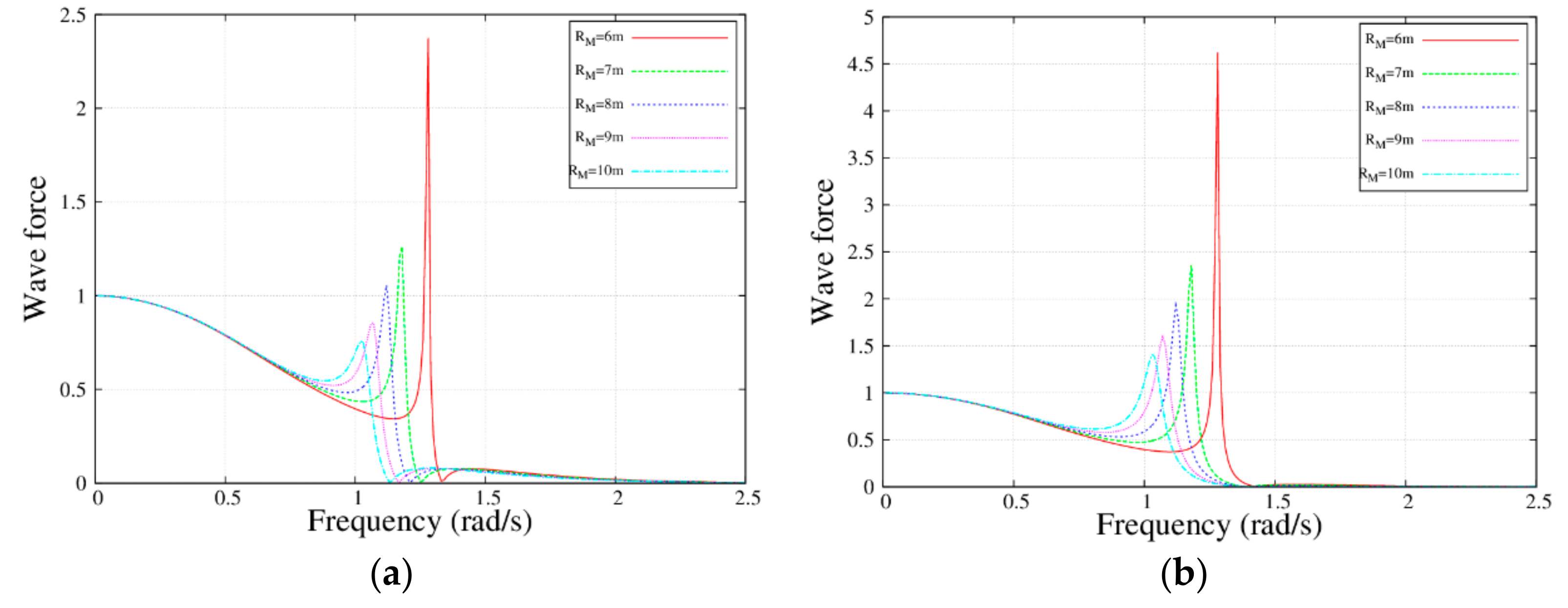
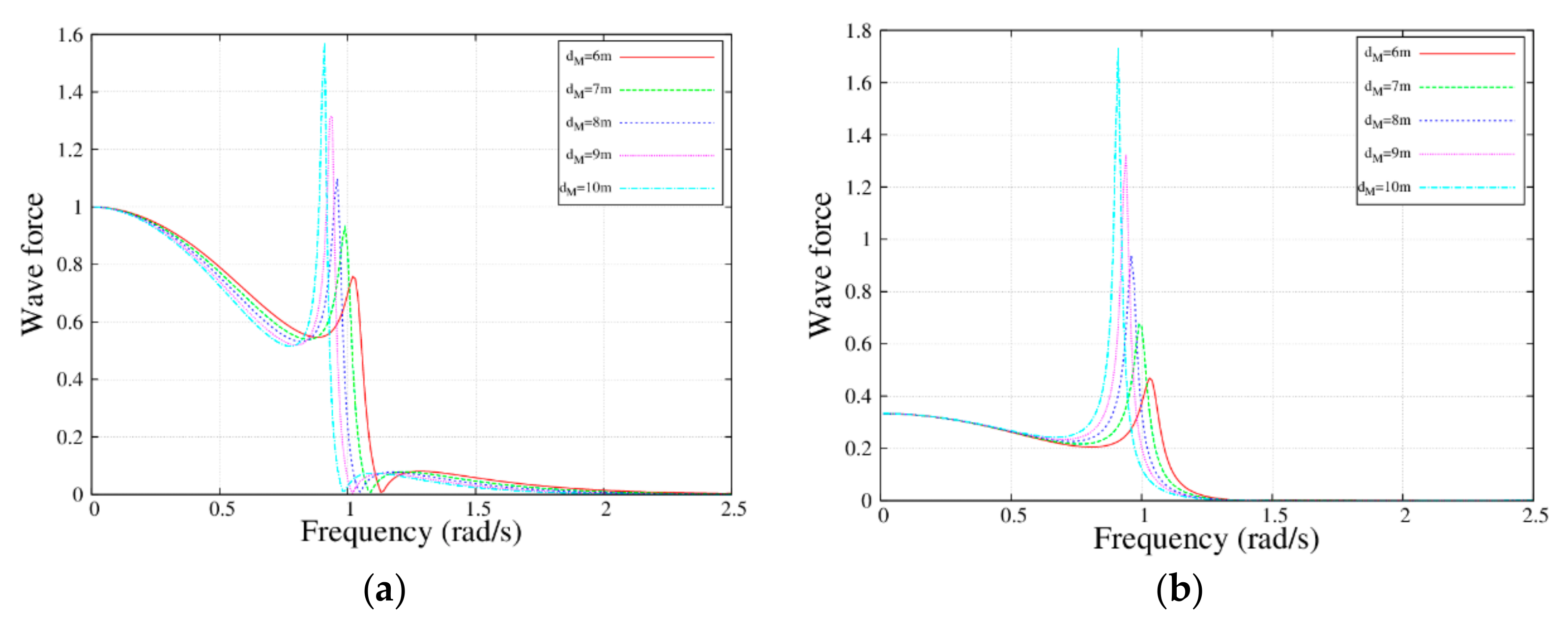
Figure 3 and Figure 4 show the wave force of the MP and the WEB for varying radius and draft. It could be seen that the wave force was reduced at the peak frequency with an increase in the radius of the MP. Furthermore, the peak frequency had a uniform trend at the same time. In contrast, the wave force was increased by increasing the draft. Moreover, for the same MP dimension, the wave load on the WEB was higher than that of the MP because of the different radiation effect, as the moonpool had a more radiated force on the buoy. In such a case, we could conclude that both the MP and the WEB would receive more wave force for the slender MP, but the stubbed MP had the opposite result.
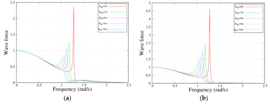
Figure 3.
Wave load with the frequency for the MP and the WEB with different radius; , , , and . (a) ; and (b) .
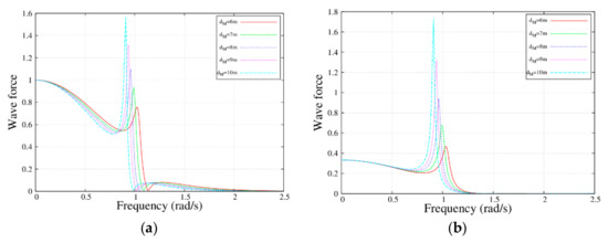
Figure 4.
Wave load with the frequency for the MP and the WEB with different draft; , , , and . (a) ; and (b) .
3.3. Added Mass and Damping Coefficients
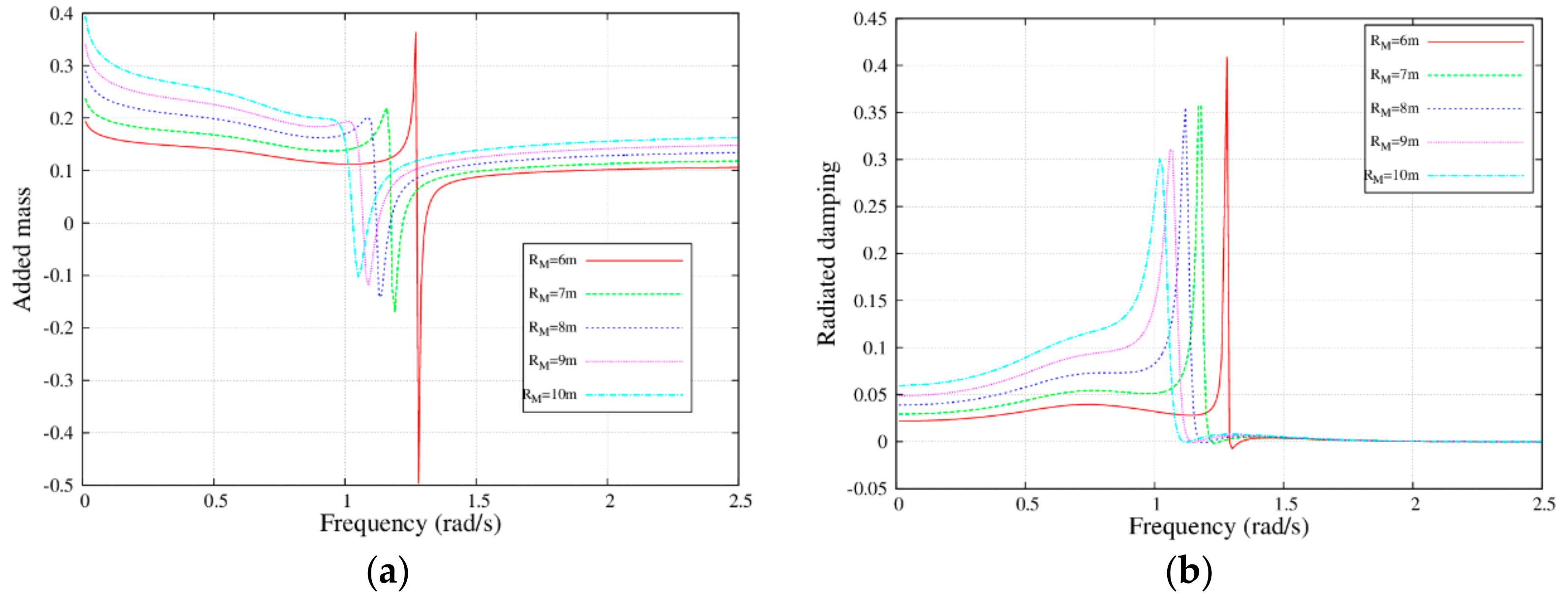
In this section, the influence of the draft dM and radius RM on the added mass and damping coefficients was investigated, using Equations (51)–(54). The dimensionless added mass and damping coefficients could be expressed as:
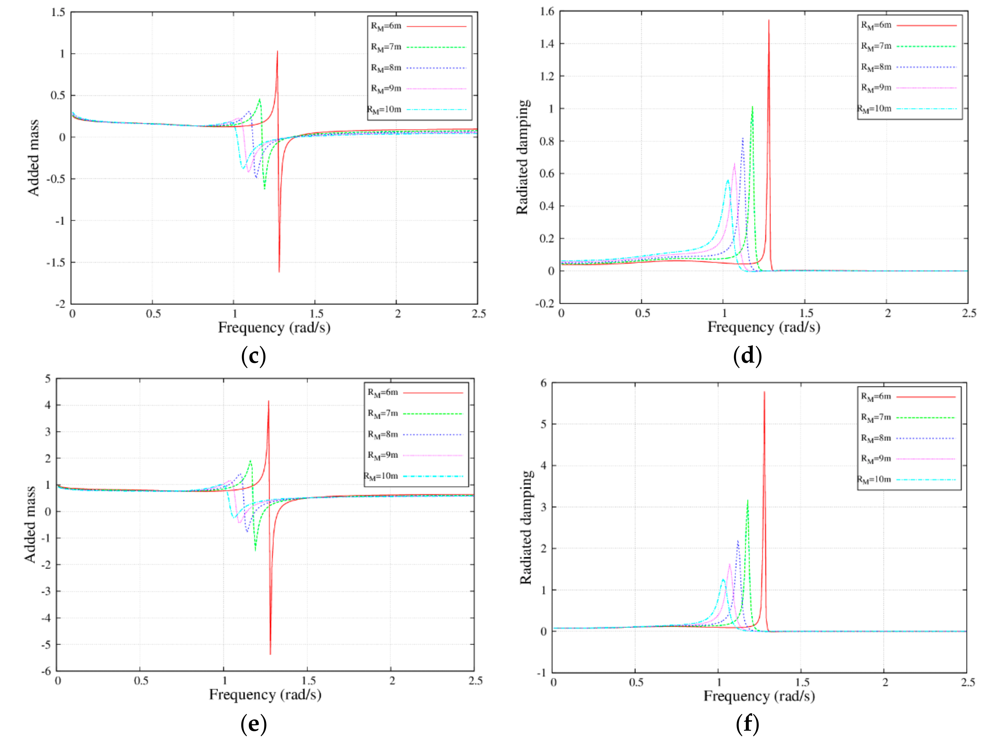
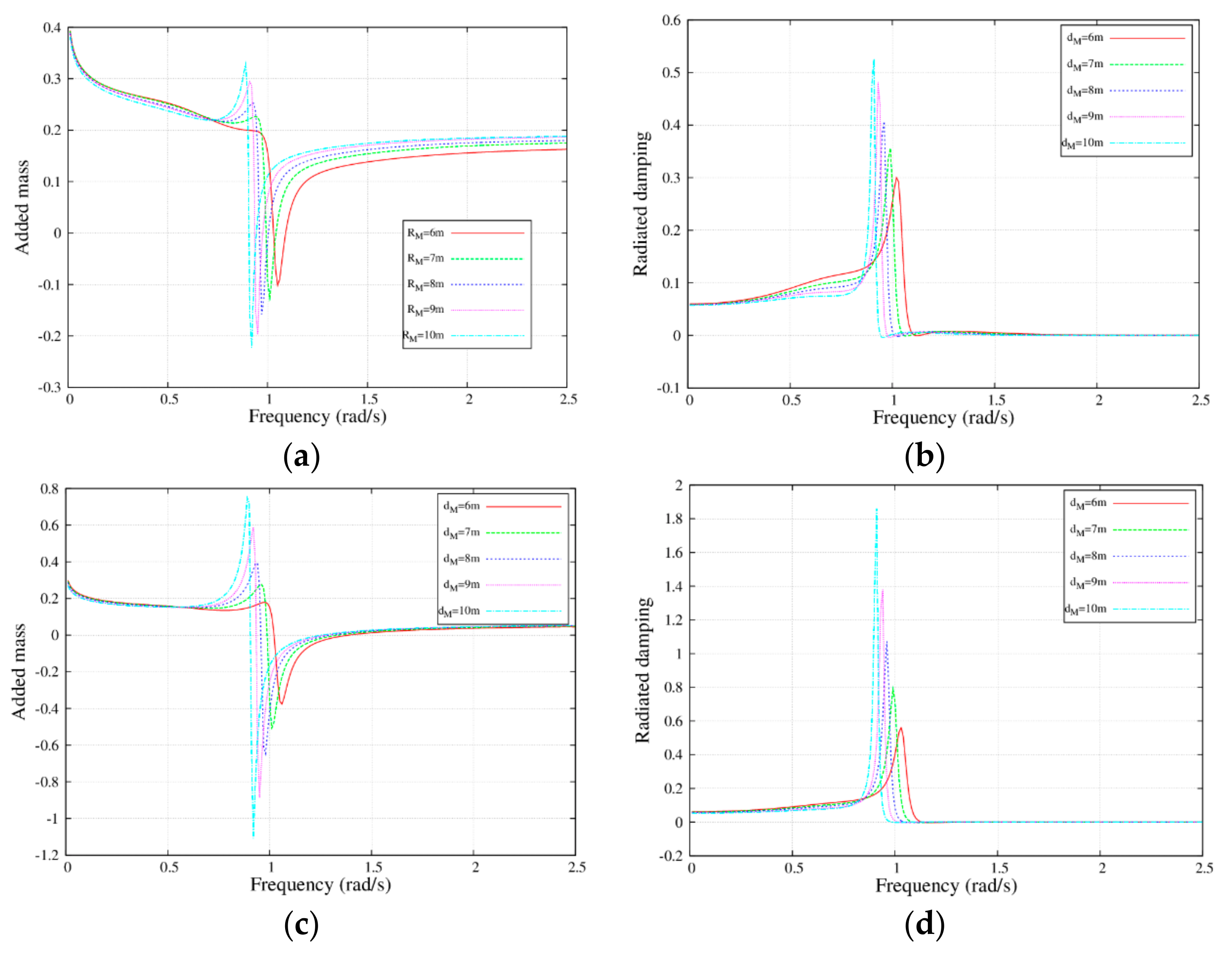
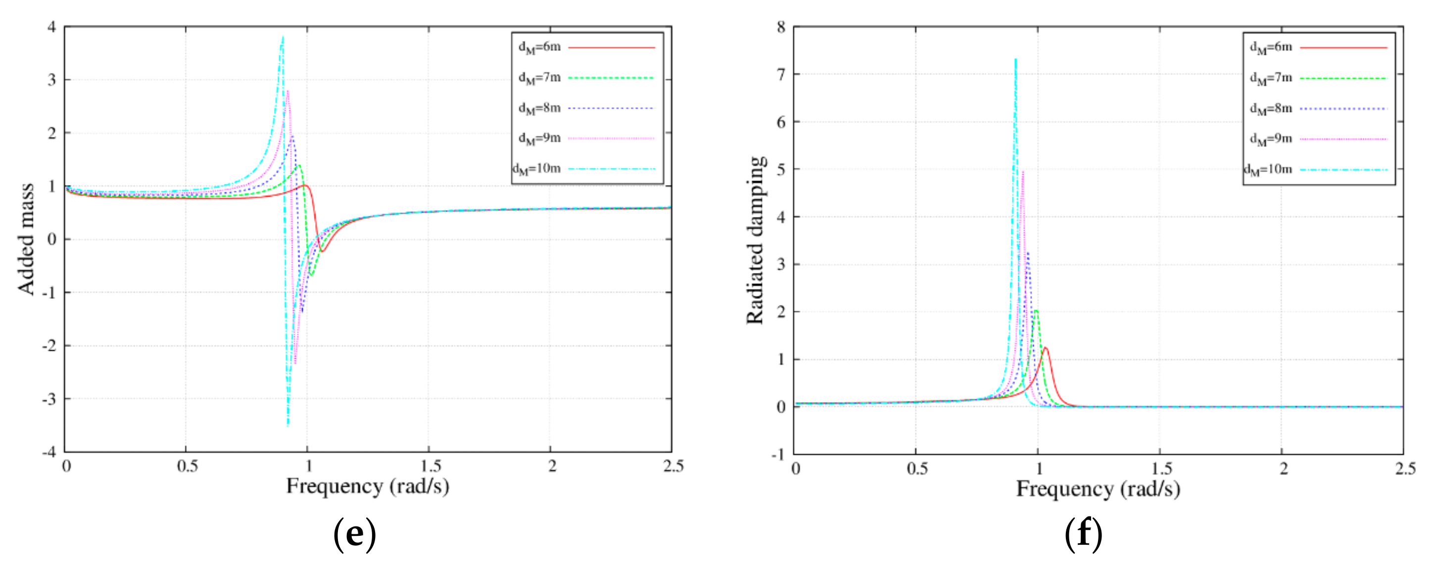
Figure 5 and Figure 6 show the added mass and radiation damping with different radius and draft for the MP. It was found that there were two peaks, i.e., one positive and one negative, for added mass in the frequency range of rad/s, but only one peak for radiation damping. The absolute peak values of the added mass were reduced with increasing radius, and the radiated damping showed the same trend. In addition, the peak frequency of the added mass was equal to that of the radiated damping.
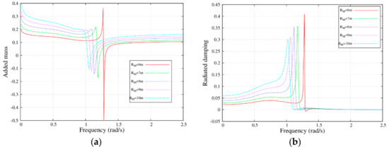
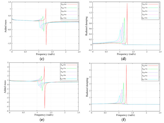
Figure 5.
Added mass and damping coefficients with the frequency for MM (MP to MP), MB (MP to WEB or WEB to MP), and BB (WEB to WEB) with different draft; , , , , and . (a) ; (b) ; (c) ; (d) ; (e) ; and (f) .
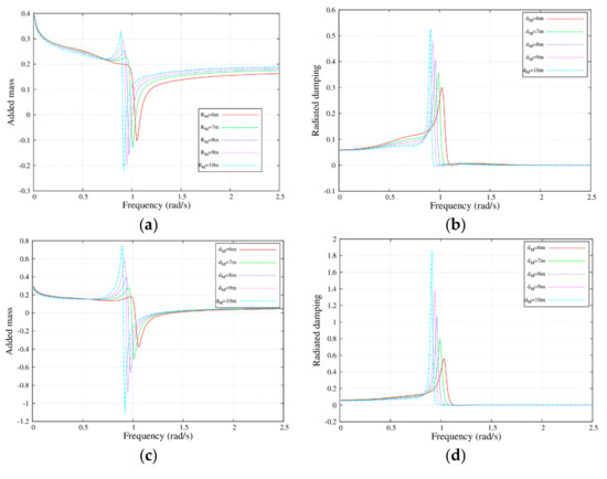
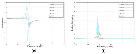
Figure 6.
Added mass and damping coefficients with the frequency for MM, MB, and BB with different draft; , , , , and .(a) ; (b) ; (c) ; (d) ; (e) ; and (f) .
3.4. Response Amplitude Operator (RAO)
The results of the RAO were given by Equation (60), which could be used to verify the influence of the geometrical parameter of the MP and PTO damping coefficients on the WEB motion.
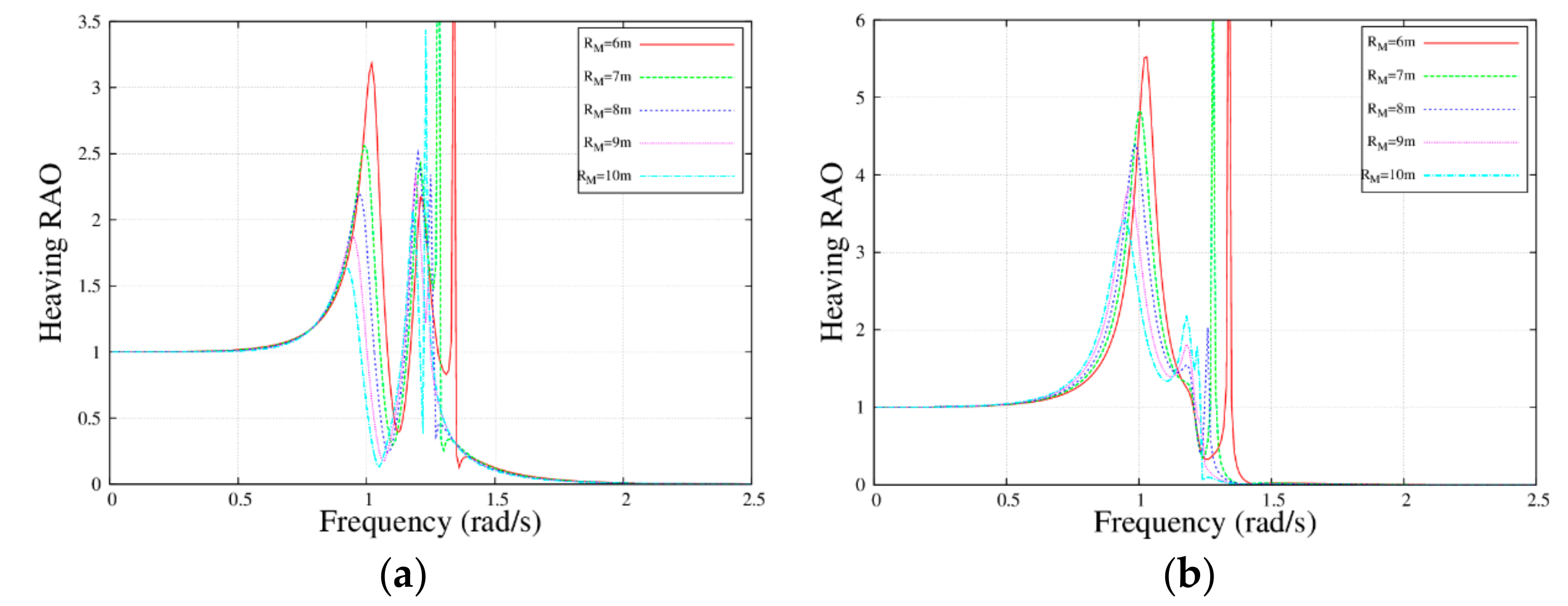
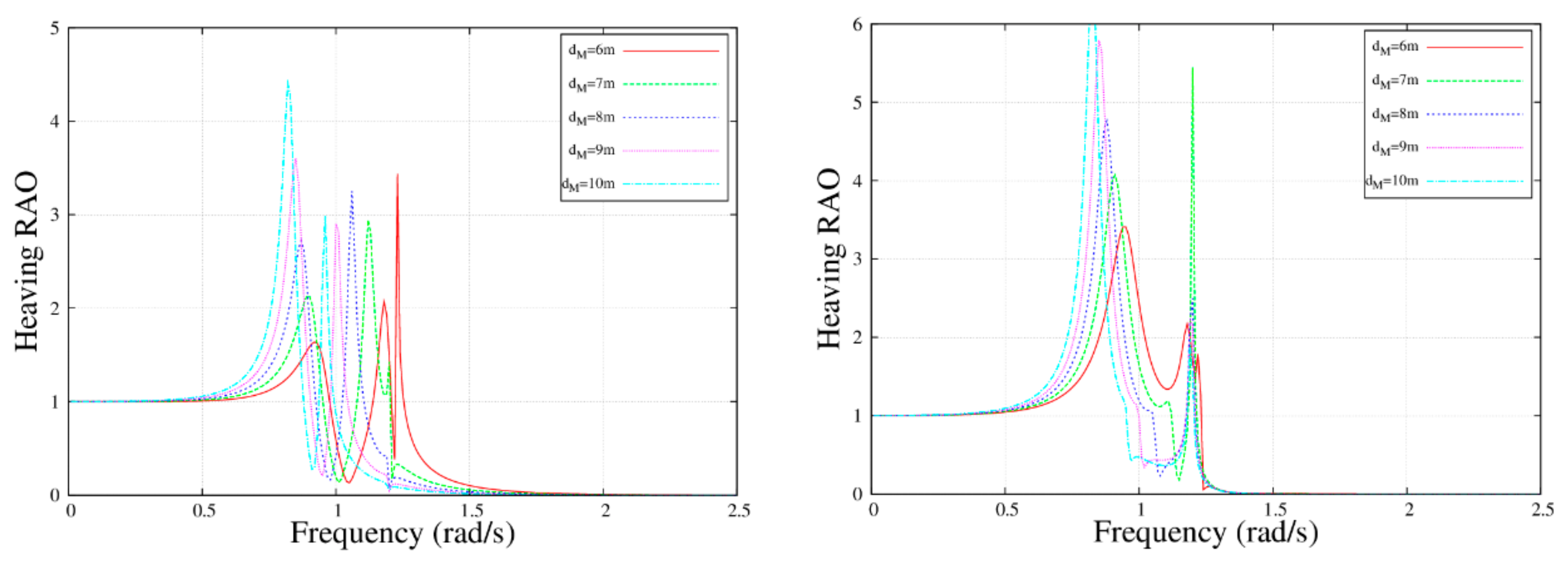
Figure 7 and Figure 8 depict the motion response for the MP–WEB with different MP dimensions (RM and dM). Here, we can clearly find three peaks in the figure. The first peak was due to the natural frequency of the WEB itself, the second peak was due to the natural frequency of the water column within the MP, and the third peak was due to the natural frequency of the MP itself. When these natural frequencies were close to the incident wave frequencies, resonance would occur. When the draft of the MP remained unchanged, the motion response of the MP and the WEB decreased as the radius increased. However, the draft of the MP presented an opposite trend. In short, the slender MP had a more pronounced motion response than that of the stubby MP.
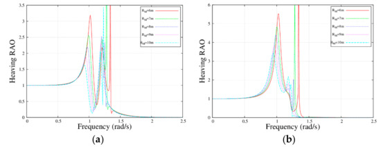
Figure 7.
Response amplitude operator with the frequency for the MP and the WEB with different radius; , , , , and . (a) and (b) .
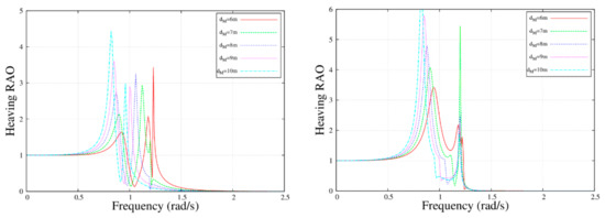
Figure 8.
Response amplitude operator with the frequency for the MP and the WEB with different draft; , , , , and . (a) ; and (b) .
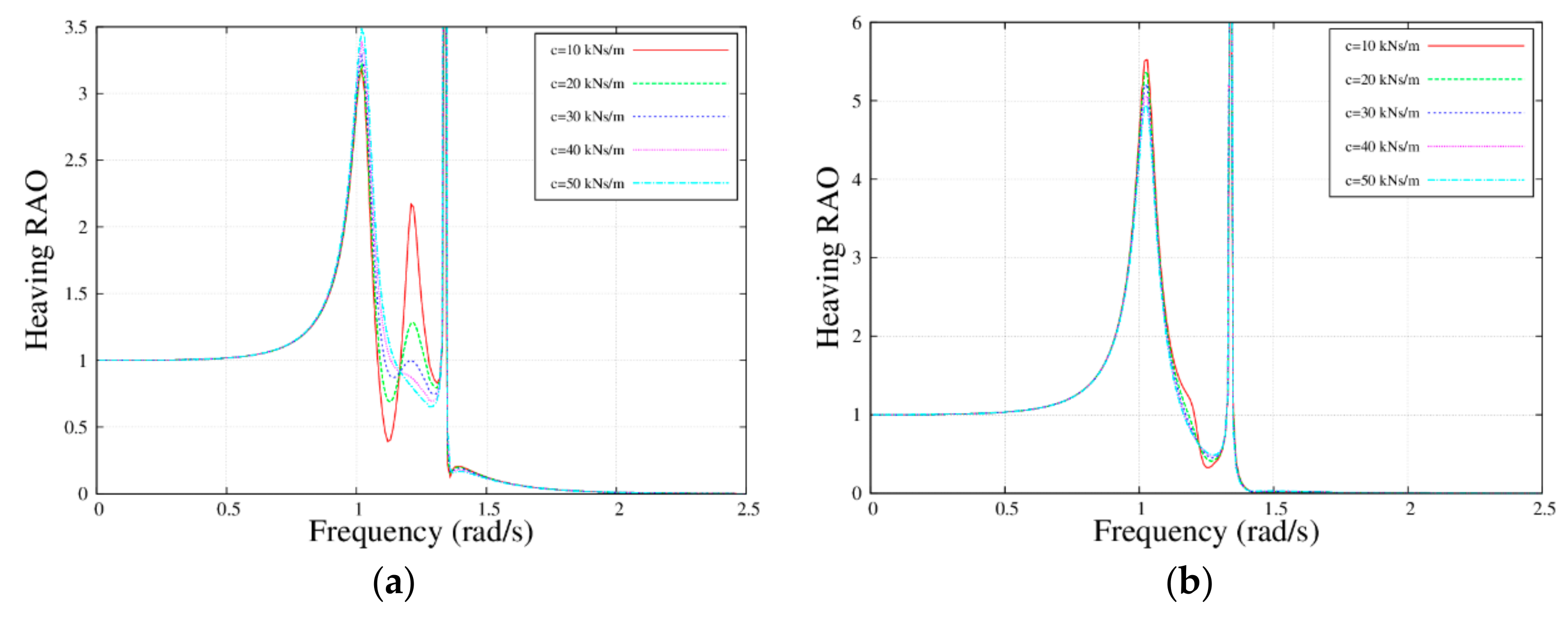
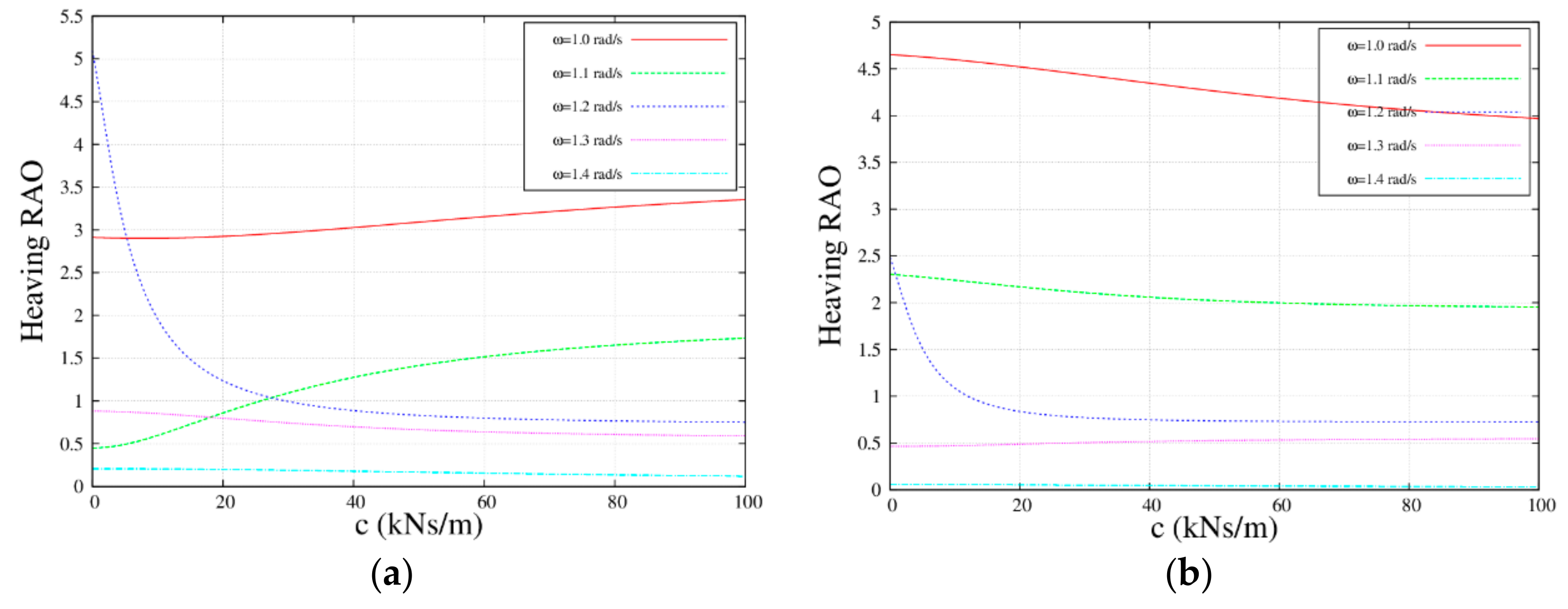
Based upon the former calculations, the optimum MP dimension could be obtained, i.e., an MP with a radius and a draft , while the dimensions of the WEB and the wave condition remained unchanged. Figure 8 showed the motion response for the MP and the WEB with various PTO damping coefficients , , , , and , and at various frequencies , , , , and , respectively.
Figure 9 and Figure 10 illustrate the influence of the PTO damping coefficient on the motion response. Clearly, the damping coefficient affected the peak value but not the peak frequency. The first and third peaks had the same trend, but that of the MP was opposite to the WEB’s. The reason was that the motion response of the WEB was greater than the motion response of the MP, and the PTO damping system had a negative effect on the WEB, so that its peak value was reduced with increasing PTO damping coefficients. In contrast, the PTO damping system had a positive effect on the MP, and its peak value was increased with increasing PTO damping. The motion response of the MP was reduced at frequencies and , while it was increased at the frequency , , and , while the WEB presented an opposite trend.
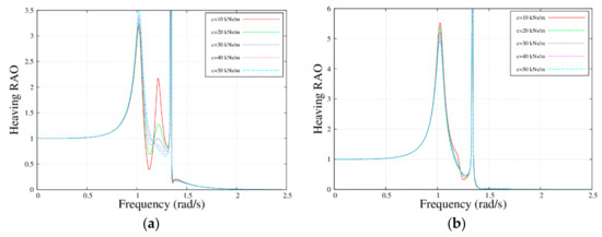
Figure 9.
Response amplitude operator with the frequency for the MP and the WEB with different power take-off (PTO) damping coefficients; , , , , and . (a) ; and (b) .
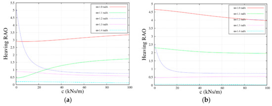
Figure 10.
Response amplitude operator with the PTO damping coefficient for the MP and the WEB with different frequencies; , , , , and . (a) ; and (b) .
3.5. Capture Width Ratio
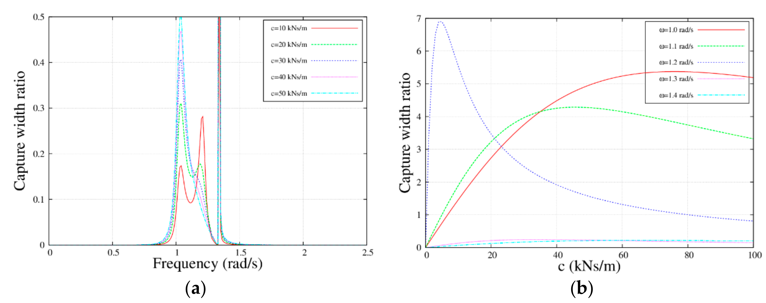
The previous section verified the effect of the MP on the RAO, so the influence on the capture width ratio was also explored and obtained according to Equation (67).
The left figure (a) in Figure 11 depicts the capture width ratios for the MP, parametrized against the PTO damping coefficient, for the following range of values: , , , , and . The capture width ratios for the MP with frequency , , , , and are illustrated, respectively, in the right figure. It can be seen that there were three peaks in the left figure, all of which were caused by the resonant frequency. The first and third peak values increased as the PTO damping coefficient decreased. Furthermore, another important conclusion obtained from the two graphs was that the capture width ratio highly depended on the PTO damping coefficients and first increased and then decreased as the PTO damping coefficients increased. Of most importance was that when the frequency approached , the optimal PTO damping coefficient was minimal.

Figure 11.
Capture width ratio with the PTO damping coefficient and frequency for the MP–WEB, , , , , and ; , , , , and (a) Capture width ratio in different PTO damping coefficient; and (b) capture width ratio in different frequencies.
4. An Analytical-Numerical Solution of MP–WEB in Time Domain Analysis
4.1. Motion Response
The time domain motion equation could be written as:
where represent the mass of the MP and WEB, respectively; represent the hydrostatic stiffness coefficient; is the added mass at infinite frequency, is the retardation function, where the subscripts represent influence of the MP on itself, influence of the MP on WEB, influence of the WEB on the MP, and influence of the WEB on itself, respectively. represent the instantaneous PTO force acting on the MP and WEB, which could be written as:
In order to transform the time domain kinematic formula of the MP–WEB, Equation (82) was defined as
The first order differential system could be obtained by substituting Equation (84) into Equation (82)
Equation (85) was solved using the Runge–Kutta integration method of the fourth order.
4.2. Instantaneous Capture Width Ratio
The instantaneous PTO damping system power could be expressed as:
substituting Equation (87) into Equation (86),
The incident wave velocity potential, with amplitude , frequency , and phase angle , could be written as in the rectangular coordinate system
where wave number satisfies the dispersion relations, so according to the Bernoulli function the input energy per period and float width could be expressed as
Combining Equations (88) and (89),
The dispersion relation was further substituted into Equation (90)
Thus, we could obtain instantaneous capture width ratio with frequency in the regular wave
4.3. Irregular Wave Simulation
For irregular waves, the diffraction wave force could be written as
where
Considering the ISSC spectrum,
where expresses significant wave height and expresses the spectral peak period.
Under linear theory, the velocity potential of incident waves could be expressed as the superposition of several velocity potentials in regular waves, which could be specifically expressed as
Assuming that the energy spectrum function of irregular waves is , the input energy of the incident wave per unit width in this sea condition could be expressed as
where represents the amplitude of incident wave under frequency and represents the random phase. Thus, what we could obtain is that from the capture width ratio in the irregular waves whose significant wave height is and spectral peak period is ,
5. Dynamics of the MP–WEB in Time Domain Analysis
5.1. Motion Response in Regular Waves
In this section, the MP–WEB is introduced and explored using the same analytical solution method according to Equation (85). The influencing factors of the MP on the WEB could be summarized as submerged depth, radius, height, and thickness for the MP, water depth, as well as the PTO damping coefficients. To eliminate the influences of the MP and the WEB geometry, the radius and draft of the WEB were kept fixed at . Meanwhile, the radius and draft of the MP were all the same with and the thickness was . In addition, the water depth and PTO damping coefficients were all the same with and .
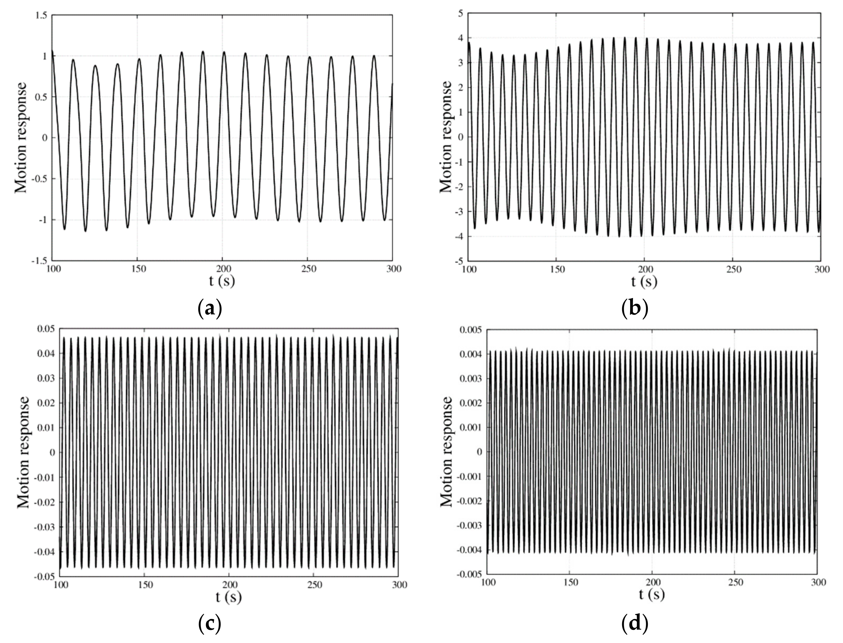
Figure 12 illustrates the time domain motion response of the MP–WEB with different frequencies. The frequencies of incident waves are , , , and , respectively. At first, the numerical results for the relative motion between the MP and the WEB appear to show transient variation; the curve changes periodically as time goes on. Furthermore, the steady peaks are highly dependent on the frequency; when the frequencies are , , , and respectively, the amplitude values of the time domain motion response are , , , and , respectively, all of which are close to the results of the frequency domain as shown in Table 2.
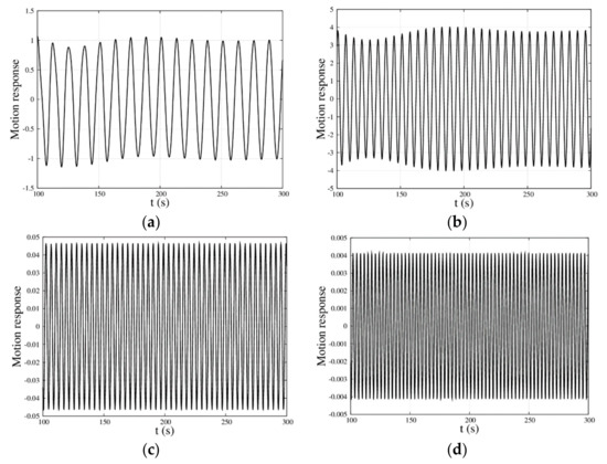
Figure 12.
Motion response with time for the MP–WEB with different frequency; , , , and . (a) ; (b) ; (c) ; and (d) .
Table 2.
The comparison between the motion response results of the frequency domain and time domain (m).
5.2. Instantaneous Capture Width Ratio in Regular Waves
According to Equation (92), the different frequencies could be applied to obtain the capture width ratio over time. In addition, the equipment parameters were the same as above.
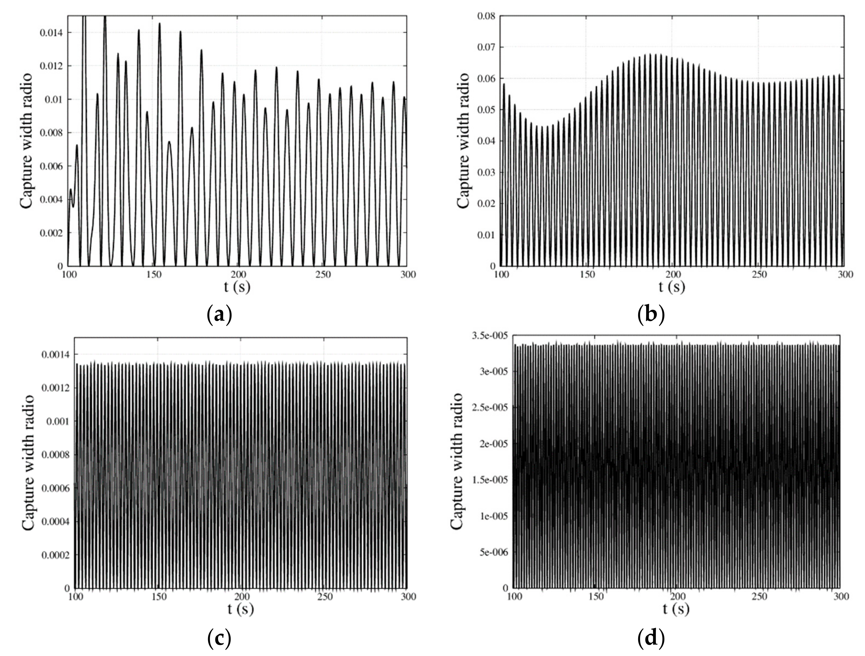
The capture width ratios for the various frequencies , , , and , respectively, are shown in Figure 13. From the figure, it was found that different from the changing curve of motion response, the curve of capture width ratio was above the coordinate axis, but what was same was that the curve changed periodically, as time went on. Furthermore, when the frequencies were , , , and , the amplitude values of the capture width ratios were , , , and , respectively, all of which were close to the results of the frequency domain as shown in Table 3.
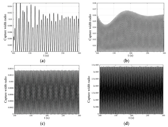
Figure 13.
Instantaneous capture width ratio with time for the MP–WEB with different frequency; , , , and . (a) ; (b) ; (c) ; and (d) .
Table 3.
The comparison between the capture width ratio results of the frequency domain and time domain.
5.3. Motion Response and Instantaneous Capture Width Ratio in Irregular Waves
Based on the former Equation (98), we could calculate the time domain motion response and capture width ratio of the MP–WEB in irregular waves. In order to avoid the influence factor, the size of the MP–WEB was the same as that of the above. The whole equipment had the same parameters as above, but the wave parameter could be set at different wave heights and spectrum peak periods according to the ISSC spectrum.
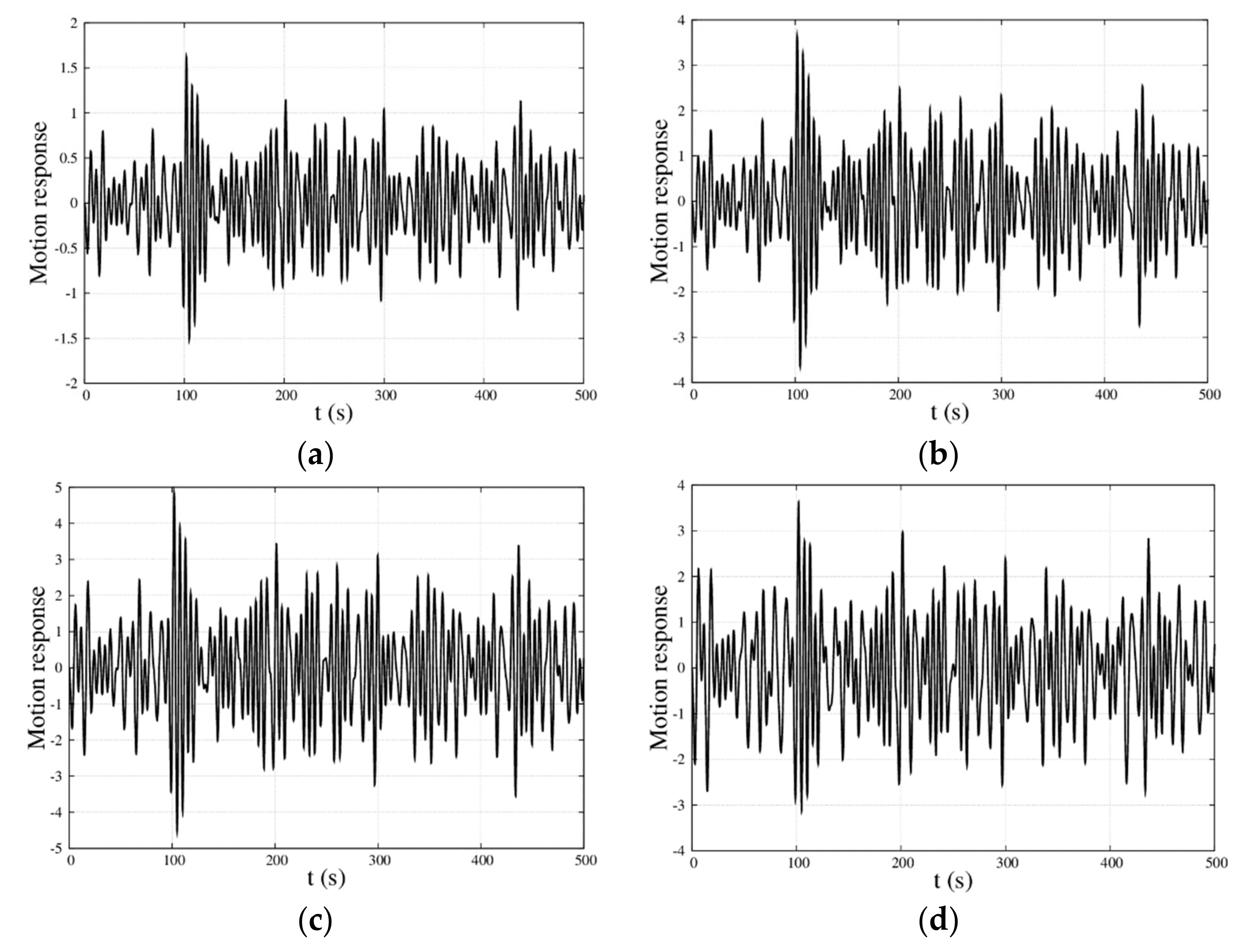
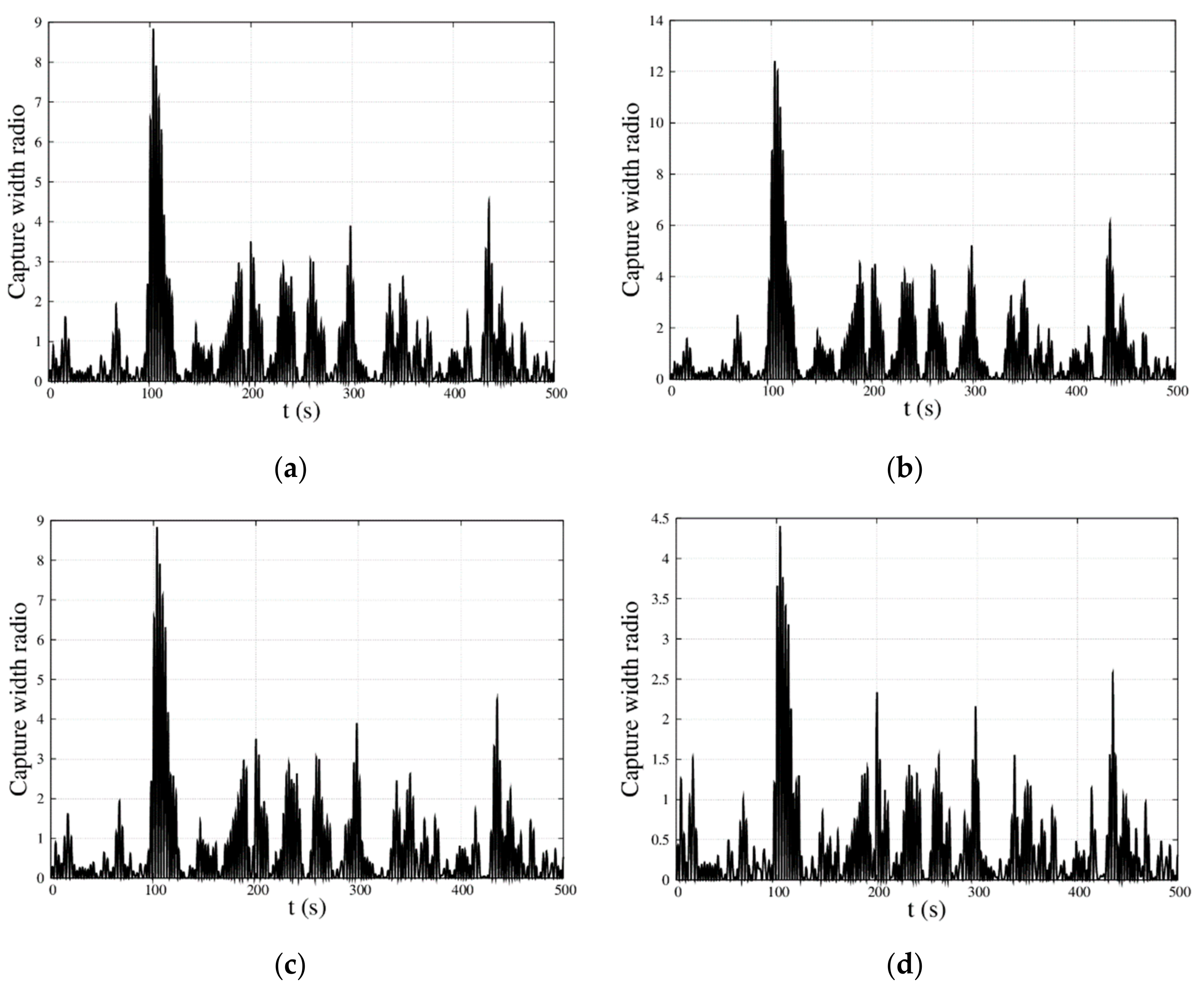
The motion response and capture width ratio of the MP–WEB in irregular waves with significant wave height and spectral peak period , respectively, are shown in Figure 14 and Figure 15. For the time domain motion response, it was obviously found that when the period was the same, the curve showed the same trend, but the amplitude values were different and increased with the significant wave height increase. For the capture width ratio, the best instantaneous capture width ratios were 8.837, 12.41, 8.837, and 4.405, respectively, and the average capture width ratios were 0.6116, 0.8558, 0.6116, and 0.3355, respectively for the different significant wave heights and spectral peak periods. Whatever the significant wave height was, the curves changed in exactly the same way as long as the spectral peak period was the same. In general, for the motion response, the significant wave height decided the amplitude value of the curves, and the spectral peak period decided the trend of the curves; for the capture width ratio, the change of curve only depended on the spectral peak period, and had nothing to do with the significant wave height.
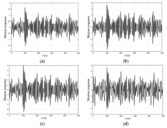
Figure 14.
Motion response with time for the MP–WEB in the irregular wave; . (a) ; (b) ; (c) ; and (d) .
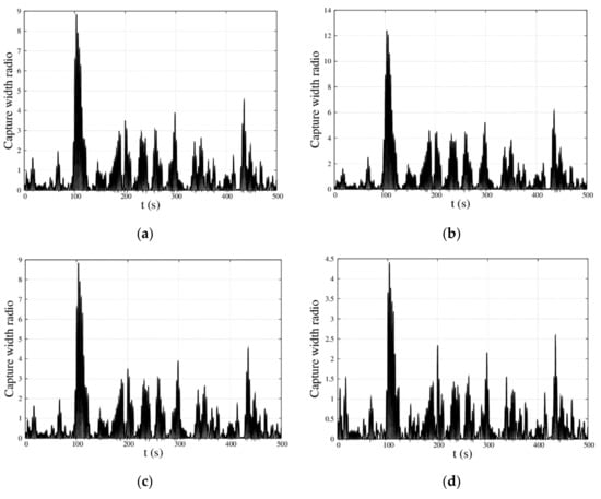
Figure 15.
Instantaneous capture width ratio with time for the MP–WEB in the irregular wave; . (a) ; (b) ; (c) ; and (d) .
6. Discussion
In this study, to improve the efficiency of converting energy from ocean waves, a new analytical solution was proposed to study a MP–WEB, allowing the user to design and optimize such devices according to different requirements. A number of case studies were performed by changing the main geometry parameters, and a code-to-code comparison verification was carried out. In particular, the influence of the PTO system characteristics on the system’s performance were parametrically investigated.
- (1)
- Based on the discussion of Reference [18], it could be seen from the comparison of axisymmetric buoy with and without the moonpool platform that the moonpool had an effect on the hydrodynamic coefficient of the central buoy. The hydrodynamic added mass and damping coefficients, as well as the wave force transfer functions, were substantially influenced by the geometry of the MP, and the identification of the trends allowed the derivation of the optimum dimensions according to the local environment conditions and energy requirements.
- (2)
- Compared with the motion characteristics of the buoy in Reference [18] and the moonpool in Reference [19], it could be seen that the wave gathering effect of the moonpool intensified the motion of the buoy, and the motion of the buoy promoted the motion of the moonpool. Considering the relative motion (RAO) between the buoy and the moonpool, it presented a strong dependence on the draft and radius of the MP. For different radius, the peak at radius at was about twice that at , but the peak frequencies showed little difference. Additionally, for different drafts, the peak at was about twice that at , and the peak frequencies differed by 0.9 (rad/s). In terms of the PTO damping coefficient, the maximum RAO at was 9% larger than that at . The capture width ratio at was 2.7 times larger than that at .
The difference between the time and frequency domain results was around 3%, demonstrating the correct implementation into the time domain model of the IRF method. When irregular waves were considered, the significant wave height had a moderate impact on the amplitude of the motion of the system, but the spectral peak period was the most important parameter, as it determined how close the energy in the spectrum was to the natural frequencies of the systems, and therefore, how much energy could be absorbed by the device from the waves.
Author Contributions
Conceptualization, F.K.; Methodology, D.Y. and F.J.; Software, J.A.; Validation, H.L. and H.C.; Writing—original draft preparation, W.S.; Writing—review and editing, H.L.; Funding acquisition, F.K.
Funding
This paper is financially supported by the National Natural Science Foundation (Grant No. 51979063, No. U1706227, No. 51779063 and No. 51679044), the High-tech Ship Research Projects Sponsored by MIIT-Floating Support Platform Project (the second stage) (MIIT201622), State Key Laboratory of Ocean Engineering (Shanghai Jiao Tong University) (Grant No. 1703) and the Fundamental Research Funds for the Central Universities (Grant No. HEUCFG201828 and No. HEUCFG201808).
Conflicts of Interest
The authors declare no conflict of interest. The funders had no role in the design of the study; in the collection, analyses, or interpretation of data; in the writing of the manuscript, or in the decision to publish the results.
References
- Ibrahim, Y.; Kamel, S.; Rashad, A.; Nasrat, L.; Jurado, F. Performance Enhancement of Wind Farms Using Tuned SSSC Based on Artificial Neural Network. Int. J. Interact. Multimedia Artif. Intell. 2019, 1, 1–7. [Google Scholar] [CrossRef]
- Elkasem, A.H.; Kamel, S.; Rashad, A.; Jurado, F. Optimal Performance of Doubly Fed Induction Generator Wind Farm Using Multi-Objective Genetic Algorithm. Int. J. Interact. Multimedia Artif. Intell. 2019, 5, 48–53. [Google Scholar] [CrossRef]
- Ulvgård, L. Wave Energy Converters: An Experimental Approach to Onshore Testing, Deployments and Offshore Monitoring. Acta Universitatis Upsaliensis, 21 September 2017. [Google Scholar]
- Hasanien, H.M. Gravitational search algorithm-based optimal control of archimedes wave swing-based wave energy conversion system supplying a DC microgrid under uncertain dynamics. IET Renew. Power Gener. 2016, 11, 763–770. [Google Scholar] [CrossRef]
- Penesis, I.; Manasseh, R.; Nader, J.R.; de Chowdhury, S.; Fleming, A.; Macfarlane, G.; Hasan, M.K. Performance of ocean wave-energy arrays in Australia. In Proceedings of the 3rd Asian Wave and Tidal Energy Conference (AWTEC 2016), Singapore, 24–28 October 2016; Volume 1, pp. 246–253. [Google Scholar]
- Franzitta, V.; Colucci, A.; Curto, D.; Curto, D.; di Dio, V.; Trapanese, M. A linear generator for a waveroller power device. In OCEANS 2017-Aberdeen; IEEE: Piscataway, NJ, USA, 2017; pp. 1–5. [Google Scholar]
- Mavrakos, S.A.; Katsaounis, G.M. Effects of floaters’ hydrodynamics on the performance of tightly moored wave energy converters. IET Renew. Power Gener. 2009, 4, 531–544. [Google Scholar] [CrossRef]
- Zang, Z.; Zhang, Q.; Qi, Y.; Fu, X. Hydrodynamic responses and efficiency analyses of a heaving-buoy wave energy converter with PTO damping in regular and irregular waves. Renew. Energy 2018, 116, 527–542. [Google Scholar] [CrossRef]
- Li, Y.; Yu, Y.H. A synthesis of numerical methods for modeling wave energy converter-point absorbers. Renew. Sustain. Energy Rev. 2012, 16, 4352–4364. [Google Scholar] [CrossRef]
- Falcão, A.F.O.; Henriques, J.C.C. Effect of non-ideal power take-off efficiency on performance of single- and two-body reactively controlled wave energy converters. J. Ocean Eng. Mar. Energy 2015, 1, 1–14. [Google Scholar] [CrossRef]
- Milani, F.; Moghaddam, R.K. Power Maximization of a Point Absorber Wave Energy Converter Using Improved Model Predictive Control. China Ocean Eng. 2017, 31, 510–516. [Google Scholar] [CrossRef]
- Bachynski, E.E.; Etemaddar, M.; Kvittem, M.I.; Luan, C.; Moan, T. Dynamic Analysis of Floating Wind Turbines during Pitch Actuator Fault, Grid Loss, and Shutdown. Energy Procedia 2013, 35, 210–222. [Google Scholar] [CrossRef]
- Yeung, R.W.; Peiffer, A.; Tom, N.; Matlak, T. Design, Analysis, and Evaluation of the UC-Berkeley Wave-Energy Extractor. J. Offshore Mech. Arct. Eng. 2012, 134, 46–51. [Google Scholar] [CrossRef]
- Liang, C.; Zuo, L. On the dynamics and design of a two-body wave energy converter. Renew. Energy 2017, 101, 265–274. [Google Scholar] [CrossRef]
- Dai, Y.; Chen, Y.; Xie, L. A study on a novel two-body floating wave energy converter. Ocean Eng. 2017, 130, 407–416. [Google Scholar] [CrossRef]
- Cho, I.H.; Kim, M.H. Hydrodynamic performance evaluation of a wave energy converter with two concentric vertical cylinders by analytic solutions and model tests. Ocean Eng. 2017, 130, 498–509. [Google Scholar] [CrossRef]
- Chen, X.B.; Liu, H.X.; Duan, W.Y. Semi-analytical solutions to wave diffraction of cylindrical structures with a moonpool with a restricted entrance. J. Eng. Math. 2015, 90, 51–66. [Google Scholar] [CrossRef]
- Liu, H.; Ao, J.; Chen, H.; Liu, M.; Collu, M.; Liu, J. Performance Analysis of a Sea Javelin Wave Energy Converter in Irregular Wave. J. Coast. Res. 2018, 83, 932–940. [Google Scholar] [CrossRef]
- Yoo, S.O.; Kim, H.J.; Lee, D.Y. Experimental and Numerical Study on the Flow Reduction in the Moonpool of Floating Offshore Structure. J. Offshore Mech. Arct. Eng.-Trans. ASME 2019, 141, 011301. [Google Scholar] [CrossRef]

© 2019 by the authors. Licensee MDPI, Basel, Switzerland. This article is an open access article distributed under the terms and conditions of the Creative Commons Attribution (CC BY) license (http://creativecommons.org/licenses/by/4.0/).