Optimising Convolutional Neural Networks to Predict the Hygrothermal Performance of Building Components


Abstract
1. Introduction
2. Optimising Convolutional Neural Networks (CNN)
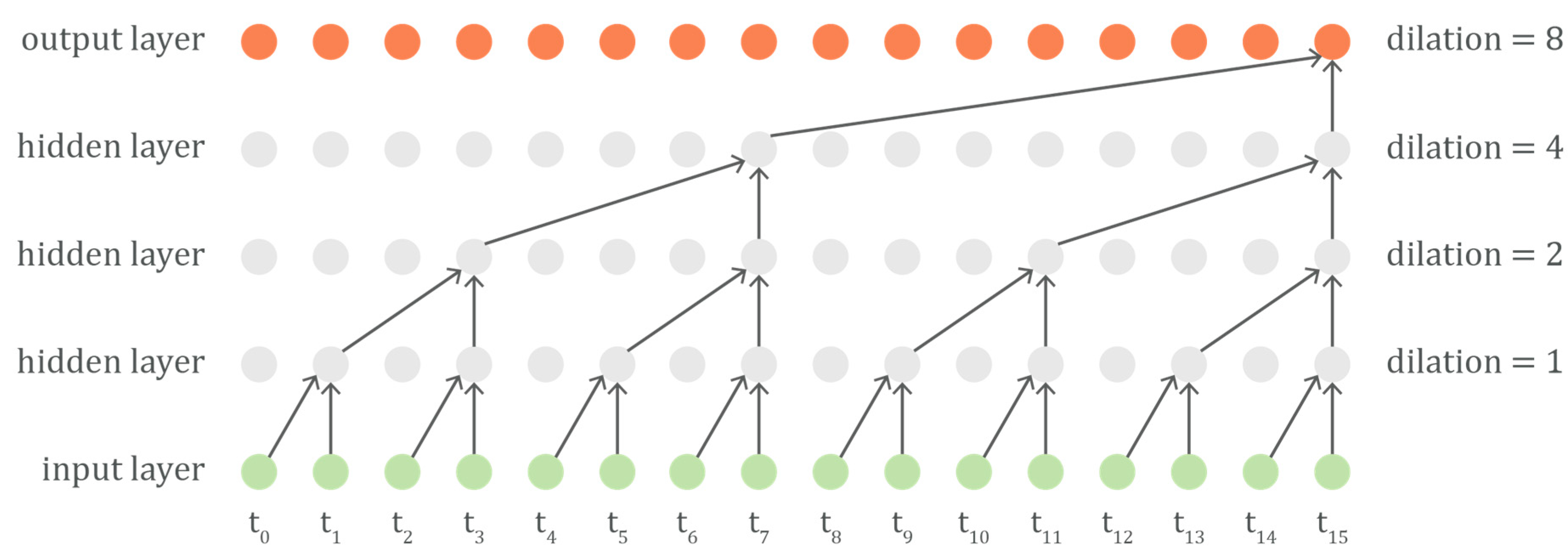
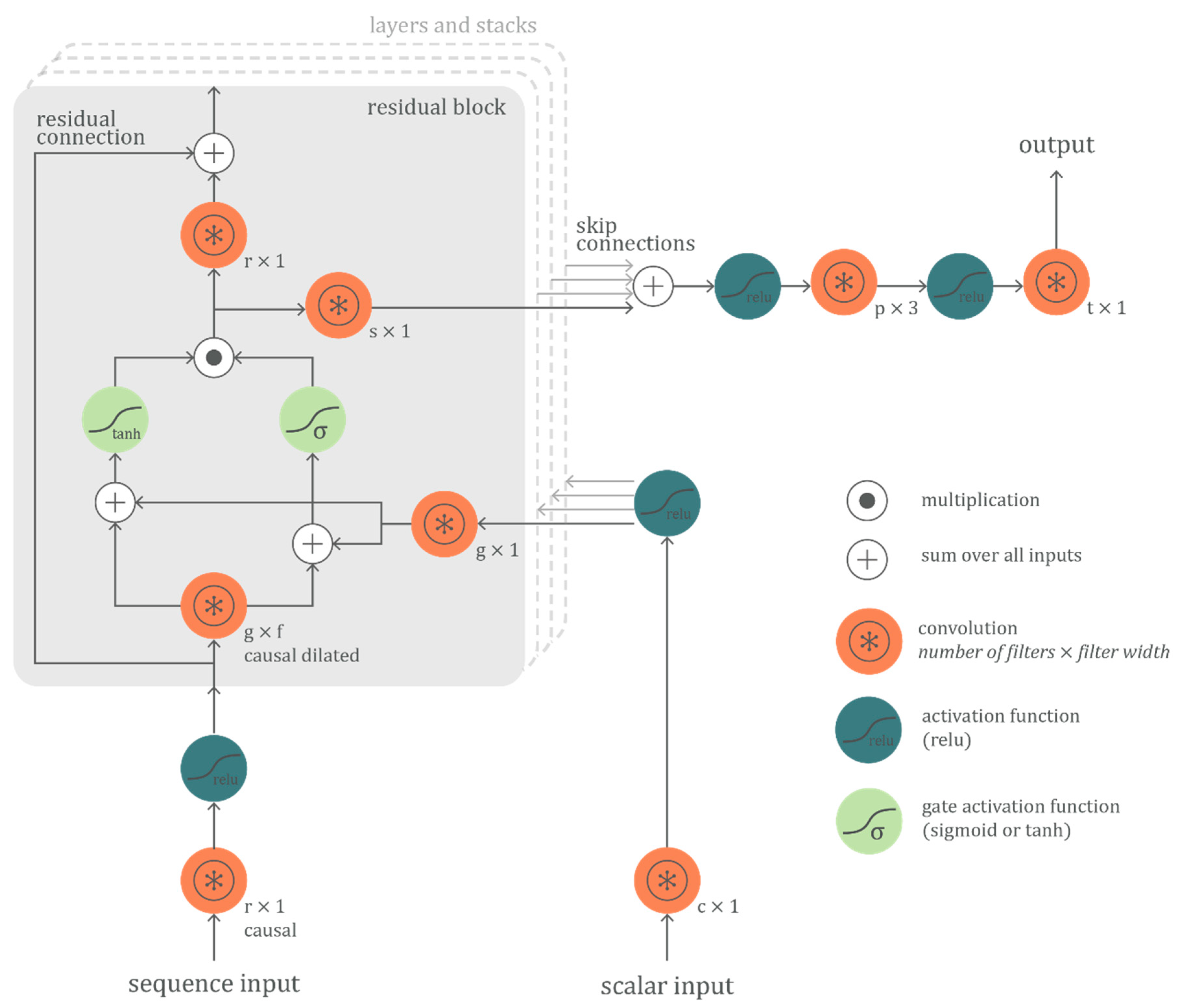
2.1. The Network Architecture
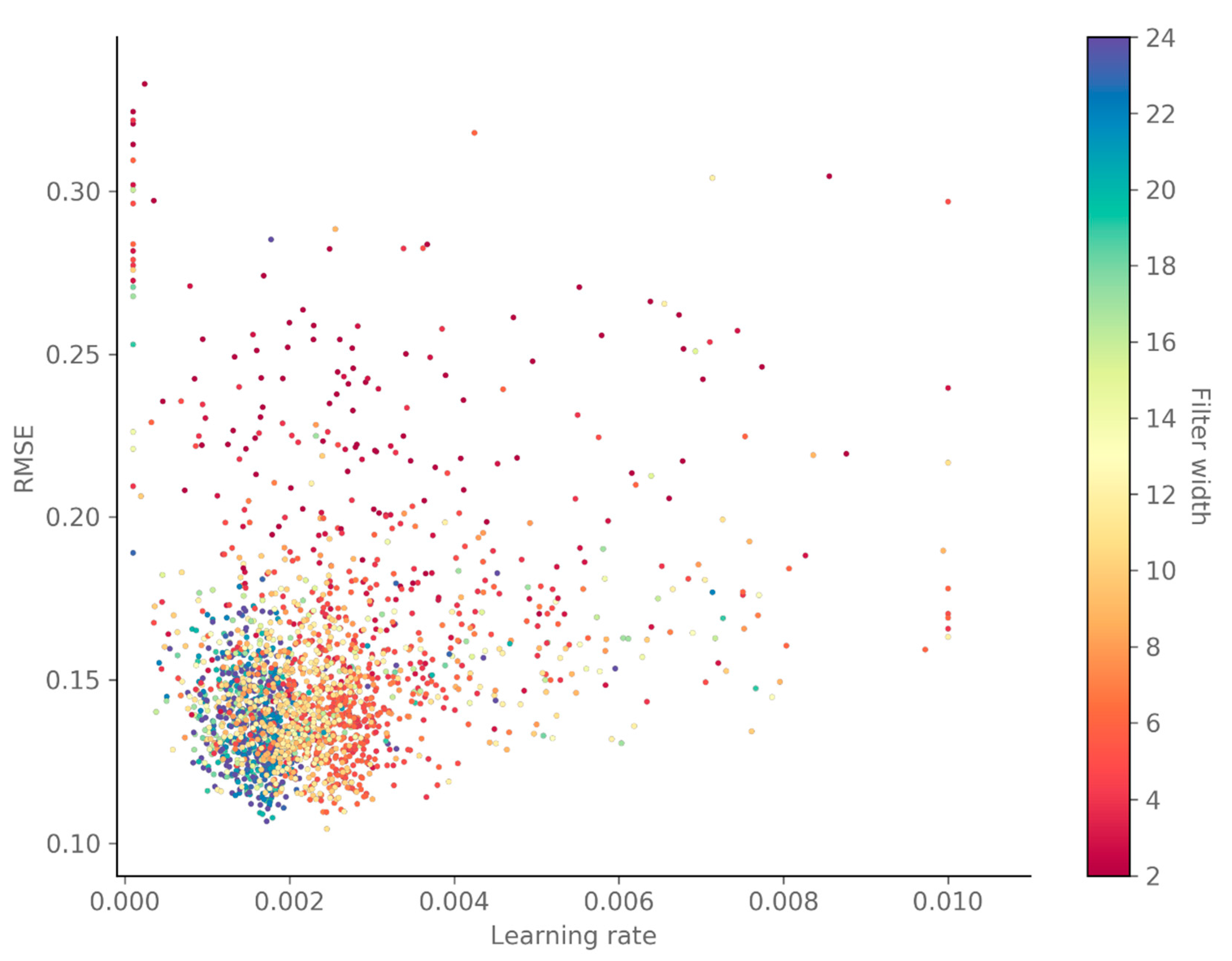
2.2. Hyper-Parameter Optimization
- Filter width f of causal dilated convolution
- Number of c-filters for initial conditional connection
- Number of g-filters for gate connections
- Number of s-filters for skip connections
- Number of r-filters for residual connections
- Number of p-filters for the penultimate connection
- Number of layers of residual blocks
- Number of stacks of layered residual blocks
- Loss function
- Learning algorithm
- Learning rate
- Number of training epochs
- Batch size
2.3. Performance Evaluation
3. Application
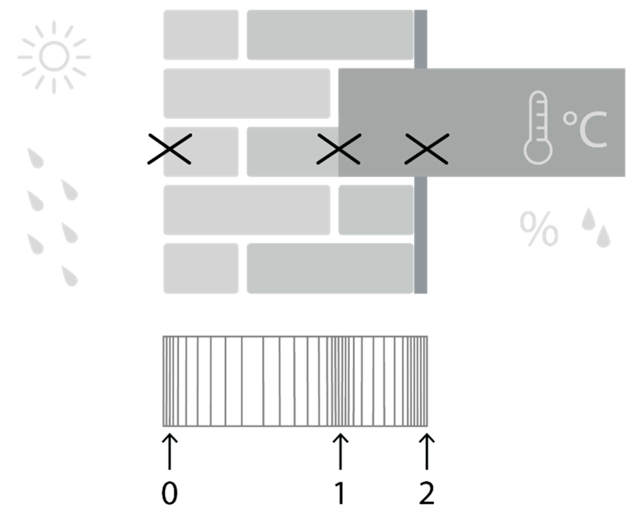
3.1. Hygrothermal Simulation Object
3.2. Training the Convolutional Neural Network
4. Results and Discussion
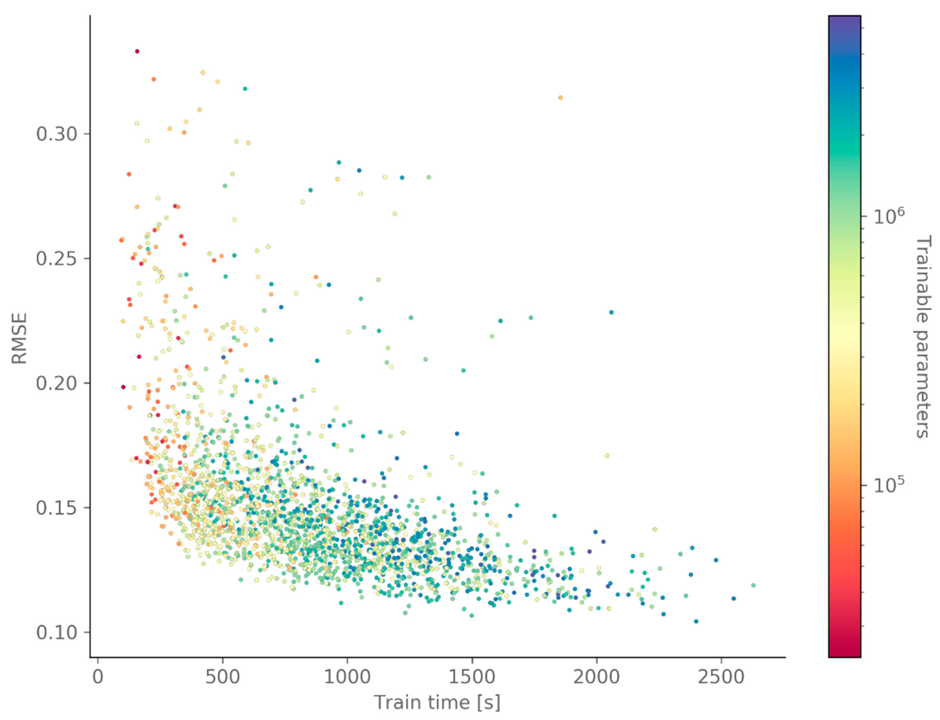
4.1. Hyper-Parameter Optimization
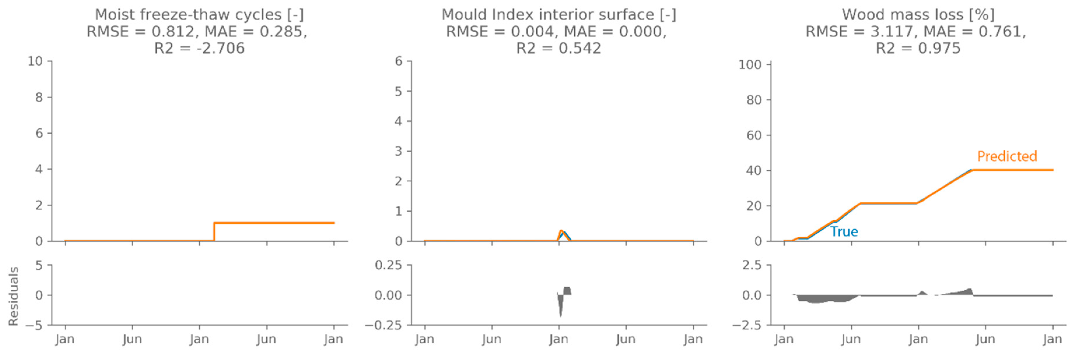
4.2. Performance Evaluation
5. Conclusions
Author Contributions
Funding
Conflicts of Interest
References
- Van Gelder, L.; Janssen, H.; Roels, S. Probabilistic design and analysis of building performances: Methodology and application example. Energy Build. 2014, 79, 202–211. [Google Scholar] [CrossRef]
- Janssen, H.; Roels, S.; Van Gelder, L. Annex 55 Reliability of Energy Efficient Building Retrofitting—Probability Assessment of Performance & Cost (RAP-RETRO). Energy Build. 2017, 155, 166–171. [Google Scholar]
- Vereecken, E.; Van Gelder, L.; Janssen, H.; Roels, S. Interior insulation for wall retrofitting—A probabilistic analysis of energy savings and hygrothermal risks. Energy Build. 2015, 89, 231–244. [Google Scholar] [CrossRef]
- Arumägi, E.; Pihlak, M.; Kalamees, T. Reliability of Interior Thermal Insulation as a Retrofit Measure in Historic Wooden Apartment Buildings in Cold Climate. Energy Procedia 2015, 78, 871–876. [Google Scholar] [CrossRef]
- Gradeci, K.; Labonnote, N.; Time, B.; Köhler, J. A proposed probabilistic-based design methodology for predicting mould occurrence in timber façades. In Proceedings of the World Conference on Timber Engineering, Vienna, Austria, 22–25 August 2016. [Google Scholar]
- Zhao, J.; Plagge, R.; Nicolai, A.; Grunewald, J. Stochastic study of hygrothermal performance of a wall assembly—The influence of material properties and boundary coefficients. HVACR Res. 2011, 9669, 37–41. [Google Scholar]
- Janssen, H. Monte-Carlo based uncertainty analysis: Sampling efficiency and sampling convergence. Reliab. Eng. Syst. Saf. 2013, 109, 123–132. [Google Scholar] [CrossRef]
- Van Gelder, L.; Janssen, H.; Roels, S. Metamodelling in robust low-energy dwelling design. In Proceedings of the 2nd Central European Symposium on Building Physics, Vienna, Austria, 9–11 September 2013; pp. 9–11. [Google Scholar]
- Gossard, D.; Lartigue, B.; Thellier, F. Multi-objective optimization of a building envelope for thermal performance using genetic algorithms and artificial neural network. Energy Build. 2013, 67, 253–260. [Google Scholar] [CrossRef]
- Bienvenido-huertas, D.; Moyano, J.; Rodríguez-jiménez, C.E.; Marín, D. Applying an arti fi cial neural network to assess thermal transmittance in walls by means of the thermometric method. Appl. Energy 2019, 233–234, 1–14. [Google Scholar] [CrossRef]
- Tijskens, A.; Roels, S.; Janssen, H. Neural networks for metamodelling the hygrothermal behaviour of building components. Build. Environ. 2019, 162, 106282. [Google Scholar] [CrossRef]
- Mirjalili, S.; Mirjalili, S.M.; Lewis, A. Grey Wolf Optimizer. Adv. Eng. Softw. 2014, 69, 46–61. [Google Scholar] [CrossRef]
- Vereecken, E.; Roels, S.; Janssen, H. Inverse hygric property determination based on dynamic measurements and swarm-intelligence optimisers. Build. Environ. 2018, 131, 184–196. [Google Scholar] [CrossRef]
- Borovykh, A.; Bohte, S.; Oosterlee, C.W. Conditional Time Series Forecasting with Convolutional Neural Networks. arXiv 2017, arXiv:1703.04691. [Google Scholar]
- Bai, S.; Kolter, J.Z.; Koltun, V. An Empirical Evaluation of Generic Convolutional and Recurrent Networks for Sequence Modeling. arXiv 2018, arXiv:1803.01271. [Google Scholar]
- van den Oord, A.; Dieleman, S.; Zen, H.; Simonyan, K.; Vinyals, O.; Graves, A.; Kalchbrenner, N.; Senior, A.; Kavukcuoglu, K. WaveNet: A Generative Model for Raw Audio. arXiv 2016, arXiv:1609.03499. [Google Scholar]
- Chollet, F. Keras. Available online: https://github.com/keras-team/keras (accessed on 15 May 2019).
- van den Oord, A.; Kalchbrenner, N.; Vinyals, O.; Espeholt, L.; Graves, A.; Kavukcuoglu, K. Conditional Image Generation with PixelCNN Decoders. In Proceedings of the Conference on Neural Information Processing Systems, Barcelona, Spain, 5–10 December 2016. [Google Scholar]
- He, K.; Zhang, X.; Ren, S.; Sun, J. Deep Residual Learning for Image Recognition. In Proceedings of the IEEE Conference on Computer Vision and Pattern Recognition (CVPR), Boston, MA, USA, 8–10 June 2015; Volume 19, pp. 107–117. [Google Scholar]
- Kingma, D.P.; Ba, J. Adam: A Method for Stochastic Optimization. arXiv 2014, arXiv:1412.6980. [Google Scholar]
- Vereecken, E.; Roels, S. Hygric performance of a massive masonry wall: How do the mortar joints influence the moisture flux? Constr. Build. Mater. 2013, 41, 697–707. [Google Scholar] [CrossRef]
- European Commission. Climate for Culture: Damage Risk Assessment, Economic Impact and Mitigation Strategies for Sustainable Preservation of Cultural Heritage in Times of Climate Change; European Commission: Brussels, Belgium, 2014. [Google Scholar]
- Blocken, B.; Carmeliet, J. Spatial and temporal distribution of driving rain on a low-rise building. Wind Struct. Int. J. 2002, 5, 441–462. [Google Scholar] [CrossRef]
- European Committee for Standardisation. EN 15026:2007—Hygrothermal Performance of Building Components and Building Elements—Assessment of Moisture Transfer by Numerical Simulation; European committee for Standardisation: Brussels, Belgium, 2007. [Google Scholar]
- Harrestrup, M.; Svendsen, S. Internal insulation applied in heritage multi-storey buildings with wooden beams embedded in solid masonry brick façades. Build. Environ. 2016, 99, 59–72. [Google Scholar] [CrossRef]
- Zhou, X.; Derome, D.; Carmeliet, J. Hygrothermal modeling and evaluation of freeze-thaw damage risk of masonry walls retrofitted with internal insulation. Build. Environ. 2017, 125, 285–298. [Google Scholar] [CrossRef]
- Marincioni, V.; Marra, G.; Altamirano-medina, H. Development of predictive models for the probabilistic moisture risk assessment of internal wall insulation. Build. Environ. 2018, 137, 257–267. [Google Scholar] [CrossRef]
- Delphin 5.8 [Computer Software]. Available online: www. http://bauklimatik-dresden.de/delphin (accessed on 15 May 2019).
- Viitanen, H.; Toratti, T.; Makkonen, L.; Peuhkuri, R.; Ojanen, T.; Ruokolainen, L.; Räisänen, J. Towards modelling of decay risk of wooden materials. Eur. J. Wood Wood Prod. 2010, 68, 303–313. [Google Scholar] [CrossRef]
- Vereecken, E.; Roels, S. Wooden beam ends in combination with interior insulation: An experimental study on the impact of convective moisture transport. Build. Environ. 2019, 148, 524–534. [Google Scholar] [CrossRef]
- Ojanen, T.; Viitanen, H.; Peuhkuri, R.; Lähdesmäki, K.; Vinha, J.; Salminen, K. Mold Growth Modeling of Building Structures Using Sensitivity Classes of Materials. In Proceedings of the Thermal Performance of the Exterior Envelopes of Buildings XI, Clearwater Beach, FL, USA, 5–9 December 2010; pp. 1–10. [Google Scholar]
- Hou, T.; Nuyens, D.; Roels, S.; Janssen, H. Quasi-Monte-Carlo-based probabilistic assessment of wall heat loss. Energy Procedia 2017, 132, 705–710. [Google Scholar] [CrossRef]


| Hyper-Parameter | Range |
|---|---|
| Number of filters | (25; 29) |
| Number of filters | (25; 29) |
| Number of filters | (25; 29) |
| Number of filters | (25; 29) |
| Number of filters | (25; 29) |
| Filter width | (2; 24) |
| Number of layers | (1; 8) |
| Number of stacks | (1; 4) |
| Learning rate | (0.0001; 0.01) |
| Parameter | Value |
|---|---|
| Exterior climate | D (Gent; Gaasbeek; Oostende, St Hubert) |
| Exterior climate start year | D (2020; 2047) |
| Wall orientation (degrees from North) | U (0; 360) |
| Solar absorption (-) | U (0.4; 0.8) |
| Ext. heat transfer coefficient slope (J/m3K) | U (1; 8) |
| WDR exposure factor (-) | U (0; 2) |
| Brick wall thickness (m) | U (0.2; 0.5) |
| Brick material | D (Brick 1; Brick 2; Brick 3) |
| Interior humidity load [24] | D (load A; load B) |
| Parameter | Brick 1 | Brick 2 | Brick 3 |
|---|---|---|---|
| Dry thermal conductivity (W/m2K) | 0.87 | 0.52 | 1.00 |
| Dry vapour resistance factor (-) | 139.52 | 13.25 | 19.00 |
| Capillary absorption coefficient (kg/m2s0.5) | 0.046 | 0.357 | 0.100 |
| Capillary moisture content (m3/m3) | 0.128 | 0.266 | 0.150 |
| Saturation moisture content (m3/m3) | 0.240 | 0.367 | 0.250 |
| Parameter | Value |
|---|---|
| Exterior surface | |
| Long wave emissivity | 0.9 |
| Interior surface | |
| Total heat transfer coefficient h (W/m2K) | 8 |
| Moisture transfer coefficient β (s/m) | 3 × 10⁻⁸ |
| Initial conditions | |
| Initial temperature (°C) | 20 |
| Initial relative humidity (%) | 50 |
| Damage Pattern | Prediction Model | Required Hygrothermal Time Series |
|---|---|---|
| Frost damage | Moist freeze-thaw cycles | T, RH, saturation degree |
| Decay of wooden beam ends | VTT wood decay model | T, RH |
| Mould growth | Updated VTT mould growth model | T, RH |
| Conditional Filters | Gate Filters | Skip Filters | Residual Filters | Penultimate Filters | Filter Width | Layers | Stacks | Learning Rate | |
|---|---|---|---|---|---|---|---|---|---|
| 1 | 256 | 512 | 256 | 128 | 64 | 11 | 3 | 3 | 0.00245 |
| 2 | 256 | 256 | 256 | 512 | 64 | 24 | 3 | 2 | 0.00172 |
| 3 | 256 | 512 | 256 | 128 | 128 | 11 | 3 | 3 | 0.00220 |
| 4 | 256 | 256 | 256 | 256 | 128 | 20 | 3 | 2 | 0.00179 |
| 5 | 128 | 512 | 512 | 256 | 128 | 20 | 3 | 2 | 0.00167 |
| 6 | 32 | 512 | 256 | 256 | 64 | 20 | 3 | 2 | 0.00164 |
| 7 | 128 | 64 | 128 | 256 | 256 | 6 | 5 | 3 | 0.00245 |
| 8 | 128 | 64 | 128 | 256 | 256 | 7 | 5 | 3 | 0.00241 |
| 9 | 128 | 512 | 128 | 64 | 128 | 12 | 3 | 3 | 0.00266 |
| 10 | 128 | 128 | 128 | 128 | 128 | 6 | 6 | 3 | 0.00263 |
© 2019 by the authors. Licensee MDPI, Basel, Switzerland. This article is an open access article distributed under the terms and conditions of the Creative Commons Attribution (CC BY) license (http://creativecommons.org/licenses/by/4.0/).
Share and Cite
Tijskens, A.; Janssen, H.; Roels, S. Optimising Convolutional Neural Networks to Predict the Hygrothermal Performance of Building Components. Energies 2019, 12, 3966. https://doi.org/10.3390/en12203966
Tijskens A, Janssen H, Roels S. Optimising Convolutional Neural Networks to Predict the Hygrothermal Performance of Building Components. Energies. 2019; 12(20):3966. https://doi.org/10.3390/en12203966
Chicago/Turabian StyleTijskens, Astrid, Hans Janssen, and Staf Roels. 2019. "Optimising Convolutional Neural Networks to Predict the Hygrothermal Performance of Building Components" Energies 12, no. 20: 3966. https://doi.org/10.3390/en12203966
APA StyleTijskens, A., Janssen, H., & Roels, S. (2019). Optimising Convolutional Neural Networks to Predict the Hygrothermal Performance of Building Components. Energies, 12(20), 3966. https://doi.org/10.3390/en12203966