An Integration Optimization Method for Power Collection Systems of Offshore Wind Farms

Abstract

The traditional power collection system design separately optimizes the connection topology and the cable cross sections, which may result in the inherent shortcoming of lacking the most economical solutions. In this pursuit, the present work envisages the development of an integrated design method for general wind farm power collection systems, which integrated the coupling random fork tree coding, union-find set loop identification, current and voltage drop calculation models, and a high performance optimization algorithm. The proposed coupling random fork tree coding, for the first time, realized the coupling code of the substation location, connection topology, and cable cross sections, providing the basis for the integration design of the power collection system. The optimization results for discrete and regular wind farms indicated that the proposed integration method achieved the best match of topology, substation location, and the cable cross sections, thus presenting the most economical scheme of the power collection system. Compared to the traditional two-step methods, the integration method used more branches while acquiring them, to maintain the lower number of wind turbines in each branch. Furthermore, it also employed large cross-section cables to reduce the energy loss caused by the impedance in the topology, thereby resulting in a slight increased cable cost; however, the total cost was minimized. The proposed method is very versatile and suitable for the optimization of power collection systems containing any number of wind turbines and substations, and can be combined with any evolutionary algorithm.

1. Introduction

The global focus on wind farm development has shifted from land to ocean. Compared to land, offshore wind energy resources have many advantages, including richer reserves, higher wind energy density, smaller turbulence intensity, and more stable wind direction, which have great development potential [1]. At present, the development cost of the offshore wind farms is more than twice that of the onshore wind farms, and the expenditure for the power collection systems accounts for 15%–30% of the total investment of the project [2]. Therefore, the current research focuses on establishing more cost-effective power collection systems.

The optimization of the offshore wind farm power collection system consists of three aspects, viz. the connection topology, the number and locations of substations, and the planning of the cable cross sections. Only an integration optimization combining these three aspects can unanimously obtain the most economical solution [3,4]; however, subject to the lack of integrated design methods, the current design of these three aspects is carried out separately according to their respective guidelines and constraints.

The optimization of the connection topology is inspired by graph theory in computer science, wherein the wind turbine and the connection topology are regarded as nodes and directed connected graphs, respectively. Therefore, the related methods in graph theory were introduced to obtain the topology with the shortest total length. Among them, the minimum spanning tree (MST) is the most widely used model [5,6,7,8,9,10,11]. In this regard, the first attempt was made by Vasko et al., by a transformation of the connection topology of the wind farm into the minimum spanning tree and shortest path problem, and development of a neighbourhood search step. In the literature [6], the clustering algorithm was introduced into the connection topology optimization using the following steps: Firstly, the wind turbine groups were clustered using the genetic algorithm, and then the wind turbines in each group were used to generate the connection network. In addition, other more efficient clustering algorithms were also applied in the optimization of the topology, such as k-mean clustering [7] and fuzzy c-means clustering [8]. Under the MST architecture, the constraint values were evaluated after the topology was obtained. The resulting topology faced a difficulty to satisfy all constraints at once, which required a prior adjustment, based on experience. For example, the capitalized MST and the dynamic MST were employed separately to enhance the processing power of a large number of constraints in the optimization of the topology [9,10]. Another applied graph-based model employed in the literature is the travelling salesman problem model [12,13], which obtained the optimal topology by traversing all nodes to form a collection containing multiple different shortest paths. In addition, a hop-indexed integer programming formulation to achieve the optimization of the string topology was introduced by Bauer et al. [14], which replaced the graph theory method, by constructing a connection matrix combined with a random algorithm. Furthermore, Rodrigues et al. [15] developed a multi-objective optimization method framework for network topologies and corresponding electrical facilities that took into account a large number of engineering details.

The number and location of substations have a significant impact on the connection topology, and several studies aimed to obtain the optimal match between these two factors [16,17,18,19,20,21,22,23,24]. In these studies, the shortest cable length [17,18], minimal investment [15], highest gain [19], and a minimal energy loss [20] were the optimization objectives, and the substation’s spatial coordinates were used as variables. These were combined with the optimization algorithm to obtain the best substation location and the corresponding matching topology structure. Very few studies have been done to improve the economics of the entire wind farm by jointly optimizing the wind farm fleet location and the connection topology for a given annual wind speed distribution [21,22,23]. In the selection of the optimized algorithm, the optimization of the power collection system involves complex connections between the wind turbines and the substations, and a large number of constraints on power parameters exist, like being revealed as a non-convex, discontinuous, and NP-complete complex optimization [3]. In order to cope with such problems, evolutionary algorithms such as genetic algorithms [17,18] and Particle Swarm Optimization algorithm [21] are considered to be ideal optimization algorithms, since they can be applied to any number of design variables and can tolerate random errors generated during the search process. In addition, classical optimization algorithms such as nonlinear programming [20,24] and quadratic programming [25] have also been applied.

The cable cross-section planning usually involves assigning a suitable cross-section cable to each connection based on the principle that the maximum current does not exceed the allowable current carrying capacity of the cable after obtaining an optimized topology [8,26]. At the same time, safety and economic constraints, such as line voltage drop [27] and thermal stability [28], also needs to be strictly met.

From the literature review, the optimization of the current wind farm power collection system is usually a two-step method [29]: First, optimizing the connection topology under the condition of a fixed or variable substation location, and secondly, planning the cross section of each cable segment. There are two obvious shortcomings in this two-step approach:

(1)

In the two-step method, the essence of the optimization of the connection topology is to obtain the topology with the shortest total cable length. However, when a cable with a different cross section is assigned to each segment of the topology, due to the cable’s current-carrying constraint, the superimposing additional weights may lead to a result that the proposed topology is not the most economical one [29].

(2)

After the cable cross section is allocated according to the current-carrying capacity, the solution is obtained with the smallest cross section of each cable segment in the topology, which minimizes the cable cost. However, the smaller the cross section of the cable, the greater is the resistance. This results in a greater power loss in the service life of the power system by 20 to 30 years. It is reported that by using a large-section cable properly on a large-flow cable section, the power loss caused by the resistance can be greatly reduced, thereby effectively improving the economic efficiency of the system [30].

In order to overcome the above shortcomings, initially we developed an integration optimization method to achieve the best matching of topology and cable cross sections, which involved the proposed integrated coding scheme, power parameter calculation model, and high-performance evolution algorithm. Subsequently, the characteristics and performance of the method were illustrated by optimizing the power collection system of a discrete wind farm.

2. Mathematical Modelling

2.1. Proposed Coding Scheme

The traditional two-step method adopts the design idea of optimizing the connection topology first, then redistributing the cross section of the cable, and may not get the most economical solution. In order to realize the integration optimization of the connection topology and the cable cross section allocation, a new connection topology coding scheme was proposed, which is called coupled random fork tree coding (CRFTC). CRFTC is a combination of three parts of the variable, as shown in Equation (1).

$$\mathit{X}={\mathit{X}}_{\mathit{I}}\cup {\mathit{X}}_{\mathit{I}\mathit{I}}\cup {\mathit{X}}_{\mathit{I}\mathit{I}\mathit{I}},$$

(1)

where

$$\begin{array}{l}{\mathit{X}}_{\mathit{I}}=\{x_{S,1},\dots ,x_{S,N_{os}},y_{S,1},\dots ,y_{S,N_{os}}\}\\ {\mathit{X}}_{\mathit{I}\mathit{I}}=\{x_1,x_2,\dots ,x_j,\dots ,x_{N_{WT}}\}\\ {\mathit{X}}_{\mathit{I}\mathit{I}\mathit{I}}=\{x_{C,1},x_{C,2},\dots ,x_{C,k},\dots ,x_{C,N_C}\}\end{array}.$$

In this case, N_OS and N_WT are the number of substations and wind turbines in the wind farm, respectively.

The first part variable X_I represents the spatial coordinates of the substations. The coordinates of any substation i are real variables, expressed as (x_s,i, y_s,i), so the number of variables in this part is twice the number of substations. The second part variable X_II represents the connection between wind turbines and substations; the variable x_j represents the number of the wind turbine or substation to which the wind turbine j current flows, which is an integer variable. The final part variable X_III represents the type of each cable cross section; the variable x_C,j represents the cable type of cable segment k, which is an integer variable. A total of (2N_OS + N_WT + N_C) variables were set for the entire scheme, and each variable was randomly generated.

It can be seen that, in the above-mentioned random generation topology of the coding scheme, any one wind turbine was connected to only one other wind turbine or substation, but also could be connected by a plurality of other wind turbines. At the same time, if there was no loop in the topology, a connection was made from each wind turbine, which inevitably formed a standard tree topology.

Our proposed coding scheme completely describes the wind farm power network topology in a simple way, is very easy to program, and can be combined with any evolutionary algorithm.

2.2. Loop Identification Model

The existence of a loop is not allowed in a tree topology. In this study, first, the loops in the topology were identified and counted, and then the constraint processing mechanism was used to exclude the loops in the topology during the evolution process.

The loop recognition adopts the union-find set algorithm of the graph theory [31]. The basic idea is constructing a subset S_i of any wind turbine WT_i in the network, which is initially empty, and, taking V_i as the starting point and leading to the substation, there must be a connecting branch containing n edges Es = { E_s,1,…,E_s,i,…,E_s,n}.

First, starting from WT_i, point along the cable E_i to the endpoint WT_i+1, and retrieve whether WT_i and WT_i+1 have existed in S_i at the same time. If it exists, it indicates that there is a loop and the search stops. If not, WT_i and WT_i+1 are stored in the subset S_i while WT_i+1 is taken as a new starting point, and the end point WT_i+2 is found along the cable segment E_i+1, again judging whether WT_i+1 and WT_i+2 have existed simultaneously in S_i. The above steps are repeated until the end point judgment of all sides in the branch Es are completed.

Repeating the above process for all wind turbines in the network gave all the loop counts in the network from Equation (2).

$$N_{Loop}=\{\begin{array}{ll}{N}_{Loop}+1,& (W{T}_i\in {\mathit{S}}_i)\wedge (W{T}_{i+1}\in {\mathit{S}}_i),i=1,2,\mathrm{∆},n-1\\ N_{Loop},& otherwise\end{array},$$

(2)

where N_Loop is the total number of loops in the topology, which is initially 0.

2.3. Cost Model

We systematically carried out the optimization research at a tree-topological offshore wind farm power collection system. The total cost C_Total given by Equation (3) considered the investment cost of the medium-voltage submarine cable and the energy loss cost in the operation of the power system, superposed by three parts: The medium voltage cable cost C_Cable, the construction cost C_Construction, and the energy loss cost C_Loss:

$$C_{Total}=C_{Cable}+C_{Construction}+C_{Loss}.$$

(3)

The medium voltage cable cost C_Cable is a function of the length and cross-sectional area of the cable and can be obtained from by Equation (4):

$$C_{Cable}={\displaystyle \sum _{i=1}^{N_C}3\cdot L_{i,j}^M\cdot c_j^M},j\in N_{CS},$$

(4)

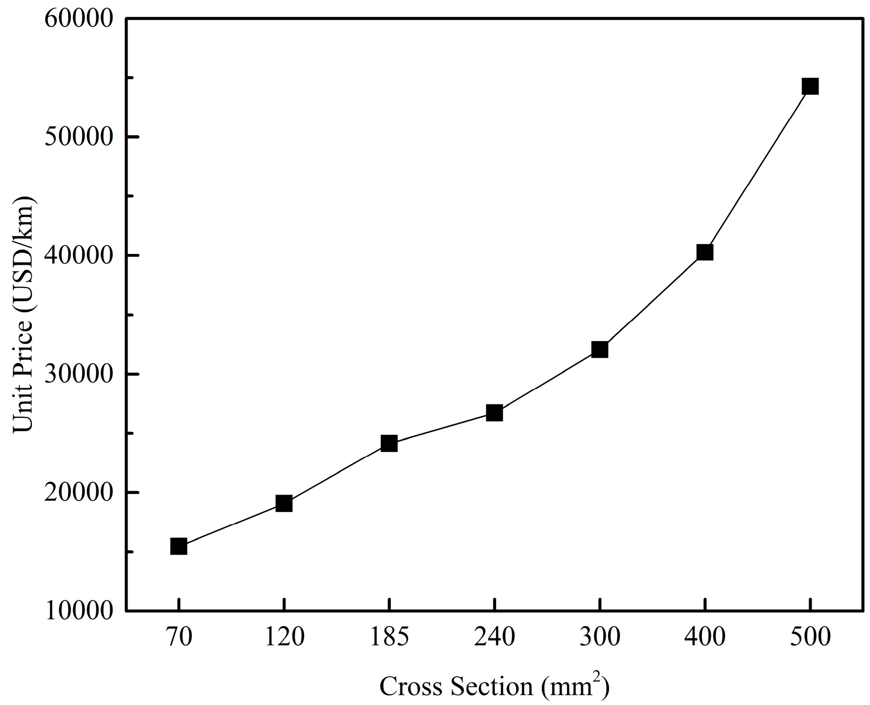
where N_C is the number of medium voltage cable segments; $L_{i,j}^M$ and $c_j^M$ are the length of the i-th medium voltage cable section and the corresponding unit length cable price; and N_CS is the number of cable types. In this study, the medium voltage power network was built using 30 kV, and the choice of cables covered seven cross-sections from 70 mm² to 500 mm². As shown in Figure 1 and Figure 2, the cost and basic technical parameters of the cable were obtained from earlier work [30]. The price of the cable is quoted in the reference in Euro, which is converted to United States Dollar (USD) denominated at a rate of 1 Euro = 1.107 USD.

The construction cost C_Construction is the cost of trench mining for submarine cables, and is given by Equation (5):

$$C_{Trench}={\displaystyle \sum _{i=1}^{N_C}{L}_{i,j}^M}\cdot c_T,$$

(5)

where c_T is the construction cost per unit length, which is 21,000 USD/km according to engineering experience [29].

The energy loss cost C_Loss is the sum of the energy loss costs of the power network topology lifetime, and is given by Equation (6):

$$C_{Loss}={\displaystyle \sum _{i=0}^{\tau -1}{\left(1+q\right)}^i{E}_{AL}}{c}_{EP},$$

(6)

where τ is the design life of the wind farm power system, defined as 20 years; q is the discount factor, defined as 0.02; E_AL is the annual power loss of the power network, and c_EP is the unit price of the wind farm sold to the grid, defined as 50 USD/MWh [32].

2.4. Annual Energy Loss Model

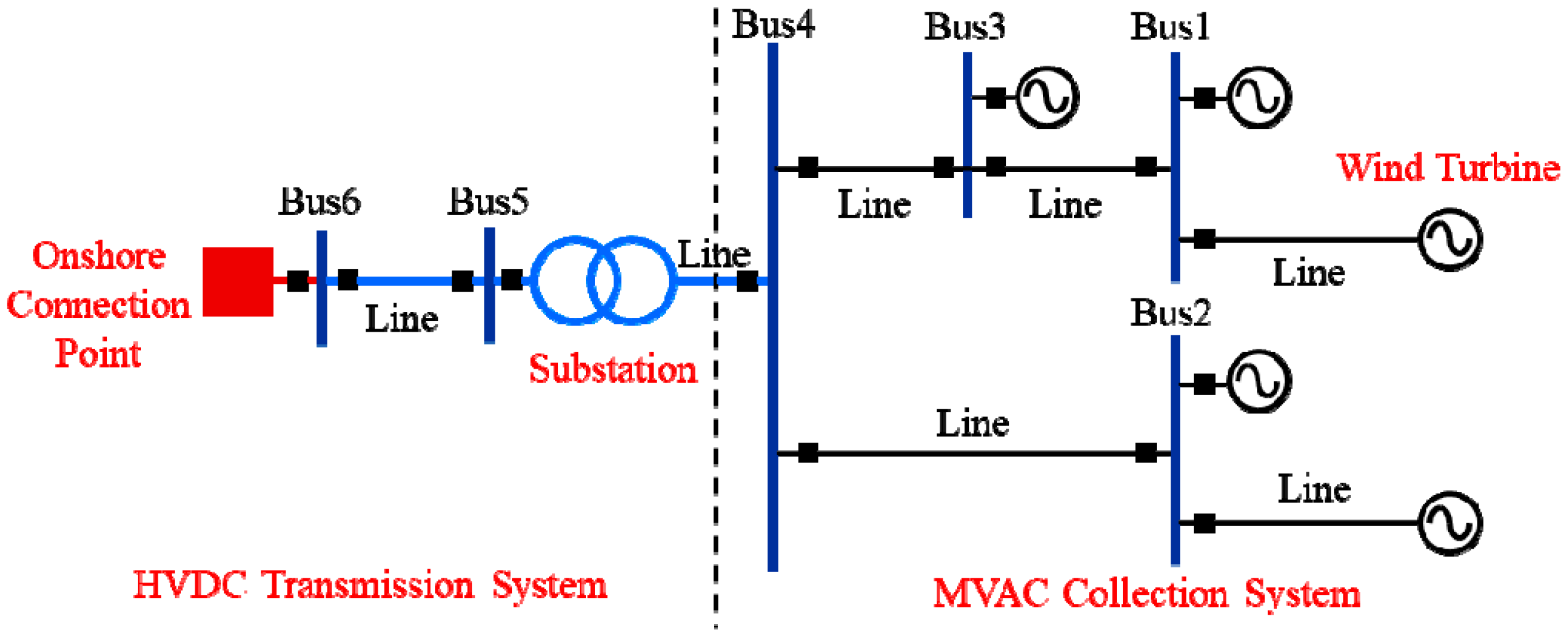
The calculation of the annual energy loss of the wind farm power collection system is complex, and it is necessary to analyse the energy loss in all cable segments under a specific annual wind speed distribution. A typical tree power system architecture with five wind turbines is shown in Figure 3. The expression for the calculation of annual energy loss is given by Equation (7):

$$E_{AL}={\displaystyle {\int }_{V=3}^{25}\left({\displaystyle \sum _{i=1}^{N_C}\left(I_i^2(V)R_i\right)}\right)f(V)TdV},$$

(7)

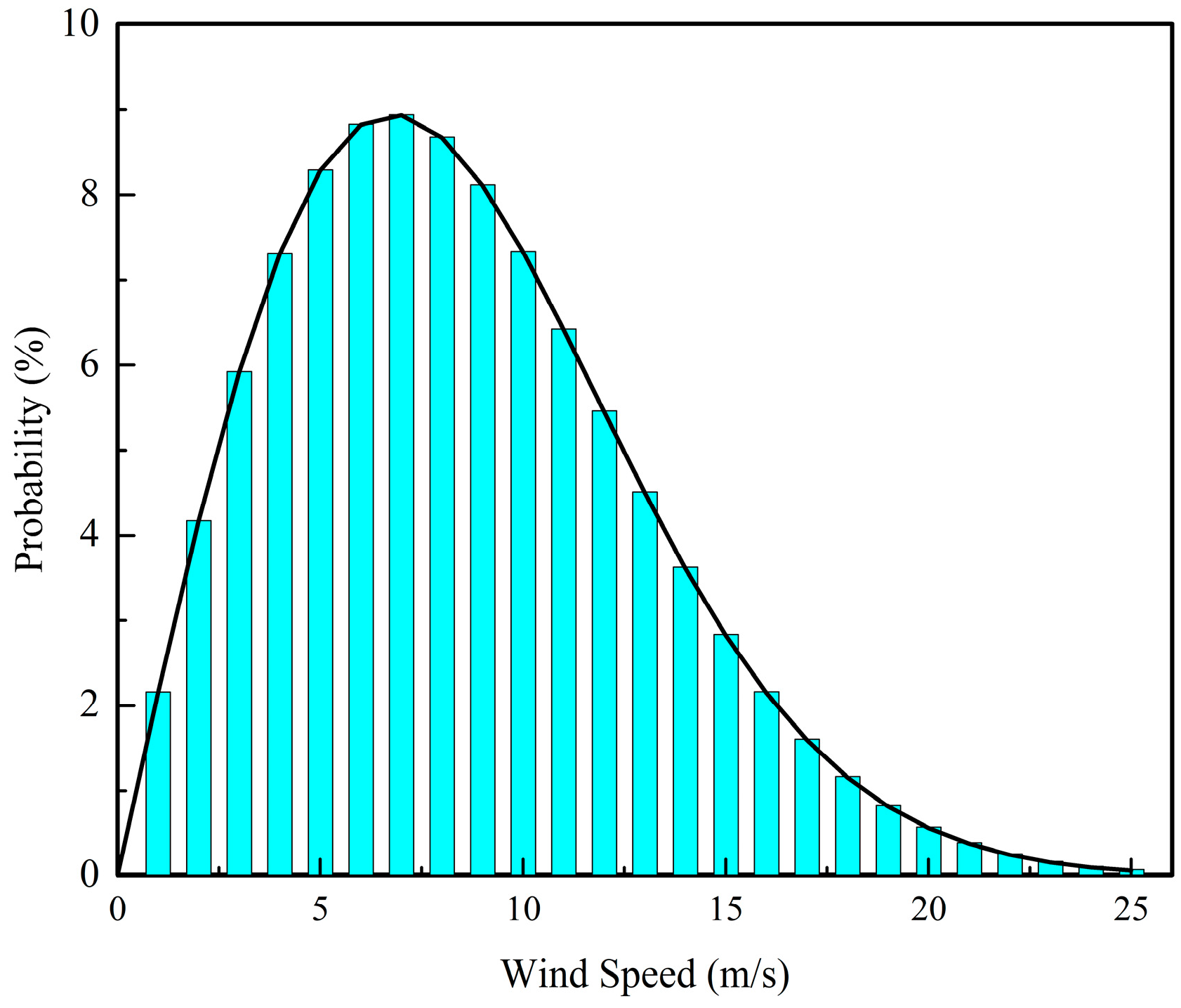
where V is the wind speed of the wind field; I_i (V) is the current on cable segment i when the wind speed is V; T is the number of hours per year; and f () is the Weibull probability distribution function. As shown in Figure 4, the assumptions are based on the Class II wind farm setting of the GL2010 design standard. The Weibull shape parameter and the annual mean wind speed distribution were 2 and 8.5 m/s, respectively.

The rated current of the cable segment needs to be included in the sum of the currents generated by all the wind turbines flowing through it to the substation. To calculate the rated current of any cable segment i, a subset of the cable segment SV_i is needed to store the number of the wind turbine group. The current at the wind speed V of the cable segment I can be calculated by Equation (8) as follows:

$$I_i(V)={\displaystyle \sum _{j=1}^{N_{F,i}}\left(\frac{P_j(V)/\cos \phi }{\sqrt{3}{U}_N}\right)},\hspace{1em}\forall j\in \mathit{S}{\mathit{V}}_i,$$

(8)

where P_j (V) is the output power of wind turbine j at wind speed V; U_N is the rated voltage of the medium voltage network; and $\cos \phi$ is the power factor.

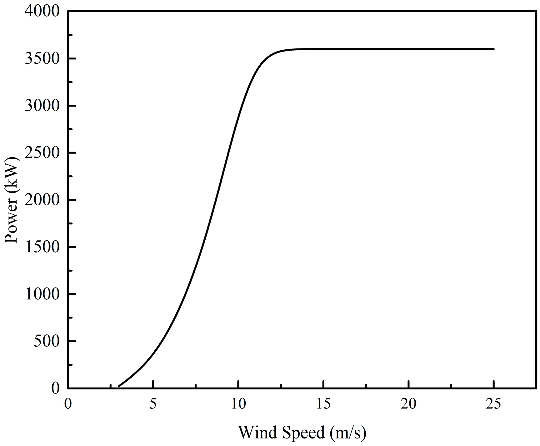
In this study, the Siemens 3.6 MW wind turbine is selected to form the offshore wind farms as the energy input to the power networks. The power curve power as a function of wind speed is shown in Figure 5. The power loss caused by the wake effect between wind turbines was ignored.

The real-time output of a wind turbine varies significantly with the wind speed, resulting in a dramatic change in the current passing through the conductor. In order to evaluate the energy loss more accurately, it is necessary to consider the influence of load variation on conductor resistance. The cable resistance R(T) per unit length at the temperature T is calculated by the following equation:

$$R(T)=R_0\left[1+a_{20}(T-T_0)\right],$$

(9)

where R₀ is the conductor resistance at 20 °C (Ω/m), which is provided as standard data by the manufacturers; a₂₀ is the constant mass temperature coefficient (a₂₀ = 0.00403 °C⁻¹ for aluminium); and T₀ is the reference ground temperature.

Conductor temperature is determined by load and can be approximately evaluated based on the following empirical equation, which derives from the equations of the conductor thermodynamic balance in a homogenous environment:

$$R(T)=T_0+{\left(\frac{I}{I_{pc}}\right)}^2\left(T_{\max }-T_0\right),$$

(10)

where T_max is the maximum permissible conductor temperature; and I and I_pc are the load current and maximum permissible continuous current of the cable, respectively.

2.5. Branch Voltage Drop Model

The maximum voltage drop in each branch in the topology must be controlled within a certain range. After each cable segment was determined to have a cross section, its impedance, maximum current carrying capacity, etc., were determined. A subset SF_i was created for each branch F_i to hold the number of all cable segments subordinate to this branch, and then the maximum voltage drop $\mathsf{\Delta }{U}_{F,i}$ for this branch was calculated using the formula in Equation (11) [29,30].

$$\mathsf{\Delta }{U}_{F,i}={\displaystyle \sum _{j=1}^{N_{F,i}}\sqrt{3}{L}_j{I}_{E,j}}\left(R_j\cos {\varphi }_j+X_j\sin {\varphi }_j\right)\hspace{1em}\forall j\in \mathit{S}{\mathit{F}}_i,$$

(11)

where N_F,i is the number of cable segments in SF_i; R_j and X_j are the conductor resistance and inductive reactance of the cable segment j, respectively; L_j is the length of the cable segment j; I_E,j is the rated current of the cable segment j as all wind turbines in the branch reach the rated power; and $\cos {\varphi }_j$ is the power factor of the the cable segment j.

3. Description of the Optimization Problem

The minimum total cost of the power network was optimized, and a large number of equations and inequality constraints were met, which included (1) the current of any cable segment was less than the allowable current carrying capacity of the cable, (2) the voltage drop across each branch was less than the allowable voltage drop, and (3) the number of loops across the network was zero.

$$\min \hspace{1em} C_{Total}(\mathit{X}).$$

(12)

It satisfies:

$$\{\begin{array}{ll}{I}_i<I_{P,i},& \forall i=1,2,\dots ,N_C\\ \mathsf{\Delta }{U}_{F,j}<\mathsf{\Delta }{U}_{\max },& \forall j=1,2,\dots ,N_{Feeder}\\ N_{Loop}=0& \end{array},$$

where I_P,I is the allowable current carrying capacity of cable segment i; $\mathsf{\Delta }{U}_{\max }$ is the allowable voltage drop of the branch; and N_Feeder is the number of branches in the topology.

The optimization algorithm used the Omni optimizer developed by Deb et al [33,34]. The Omni Optimizer is a powerful general-purpose optimization tool for solving complex single-objective and multi-objective optimization problems. It integrates a series of efficient operators, including SBX crossover and polynomial variations to generate new individuals, using ε-decision and adaptive niche techniques to maintain the population diversity and avoid local convergence. Besides, it also integrates an efficient constraint handling mechanism that can handle any number of equality and inequality constraints. The Omni optimizer was tested with a number of standard functions representing different features, including non-convex, nonlinear, discontinuous, large number of optimized variables and constraints, etc., and was found to possess an excellent performance [33].

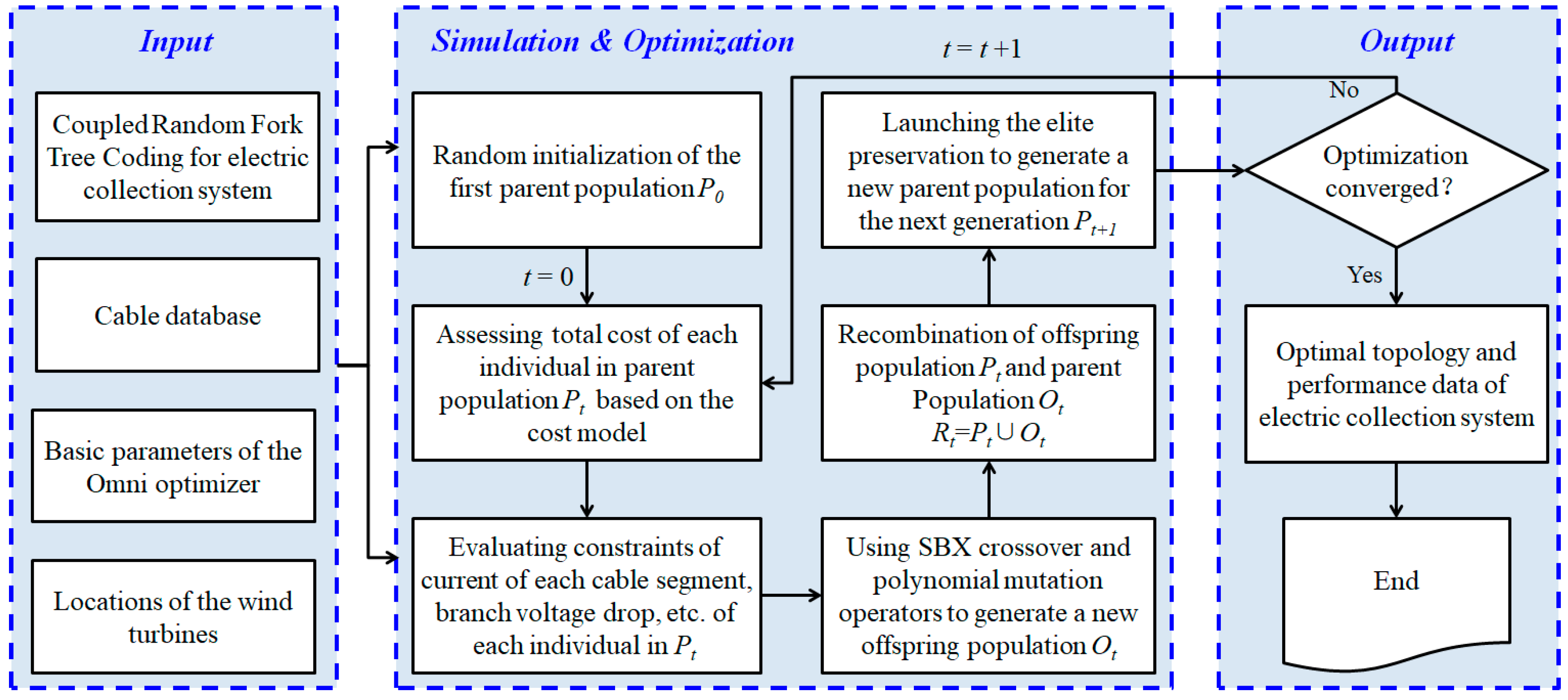
Coupled with the Omni optimizer, the integration optimization framework of the wind farm power collection system is shown in Figure 6, and the specific steps are as follows: First, input of the basic parameters, such as wind turbine coordinates, cables, and algorithms; then, CRFTC was used to encode the variables; randomly generating the initial population, analyzing the generated electrical parameters of the topology, and obtaining the values of the optimization objectives and constraints; using the Omni optimizer’s crossover, mutation, and elite preservation operations to generate a new population; and finally, the convergence condition was judged, and if it converged, the result of the optimization was output; if there was no convergence, the population was updated, and the optimization operation of the t+1 generation was performed.

4. Examples and Discussions

To illustrate the advantages and characteristics of the proposed integrated method over the traditional two-step method, optimizations are carried out for power collection systems in an irregular wind farm containing 40 wind turbines and a regular wind farm containing 51 wind turbines, respectively. The Siemens 3.6 MW wind turbines were selected as energy inputs to the power system, having a rotor with a diameter of 107 m. The design of the two-step method used the most widely used type of current power collection system, i.e., the MST was used to generate the topology, and then the cross section of the cable was distributed according to the current-carrying capacity [5,6,7,8,9,10]. The main electrical parameters in the optimization are given in

Table 1. Main electrical parameters.

Parameter (Unit)	Value
Wind turbine rated power PR (MW)	3.6
Medium voltage network voltage VM (kV)	30
Branch road allowable voltage drop (kV)	1% VM
Power factor of the wind turbine cosφ	0.95

. In the example used, the population size was taken as 100, the largest evolutionary algebra was 5000, and the crossover and mutation rates were 0.9 and 0.01, respectively.

4.1. Comparison of Optimal Schemes in One Substation

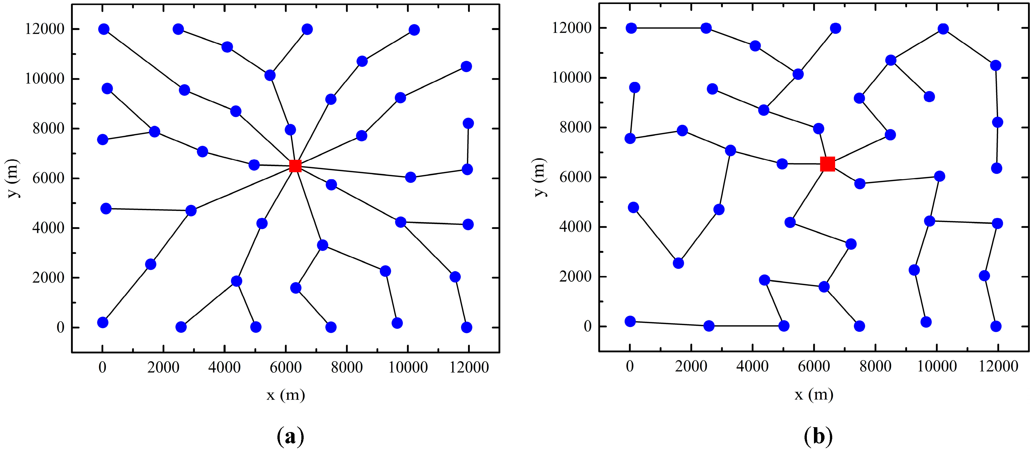
In this scheme, the wind turbines are randomly distributed within the range of 12 km × 12 km, and the distance between any two wind turbines was greater than 10 times the diameter of the wind rotor.

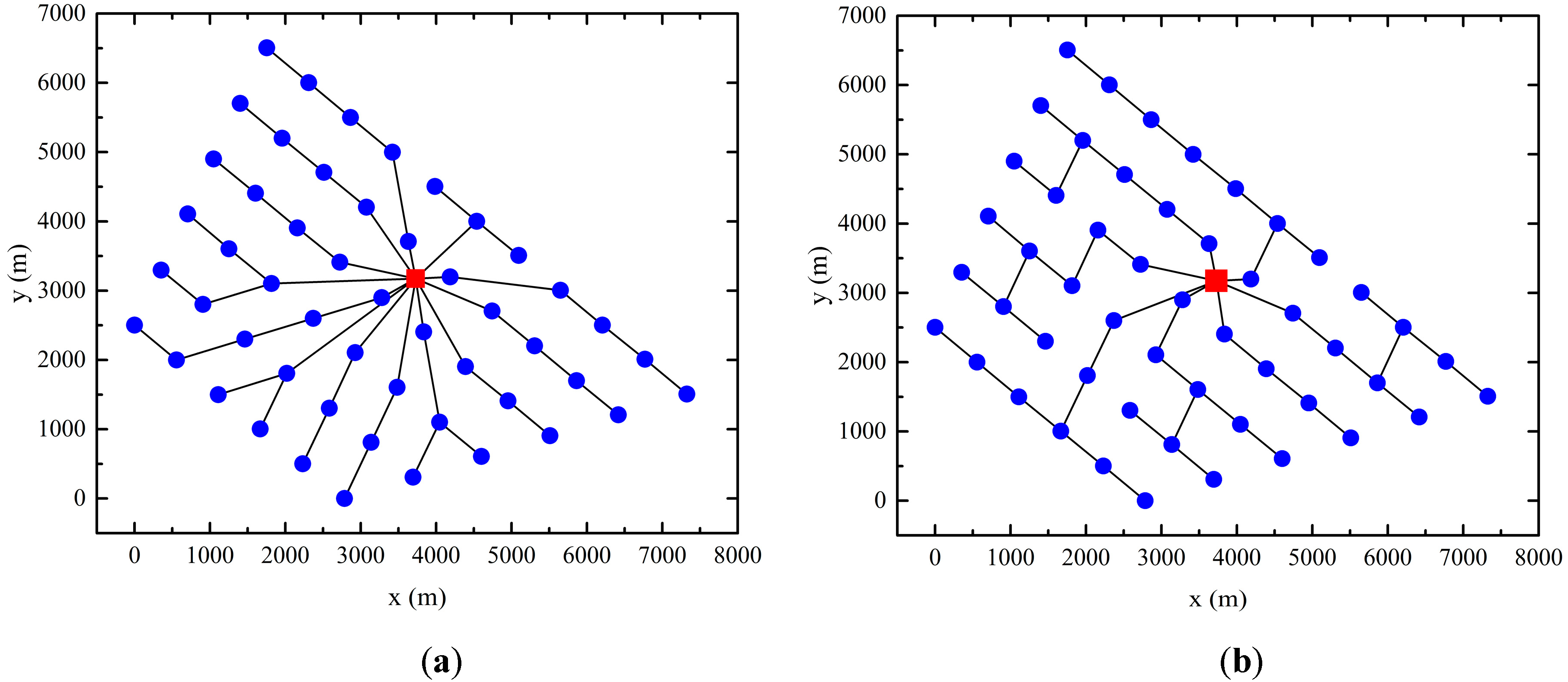
Figure 7 shows the optimal topological comparison of the proposed integration method and the traditional two-step method. In the figure, the blue circles and the red squares represent wind turbines and offshore substations, respectively. The optimal topology obtained by the two methods exhibited significant differences in structure. The optimal topology obtained by the integration method formed ten branches, and the number of wind turbines in each branch was 3, 3, 3, 5, 5, 4, 4, 5, 3, and 5. While the optimal topology obtained by the two-step method formed five branches, the number of wind turbines in all branches was eight.

Table 2. Comparison of key economic parameters of the topology (references for the % are the values obtained by the two-step method).

Type	Intergration Method	Two-Step Method
Total cost Ctotal (million USD)	14.88 (−36.6%)	23.49
Total cable length (km)	92.70 (12.9%)	82.09
Annual energy loss (MWh/a)	4537 (−62.9%)	12251
Medium voltage cable cost (million USD)	7.42 (7.7%)	6.89
Total construction cost (million USD)	1.95 (13.4%)	1.72
Energy loss cost (million USD)	5.51 (−62.9%)	14.88

exhibits the key economic parameters of the optimal topology obtained by the two methods. From the perspective of cost composition, in the topology obtained by the two-step method, the energy-loss cost was the main expenditure part, accounting for 63.3% of the total cost, while the cable cost only accounted for 29.3%, indicating that the traditional cable section design scheme based on the current carrying capacity exhibited serious energy and economic losses. The energy-loss cost of the optimal topology obtained by the integration method was greatly reduced, accounting for only 37% of the total cost. 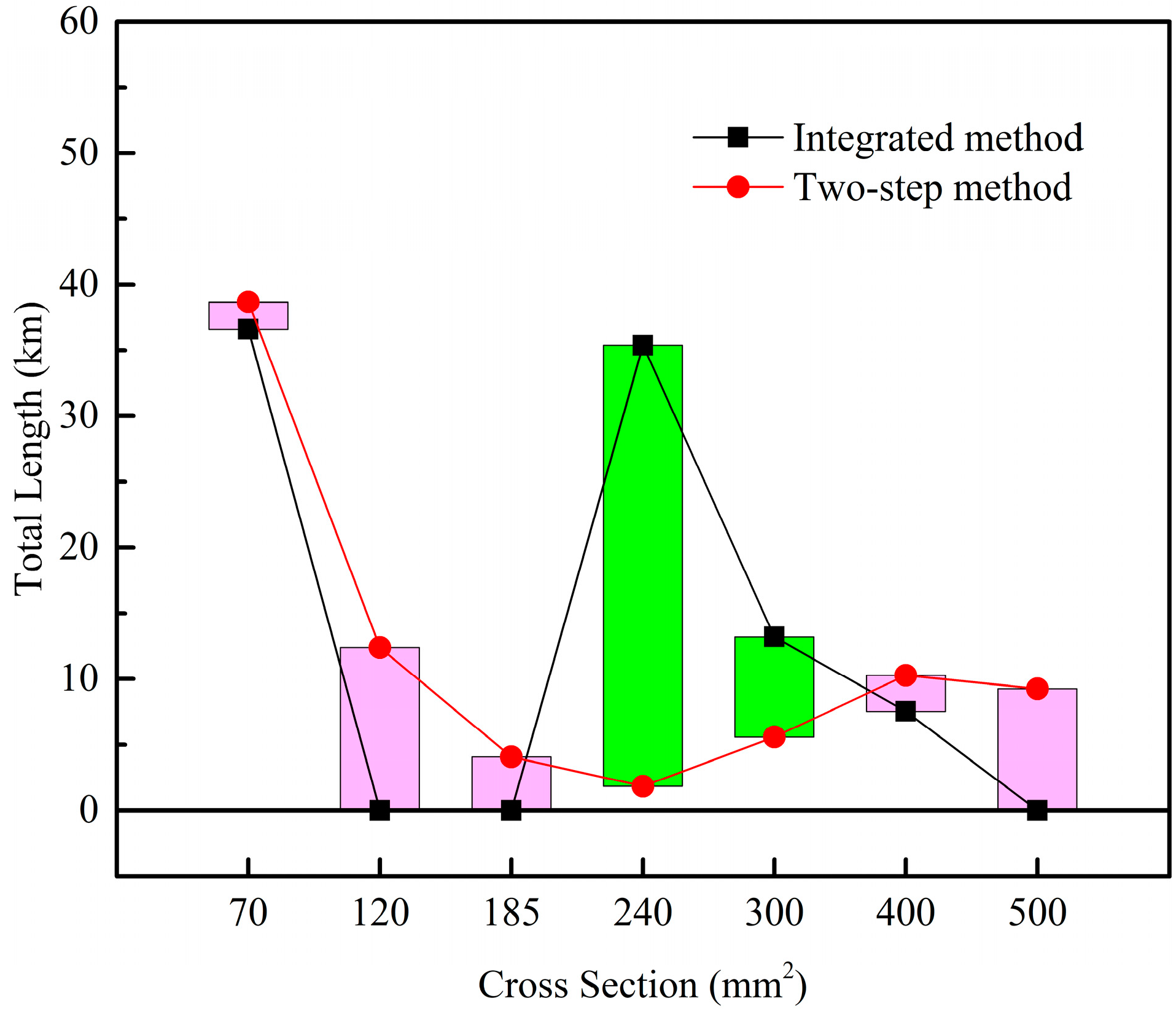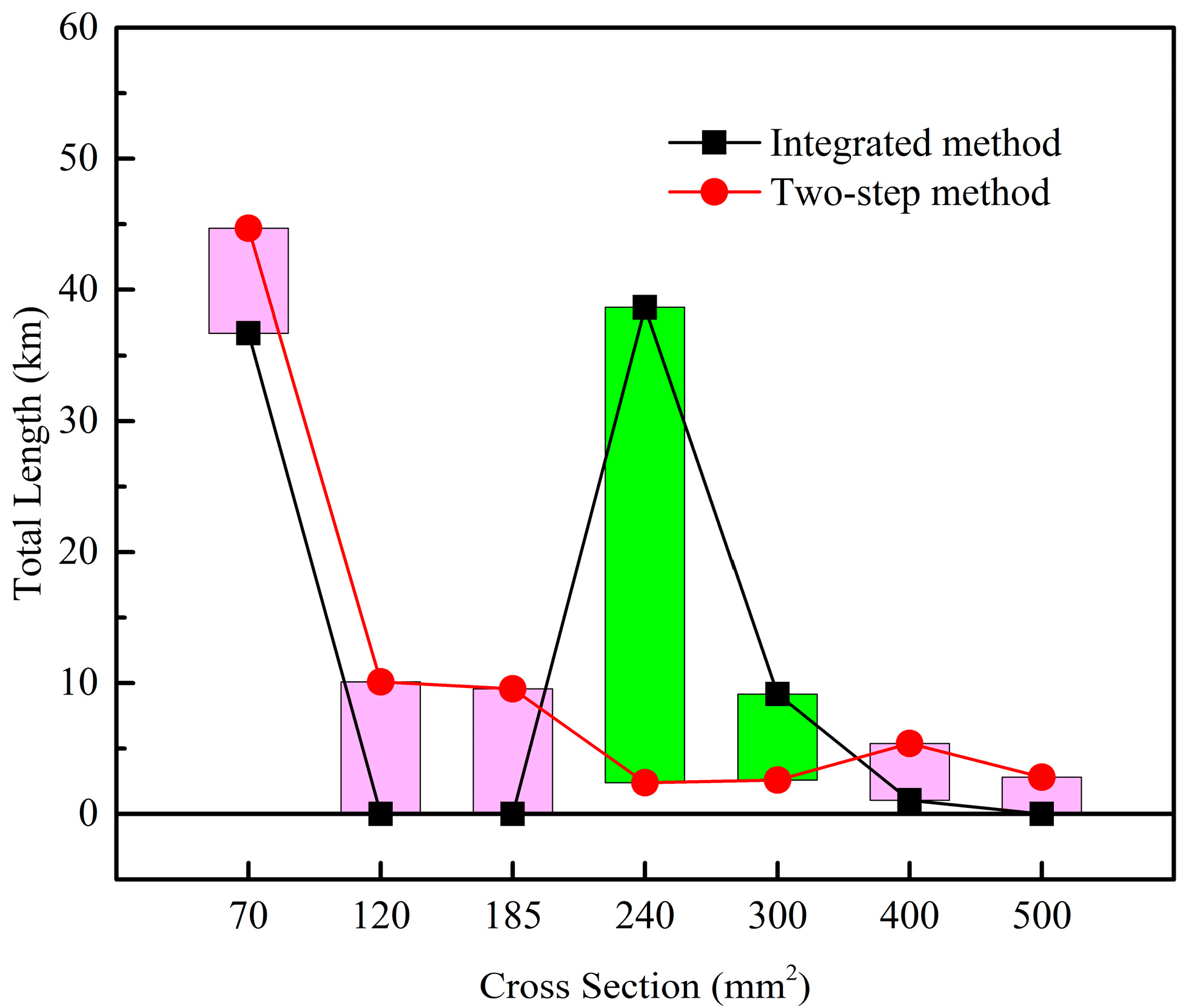Figure 8 shows a comparison of the cable lengths with different cross sections for the optimal topology obtained by the two methods. In the two-step method, the cross section is determined according to the maximum current in each cable segment, thus it is preferred to use small cross-section cables such as 70 mm² and 120 mm² in the construction of the power collection system. In order to reduce the overall resistance level, the large cross-section cables of 240 mm² and 500 mm² are used extensively in the optimal topology obtained by the proposed method. Therefore, the annual energy loss decreases greatly from 12251 MWh/a to 4537 MWh/a, which greatly reduces the energy loss cost. From a comprehensive perspective, although the total length of the cable for the optimal topology was increased by 12.9% and the cost of the medium voltage cable increased by 7.7% when compared to the two-step method, the total cost decreased by 36.6%.

Comparing the optimal topological characteristics of the two methods, the two-step method separated the topology optimization from the cable cross-sectional area planning. First, it aimed to obtain the topology with the shortest total length, so each wind turbine could find and connect the nearest distance wind turbines, until the branch reaches the maximum number of wind turbines. Then, the appropriate cross-sectional area of the cable was allocated according to the current-carrying capacity of the connecting section. In contrast, the integration approach employed the use of more branches to reduce the number of wind turbines in each branch, and also used plenty of large cross-section cables to reduce the energy losses caused by the impedance in the topology. In the optimization process, the integration approach approached the best match of the topology and the cable cross-section to minimize the total cost.

4.2. Comparison of Optimal Schemes in Two Substations

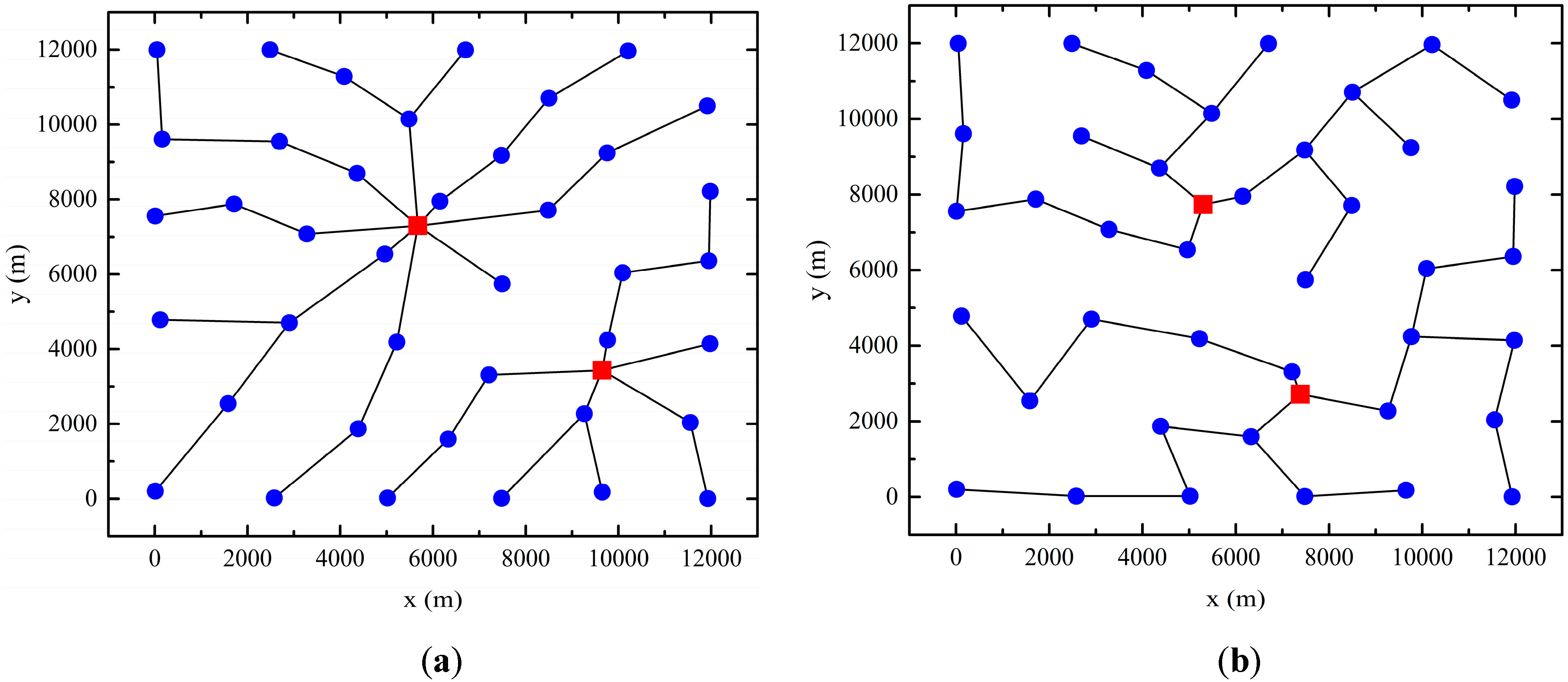
In the case where two substations were arranged in the same wind farm, the optimal topology and economical differences of the power collection system obtained by the proposed integration method and the conventional two-step method were also analysed. Figure 9 indicates an optimized topology comparison obtained by the two methods.

Table 3. Summary of total cable usage and cost (references for the % are the values obtained by the two-step method).

Type	Intergration Method	Two-Step Method
Total cost Ctotal (million USD)	12.50 (−32.3%)	18.47
Total cable length (km)	85.57 (10.4%)	77.50
Annual energy loss (MWh/a)	3519 (−62.6%)	9406
Medium voltage cable cost (million USD)	6.43 (18.9%)	5.41
Total construction cost (million USD)	1.80 (10.4%)	1.63
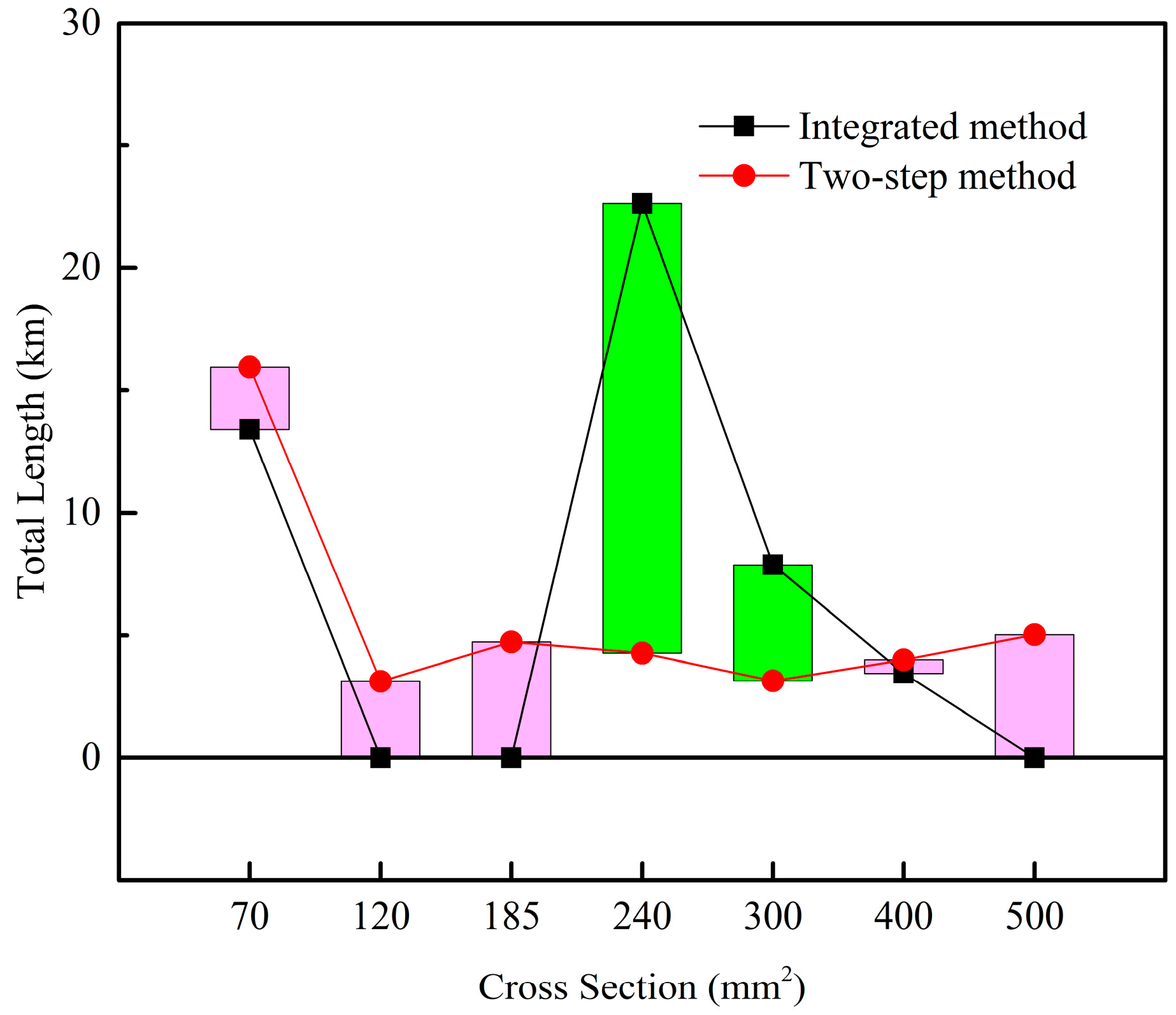
Total energy loss cost (million USD)	4.28 (−62.6%)	11.43

and Figure 10 show the key economic and power parameters for the two methods to obtain the optimal solution, as well as the comparison of cable usage for different cross-sectional areas. The number of branches of the optimal topology obtained by the integration method was more than that of the two-step method (13 and 6, respectively), and there were significant differences in the position of the substation. The total length of the cables with cross sections of 240 mm² or larger in optimal topology obtained by the proposed method is 2.49 times longer than that of the two-step method (Figure 10), resulting in a significant reduction in annual energy loss from 9406 MWh/a to 3519 MWh/a and a reduction in energy-loss cost by 62.6%. Compared to the two-step method, the total length of the cable used by the proposed integrated method was increased by 10.4% to achieve the optimal topology. This resulted in an increase of 18.9% and 10.4% in cable cost and construction cost, respectively. However, due to the large-scale use of the large-section cables, the total cost was greatly reduced by 32.3%.

Comparing one substation condition with two substations’ condition, increasing the number of substations in the optimal topology obtained by the integration method further reduced the development cost of the power system. Besides, the total cost of the two-substation schemes was 21.4% lower than that of the one-substation scheme, the total length of cable used was reduced by 5.6%, and the annual energy loss was reduced by 23.2%.

4.3. Comparison of Optimal Schemes of a Practical Wind Farm

The proposed method is used to optimize the power collection system of a real offshore wind farm called Walney 1. The wind farm is located in the south of the UK and consists of 51 regularly distributed 3.6 MW wind turbines. The substation position is fixed in the wind farm.

Figure 11 and Figure 12 and

Table 4. Summary of total cable usage and cost (references for the % are the values obtained by the two-step method).

Type	Intergration Method	Two-Step Method
Total cost Ctotal (million USD)	8.13 (−34.5%)	12.41
Total cable length (km)	47.37 (17.7%)	40.23
Annual energy loss (MWh/a)	2580 (−60.9%)	6601
Medium voltage cable cost (million USD)	3.99 (12.4%)	3.55
Total construction cost (million USD)	0.99 (17.9%)	0.84
Total energy loss cost (million USD)	3.14 (−60.9%)	8.01

show the comparisons of structures, used cable lengths for the different cross sections, key economic parameters of the optimal topologies obtained by the proposed integration method, and the traditional two-step method. The optimization results are very similar to those of the two examples above. The optimal topology obtained by the proposed method uses 13 branches, more than the 7 branches formed in the optimal topology obtained by the two-step method.

By optimizing the matching between the topology and the cable cross sections, as well as using large cross-section cables reasonably, the annual energy loss of the optimal topology obtained by the proposed method is 2580 MWh/a, much less than 6601 MWh/a obtained by the two-step method, resulting in a 34.5% reduction in the total cost, although the total cable length increases by 17.7%.

In general, the proposed integration method solves the inherent shortcomings of the traditional two-step method, and offers the best solution for the optimal matching of topology, substation location, and cable cross-sectional area. It is also applicable to the power network optimization of wind farms containing any number of wind turbines and substations. Moreover, the proposed method is very versatile and can be combined with any evolutionary algorithm.

4.4. Convergence Performance

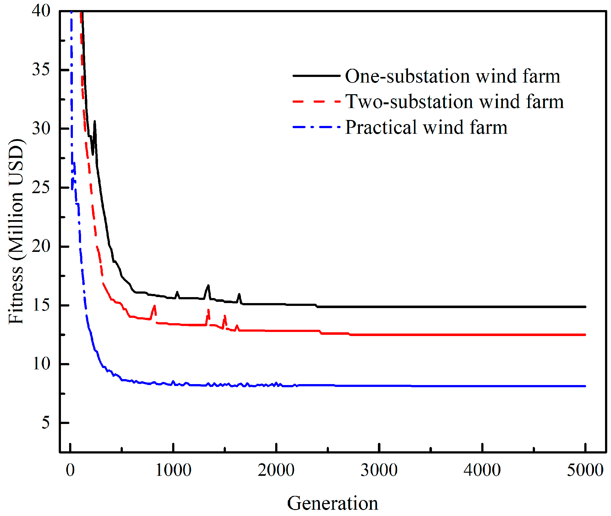
In the launched optimizations of the wind farm power systems, the same calculation is carried out independently five times with different random seeds for each example. After 5000 generations of iteration, the same optimal results of each example were obtained, which proves that the global optimal solution is obtained. The convergence curves for the one- and two-substation schemes as well as the pratical wind farm using the proposed method are shown in Figure 13. All schemes can converge within 3500 generations, indicating good convergence performance. The computations are all done with a single-core processor (Intel Xeon 3.6GHz). The computing time for each generation is about 3 s, and the optimal solution is obtained in about 3 h. These results demonstrate the high optimization efficiency of the proposed integration optimization method.

5. Conclusions

In order to solve the inherent deficiency of the lack of the economical solutions caused by the two-step method of separately optimizing the connection topology and cable planning in the traditional power collection system design, we developed a new integration design method, the proposed coupled random fork tree coding, the union-find set loop identification, and the current and the voltage drop calculation models. The proposed coupling random fork tree coding, for the first time, realized the coupling code of the substation location, connection topology, and cable cross sections, providing the basis for the integration design of the power collection system. Based on this method, an optimization study was carried out on a power collection system of a discrete wind farm and a regular wind farm. The results show that the proposed integration method demonstrated the ability to achieve the best match of topology, substation location, and cable cross-sectional area, and employed more branches, thus reducing the number of wind turbines in each branch. In addition, the integrated approach also used a large cross-sectional area cable to reduce the energy loss caused by the impedance in the topology, and even if the cable cost was increased slightly, the total cost was minimized. In the optimization studies of wind farms containing one substation and two substations, as well as the real wind farm, the total cost of the optimal topology obtained by the integrated method was reduced by 34.3%, 36.4%, and 24%, respectively. Furthermore, the energy loss costs were significantly reduced by 67.4%, 72.1%, and 56.2%, respectively.

Compared with traditional two-step methods, the proposed integration method can achieve the best match of topology, substation location, and the cable cross sections, and deliver the most economical power network optimization solution. In addition, the proposed integration method is very versatile and can be combined with any evolutionary algorithm. Besides, it is suitable for the optimal design of power collection systems including any number of wind turbines and substations.