Abstract
Performing numerous simulations of a building component, for example to assess its hygrothermal performance with consideration of multiple uncertain input parameters, can easily become computationally inhibitive. To solve this issue, the hygrothermal model can be replaced by a metamodel, a much simpler mathematical model which mimics the original model with a strongly reduced calculation time. In this paper, convolutional neural networks predicting the hygrothermal time series (e.g., temperature, relative humidity, moisture content) are used to that aim. A strategy is presented to optimise the networks’ hyper-parameters, using the Grey-Wolf Optimiser algorithm. Based on this optimisation, some hyper-parameters were found to have a significant impact on the prediction performance, whereas others were less important. In this paper, this approach is applied to the hygrothermal response of a massive masonry wall, for which the prediction performance and the training time were evaluated. The outcomes show that, with well-tuned hyper-parameter settings, convolutional neural networks are able to capture the complex patterns of the hygrothermal response accurately and are thus well-suited to replace time-consuming standard hygrothermal models.
1. Introduction
When simulating the hygrothermal behaviour of a building component, one is confronted with many uncertainties, such as those in the exterior and interior climates, in the material properties, or even in the configuration geometry. A deterministic assessment does not enable taking into account these uncertainties, and as such, often does not allow for a reliable design decision or conclusion. A probabilistic analysis [1,2,3,4,5,6], on the other hand, enables including these uncertainties, and thus allows a more reliable assessment of the hygrothermal performance and the potential moisture damages. For this purpose, usually, the Monte Carlo approach [7] is adopted, where the uncertain input parameters’ distributions are sampled multiple times and a deterministic simulation is executed for each sampled parameter combination. This approach often involves thousands of simulations and therefore, easily becomes computationally inhibitive. To surmount this problem, the hygrothermal model can be replaced by a metamodel, which is a simpler and faster mathematical model mimicking the original model, thus strongly reducing the calculation time. Static metamodels have already been applied in the field of building physics multiple times [8,9,10]. The main disadvantage is that these types of metamodels are developed for a specific single-valued performance indicator (e.g., the total heat loss or the final mould growth index). The wish to use a different performance indicator would require the construct of a new metamodel, which is time-intensive. Additionally, single-valued performance indicators provide less information, which might impede decision-making. For example, the maximum mould growth index is calculated based on the temperature and relative humidity time series and shows the maximum value over a period, but does not allow for assessing how long or how often this maximum occurs, or how high the mould growth index is the rest of the time.
Dynamic metamodels, on the other hand, aim to predict actual time series (temperature, relative humidity, moisture content, etc.), and thus provide a more flexible approach. Predicting the hygrothermal time series allows post-processing by any desired damage prediction model (e.g., the mould growth index), as well as provides information over the whole period. Using a metamodel to predict time series, rather than single-value performance indicators, is, to the authors’ knowledge, new to the field of building physics. However, it is also more difficult, as the metamodel must be able to capture the complex and time-dependent pattern between input and output time series, and not all metamodeling strategies are suited for time series prediction.
In a previous study [11], the authors demonstrated that neural networks are well-suited to reproduce the dynamic hygrothermal response of a building component. Three popular types of neural networks were considered: multilayer perceptrons (MLP), the long-short-term memory network (LSTM) and the gated recurrent unit network (GRU), both of which are a type of recurrent neural network (RNN), and convolutional neural network (CNN). These networks were trained to predict the hygrothermal time series such as temperature, relative humidity and moisture content at certain positions in a masonry wall, based on the time series of exterior and interior climate data. The results showed that a memory mechanism to access information from past time steps is required for accurate prediction performance. Hence, only the RNN and the CNN were found to be adequate. Furthermore, the CNN was shown to outperform the RNN and was also much faster to train.
This study builds upon these previous findings. As the CNN was found to perform best, it is developed further, aiming to replace HAM-simulations (HAM: Heat, Air and Moisture) for a spectrum of facade constructions (with different geometry and materials) and/or boundary conditions (with varying exterior and interior climate, orientation, wind-driven rain, etc.). During development, many parameters inherent to the neural network architecture and training process—called the hyper-parameters—need to be defined though. Considering that these parameters can significantly influence the network’s performance, it is important to choose the most optimal combination. However, this is usually a trial-and-error process, as there are no general guidelines. This paper hence proposes an approach to optimise these hyper-parameters, using the Grey-Wolf Optimisation (GWO) algorithm, as it was found competent for other applications [12,13]. This is applied to a one-dimensional (1D) brick wall, of which, the hygrothermal performance is evaluated for typical moisture damage patterns.
The next section first presents the architecture of the convolutional neural network. Next, the hyper-parameters optimisation method is explained, after which, the networks’ performance evaluation is described. Section 3 describes the application and calculation object and in Section 4, the results of the hyper-parameter optimization and the networks’ performance are brought together and discussed. In the conclusions, the main findings are summarised, and some final remarks are drawn.
2. Optimising Convolutional Neural Networks (CNN)
2.1. The Network Architecture
Convolutional neural networks are a class of deep neural networks most commonly applied to image analysis. More recently though, CNNs have been applied to sequence learning as well [11,14,15]. A convolution is a mathematical operation on two functions to produce a third function, defined as the integral of the product of these functions after one is reversed and shifted. In the case of a CNN, the convolution is performed on the input data and a weights array, called the filter, to then produce a feature map. The filter actually slides over the input, and at every time step, a matrix multiplication is performed. This is repeated for each input parameter (feature) and the result is summed into a new feature map. In case of sequences or time series, often dilated causal convolutions are used. Causal means that the output of the filter does not depend on future input time steps. Dilated means that the filter is applied over a range larger than its length by skipping input time steps with a certain step. By stacking dilated convolutions, the network can look further back into history (i.e., the receptive field) with just a few layers, while still preserving the input resolution throughout the network (i.e., the number of time steps in the sequence) as well as the computational efficiency. Often, each additional layer increases the dilation factor exponentially, as this allows the receptive field to grow exponentially with the network depth. This principle is shown in Figure 1 for a filter width of two time-steps.
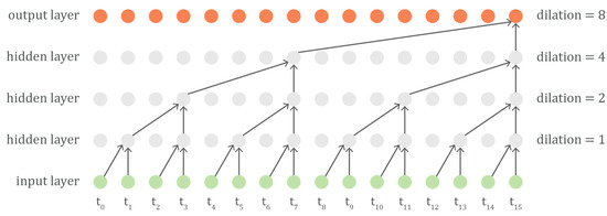
Figure 1.
The causal dilated convolutions allow an output time step to receive information from a larger range of input time steps (i.e., the receptive field) with an increasing number of hidden layers. In the presented scheme, a filter width of two, four layers and one stack results in a receptive field of sixteen input steps.
The architecture of the CNN network used in this paper, shown in Figure 2 is based on the Wavenet architecture [16] and is developed using Keras 2.2.4 [17]. The network consists of stacked ‘residual blocks’, followed by two final convolutional layers. By layering multiple residual blocks, a larger receptive field is obtained. The dilation can be exponentially increased for a number of layers and then repeated, e.g., 20, 21, 22, …, 29, 20, 21, 22, …, 29, 20, 21, 22, …, 29, for filter width two. These repetitions of layered residual blocks are called stacks. The combination of the filter width, number of layers and number of stacks defines the length of the receptive field.
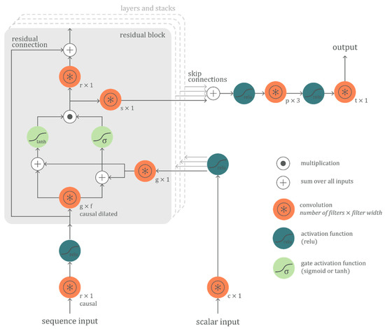
Figure 2.
The used convolutional neural networks (CNN) architecture with residual blocks, skip connections and global conditioning, based on the Wavenet architecture.
Each residual block contains three important elements that give the network its prediction strength: a gated activation unit, residual and skip connections and global conditioning. The gated activation unit starts with a causal dilated convolution, which then splits, passes through either a tanh or sigmoid activation and finally recombines via element-wise multiplication. The tanh activation branch can be interpreted as a learned filter and the sigmoid activation branch as a learned gate that regulates the information flow from the filter [18]. Recurrent neural networks such as the Long Short-Term Memory (LSTM) and Gated Recurrent Unit (GRU) use similar gating mechanisms to control the flow of information. The gated activation unit can mathematically be represented by Equation (1), where, corresponds to the learned dilated causal convolution weights and and denote filter and gate, respectively:
The skip connections allow lower level signals to pass unfiltered to the final layers of the network. Hence, earlier feature layer outputs are preserved as the network passes forward signals for final prediction processing. This allows the network to identify different aspects of the time series, i.e., strong autoregressive components, sophisticated trend and seasonality components, as well as trajectories difficult to spot with the human eye. Residual connections allow each block’s input to bypass the gated activation unit, and then add that input to the gated activation unit output. This helps allow for the possibility that the network learns an overall mapping that acts almost as an identity function, with the input passing through nearly unchanged. The effectiveness of residual connections is still not fully understood, but a compelling explanation is that they facilitate the use of deeper networks by allowing for more direct gradient flow in backpropagation [19].
Finally, global conditioning allows the network to produce output patterns for a specific context. For example, if different brick types are included, the network can be trained by feeding it the brick characteristics as additional input. In this case, the gated activation unit can mathematically be represented by Equation (2), where, corresponds to the learned convolution weights and is a tensor that contains the conditional scalar input and is broadcast over the time dimension:
2.2. Hyper-Parameter Optimization
In order to configure and train the network, the hyper-parameters of the network need to be set. For configuring the proposed architecture (Figure 2), these are:
- Filter width f of causal dilated convolution
- Number of c-filters for initial conditional connection
- Number of g-filters for gate connections
- Number of s-filters for skip connections
- Number of r-filters for residual connections
- Number of p-filters for the penultimate connection
- Number of layers of residual blocks
- Number of stacks of layered residual blocks
Additionally, there are hyper-parameters concerning the training process itself:
- Loss function
- Learning algorithm
- Learning rate
- Number of training epochs
- Batch size
The loss function is minimised during training by determining the neurons’ optimal weights and is a measure of how good the network fits the data. In this optimisation, the root-mean-squared-error (RMSE) is used as the loss function, because it effectively penalises larger errors more severely. The learning algorithm defines how the neurons’ weights are updated during the learning process. Many learning algorithms exist, but in this study, the Adam algorithm [20] is used, as the authors’ previous experiments showed it to perform best for the current problem. The learning rate is the allowed amount of change to the neurons’ weights during each step of the learning process. At extremes, a learning rate that is too large may result in too-large weight updates, causing the performance of the network to oscillate over training epochs. A too-small learning rate may never converge or may get stuck on a suboptimal solution. The learning rate must thus be carefully configured. The batch size is the number of training samples passed through the neural network in one step. The larger the batch size, the more memory is required during training. As the networks are trained on a computer with two NVIDIA RTX 2070 GPU’s, each with 8 GB RAM, the available memory is limited. For this reason, the batch size is fixed to four samples. After each batch, the network’s weights are updated. When all batches have passed through the network once, one training epoch is completed. The number of training epochs is the number of times the entire training dataset is passed through the neural network. The more often the network is exposed to the data, the better it becomes at learning to predict. However, too much exposure can lead to overfitting: the network’s error on the training data is small but when new data is presented to the network, the error is large. This is prevented by stopping training if the error on the validation dataset no longer decreases, a mechanism called ‘early stopping’.
To reduce the training time during the optimisation process, two measures are taken: Firstly, the training set contains only 256 samples, which reduces the number of batches in each epoch. Secondly, each neural network is trained for a maximum of only 50 epochs, and training is stopped earlier if the RMSE on the validation set (containing 64 samples) decreases less than 0.001 over 5 epochs. These measures reduce training time successfully, but do not allow for reaching the best prediction performance, as both the number of epochs and the number of samples in the training set are too small. However, this approach allows for identifying the hyper-parameter combinations that converge fastest and are thus likely to perform best. Table 1 gives an overview of all hyper-parameters that need to be fine-tuned, in order to get optimal prediction results. Because evaluating all possible combinations in a full factorial way would be extremely expensive, optimization of these hyper-parameters is done via the Grey-Wolf Optimiser (GWO) [12]. It is a population-based meta-heuristic based on the leadership hierarchy and hunting mechanism of grey wolves in nature. Grey wolves live in a pack in which alpha (α), beta (ß), delta (δ) and omega (ω) wolves can be identified. Positioned on top of the pack, the α-wolf decides on the hunting process and other vital activities. The other wolves should follow the α-wolf’s orders. The ß-wolves help the α-wolf in decision-making. The δ-wolves have to submit to the α- and ß-wolves, but dominate the ω-wolves, who are considered the scapegoats of the pack. In the GWO, the fittest solution is considered as α, and the second and third fittest solutions are named ß and δ, respectively. The rest of the solutions are ω. In search of the optimal solution, the α-, ß-, and δ-solutions guide the direction, and the ω-solutions follow. The three best solutions are saved and the other search agents (ω) are obligated to update their positions according to the positions of the best search agents.

Table 1.
The search range of the hyper-parameters.
In this study, 10 search agents are deployed to explore and exploit the search space over 100 iterations. If the best solution does not change for 25 iterations, the search algorithm is stopped. This is repeated for five independent runs as different runs might end with different optimal solutions. The RMSE on the validation set is used to evaluate the fitness of the solutions.
2.3. Performance Evaluation
Once the GWO algorithm has finished, the ten best solutions (lowest RMSE) of all runs are trained fully to reach the networks’ full prediction potential, by using a training set of 768 samples, with a validation set of 192 samples. A maximum of 200 epochs is set, with early stopping if the RMSE decreases less than 0.001 over 20 epochs. Each combination is trained five times, to overcome initialisation differences. Note that the size of the training dataset is chosen rather arbitrarily: this is based on previous experiments, showing that training on 786 samples resulted in better prediction performance compared to 256 training samples (for identical hyper-parameters). These numbers might not be optimal, i.e., a larger dataset might result in even better prediction performance or vice versa, a smaller dataset might provide equally satisfying results.
The performance of these 10 fully-trained neural networks is evaluated using three performance indicators: the root mean-square error (RMSE), the mean absolute error (MAE), and the coefficient of determination (R2), quantified as follows:
where, is the true output, is the predicted output, is the mean of the true output and is the total number of data points. Additionally, the models’ training time is evaluated.
Finally, the best performing network, defined as the one with the lowest RMSE on the validation dataset (192 samples), is selected. Because performance on the validation dataset is incorporated into the network’s hyper-parameter optimisation, this final network’s performance is tested using an independent test set, containing 256 samples. This way, an unbiased performance evaluation is obtained. The performance indicators are calculated for each target separately, to identify which targets are more or less accurately predicted. Subsequently, the network’s output is used to predict the damage risks. These results are evaluated using the same performance indicators as described above.
3. Application
3.1. Hygrothermal Simulation Object
The calculation object in this study is a 1D cross-section of a massive masonry wall. The masonry wall is simplified to an isotropic brick layer—no mortar joints are modelled [21]—and an interior plaster layer of 1.5 cm. Note that no construction details, such as corners or embedded beams, are modelled.
To explore the capabilities of the proposed convolutional neural network, all characteristics and boundary conditions that are expected to significantly influence the hygrothermal performance of the 1D wall are considered probabilistic (Table 2). Variability in climatic conditions is included by using different years of climate data of four Belgian cities [22]. Since the aim is to predict the expected future performance of the wall, future climate data is used. Variability in the wall conditions is incorporated via uniform distributions of the wall orientation, solar absorption and exposure to wind-driven rain. The wind-driven rain load is calculated by using the catch ratio, as described in Reference [23]. The catch ratio relates the wind-driven rain (WDR) intensity on a facade to the unobstructed horizontal rainfall intensity and is a function of the reference wind speed and the horizontal rainfall intensity for a given position on the building facade and wind direction. In this model, variability in wall position and potential shelters, trees or surrounding buildings are reckoned with by the exposure factor. Additionally, the transiency and variation of the wind speed is taken into account in the convective heat transfer coefficient, via Equation (4) (EN ISO 06946), where, and .
Table 2.
Probabilistic input parameters and distributions.
The exterior moisture transfer coefficient is related to the exterior heat transfer coefficient through the Lewis relation. The interior climate is calculated according to EN 15026 [24] and variability in building use is included by using two different humidity loads. Finally, to explore the CNN’s capabilities to the maximum, three different brick types as well as a uniform distribution of the wall thickness are included as well. The basic characteristics of the used brick types can be found in Table 3 and Figure 3, which clearly show the variations in the bricks’ moisture properties.
Table 3.
Brick type characteristics.
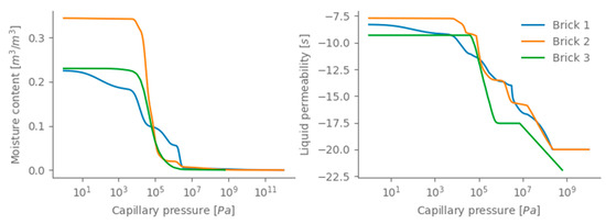
Figure 3.
Brick type moisture properties; (left)the moisture retention curve and (right) the liquid permeability.
The remaining parameters are all variables either with small variations or of less importance for the current study of a 1D wall. Therefore, these boundary conditions are assumed deterministically. Table 4 gives an overview of the deterministic boundary conditions.
Table 4.
Discrete input parameters.
When evaluating the hygrothermal performance of a massive masonry wall, one is typically interested in frost damage at the exterior surface, decay of embedded wooden floors and mould growth on the interior surface [3,25,26,27]. The latter is mainly important in the case of thermal bridges and of less importance in 1D simulations. Table 5 gives an overview of frequently used prediction models for these damage patterns, and the required hygrothermal time series to evaluate them. Figure 4 schematically presents the two-dimensional (2D) building component (top) and the modelled 1D mesh (bottom) and indicates at which positions the hygrothermal performance is monitored. The simulations were performed using the hygrothermal simulation environment Delphin 5.8 [28], and a simulation period of four years was adopted. As most damage prediction models require hourly data, an hourly output frequency is used.
Table 5.
Damage prediction models and required Delphin output.
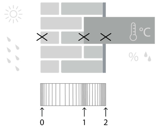
Figure 4.
A schematic representation of the two-dimensional (2D) building component (top) and the modelled one-dimensional (1D) mesh (bottom), with indication at which positions the hygrothermal performance is monitored.
The frost damage risk is evaluated via the number of moist freeze-thaw cycles at 0.5 cm from the exterior surface. A ‘moist’ freeze-thaw cycle is a freeze-thaw cycle that occurs in combination with a moisture content high enough to induce frost damage [3]. In this study, the critical moisture content is defined as a moisture content above 25% of the saturated moisture content. Note that this is a rather arbitrary value, as currently no precise prediction criterion is at hand. An indication of the decay risk of wooden beam ends can be made using the VTT wood decay model, which calculates the percentage of mass loss of the wooden beam end based on the temperature and relative humidity [29]. Note, however, that in this 1D wall study, solely a rough indication of the wood decay risk is acquired, as two- and three-dimensional heat and moisture transport, as well as potential air rotations around the wooden beam end, are neglected [30]. At the interior surface, a too-high relative humidity entails a risk on mould growth. The mould growth risk can be estimated by the VTT mould growth model, which calculates the Mould Index based on the fluctuation of the temperature and relative humidity [31]. The Mould Index is a value between 0 and 6, going from no growth to heavy and tight mould growth. In the updated VTT model, the expected material sensitivity to mould growth is implemented as well. In this study, the materials are assumed to belong to the class ‘very sensitive’.
3.2. Training the Convolutional Neural Network
The training and validation datasets are obtained by sampling the input parameters described above multiple times, using a Sobol sampling scheme [32], and simulating the deterministic HAM model once for each sampled input parameter combination. In this study, in total, 960 samples are used. The network is trained to predict hygrothermal time series as requested for the damage prediction models (see Table 5), based on the input in Table 2 and Table 3. The inputs are pre-processed to facilitate learning. The scalar parameters ‘wall orientation’, ‘exterior heat transfer coefficient slope’, ‘solar absorption’ and ‘rain exposure’ are integrated in the exterior climate time series but also preserved as a separate scalar input parameter, to condition the network (see Figure 2). The categorical parameters ‘start year’ and ‘interior humidity load’ are incorporated into the climate time series. The categorical parameter ‘brick type’ is replaced by scalar parameters of the characteristics in Table 3. This simplifies the network architecture and allows more flexibility on using brick types with differing characteristics. This results in 6 input time series (exterior temperature, exterior relative humidity, wind-driven rain load, short-wave radiation, interior temperature and interior relative humidity) and 10 scalar inputs (exterior heat transfer coefficient slope (Equation (4)), rain exposure factor, solar absorption, wall orientation, brick wall thickness and the 5 brick characteristics from Table 3.
Before presenting the input and output data to the neural network, all data are standardised (zero mean, unit variance). This ensures that all features are on the same scale, which allows weighting all features equally in their representation. Standardising the output data ensures that errors are penalised equally for all targets.
4. Results and Discussion
4.1. Hyper-Parameter Optimization
The results of the hyper-parameter optimization show that some (combinations of) parameters have a significant influence on the network’s performance, while others are less important. Figure 5 shows the RMSE on the validation dataset of all GWO candidate solutions, in function of the receptive field and the filter width of the causal dilated convolution. This figure clearly shows that a receptive field of at least 14 months (10,224 h) is required to obtain a low RMSE. The length of the receptive field is defined by the filter width, number of layers and number of stacks, and determines how many past-input time steps the network can use to predict the current output time step. Hence, it makes sense that the receptive field has a threshold below which the network does not perform well, as it cannot access enough information. Figure 5 also shows that a low RMSE can be obtained for all filter widths. Note that this is not the case for filter widths below five, as these require a large number of layers and stacks (cfr. receptive field), which caused out-of-memory errors on the used hardware. If more GPU memory is available, one might not run into this problem. Additionally, Figure 6 (top) shows that using multiple stacks results in a slightly lower RMSE, compared to only one stack. Adding extra stacks to the network allows for increasing the depth—and thus the complexity of the model—without increasing the receptive field exponentially. Indeed, if the receptive field becomes much larger than the actual time series length, the computational efficiency decreases. On the other hand, Figure 6 (top) also shows that the training time increases with the number of stacks. The number of layers has a similar influence on the training time (not shown here), but not on the prediction performance, provided that the receptive field is large enough. Hence, if the number of stacks were fixed, a large filter width would require fewer layers and thus shorter training time, compared to a smaller filter width, while both options would yield similar prediction performance.
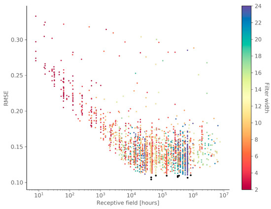
Figure 5.
This scatterplot of all Grey-Wolf Optimiser (GWO) candidate solutions shows that a receptive field of at least 14 months (10,224 h) is required to obtain a low root mean-square error (RMSE) on the validation set, and that a low RMSE can be obtained for all filters widths, once above this receptive field threshold. The 10 best solutions are indicated in black.
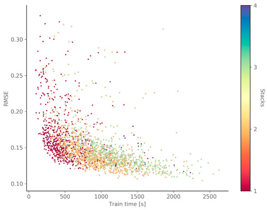
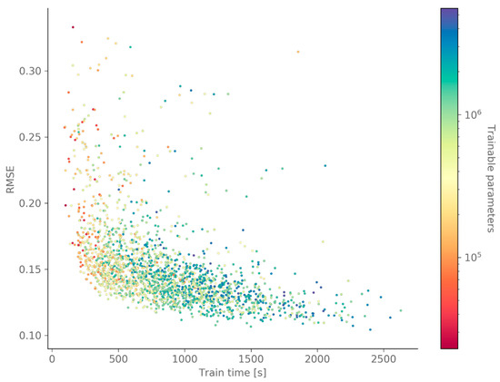
Figure 6.
This scatterplot of all GWO candidate solutions shows a clear relation between the performance (RMSE), the training time and the number of stacks (top) or the number of parameters (determined by the number of layers, stacks and filters) (bottom).
Regarding the number of filters for the different connections, some tendencies can be observed in Figure 7 but there appears to be no clear relationship with the validation RMSE—with the exception that 32 filters is too few for all connections. However, the number of filters has a significant impact on the training time, as shown by Figure 6 (bottom). Combined with the filter width and the number of layers and stacks, the number of filters determines the number of trainable parameters. Hence, using fewer filters, for the same combination of filter width, layers and stacks, generally results in a lower training time.
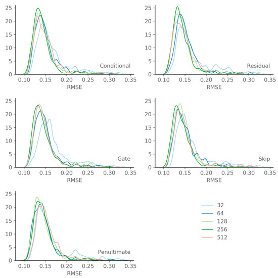
Figure 7.
This distribution plot of all GWO candidate solutions shows some tendencies but no clear relation between the number of filters and the RMSE on the validation set.
Finally, Figure 8 indicates that the optimal learning rate for networks with larger filter widths is around 0.0015, whereas networks with smaller filters widths (i.e., deeper networks) seem to perform better with a larger learning rate around 0.003.
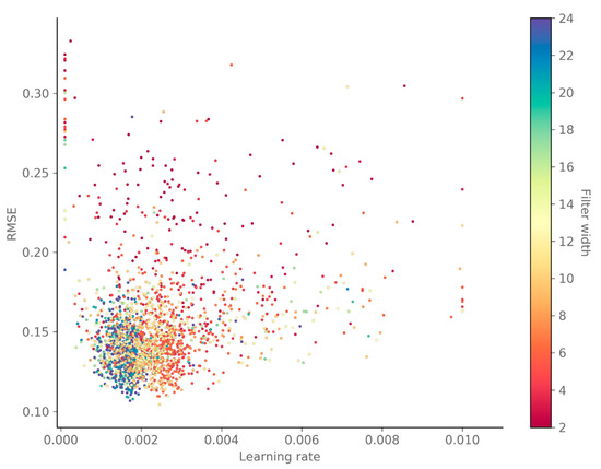
Figure 8.
This scatterplot of all GWO candidate solutions shows that the optimal learning rate depends on the used filter width: larger filter widths require smaller learning rates.
4.2. Performance Evaluation
The ten best solutions of the Grey-Wolf Optimiser algorithm are shown in Table 6. and confirm the overall findings described above. The performance indicators of training five repetitions of these ten combinations on the entire training dataset are shown in Figure 9. The results indicate that no single hyper-parameter combination performs significantly better than the others. As long as the receptive field is large enough (14 months), the network is deep enough (2 stacks) and the learning rate is in the range (0.0015; 0.003), the other hyper-parameters appear to have only a minor influence on the prediction performance. Furthermore, due to weight and bias initialisation differences, training a network with identical hyper-parameters twice does not necessarily result in the same prediction performance, as can be observed in Figure 9. Hence, it is best to repeat training a few times, and select the best performing network afterwards. Figure 9 also confirms that, in general, deeper networks with more layers are slower to train. Finally, note that increasing the maximum number of training epochs and the size of the training dataset resulted in a much lower RMSE, compared to the results obtained by the GWO algorithm. This underlines the importance of a representative training dataset, as well as allowing enough training iterations.
Table 6.
The ten best performing solutions of the Grey Wolf Optimiser algorithm.
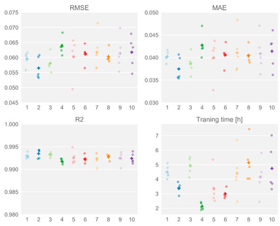
Figure 9.
The performance indicators and training time for the ten best-performing hyper-parameter combinations, after being trained fully. For each combination, the dots indicate each repetition’s result, whereas the cross indicates the average over all five repetitions.
Model 2 performs best on average, but one repetition of model 5 performs better than all other models. Hence, this model’s performance is evaluated using the independent test set. Figure 10 shows an example of a test set sample prediction. The performance indicators shown above each panel are calculated on the standardised output for each target separately, as this indicates the difference in accuracy between targets. It is clear that the chosen network is able to predict all hygrothermal outputs quite accurately. These hygrothermal predictions can be used to evaluate damage risks, as described in Section 3.1. Figure 11 shows the damage predictions (orange) using the networks’ output (for the sample shown in Figure 10), which are in almost perfect agreement with the damage predictions from the Delphin simulations (blue). By expressing the damage risks as single values, it is possible to show the damage prediction accuracy of all individual samples (Figure 12, top) and the cumulated distributions (Figure 12, bottom). The latter is a common presentation in a probabilistic assessment, as it gives information on the distribution of the expected performance taking into account all uncertainties. The frost damage risk is given by the total number of moist freeze-thaw cycles at the end of the simulated period, the mould growth risk on the interior surface is expressed as the maximum mould index over the whole simulated period and the wood decay risk is expressed as the total wood mass loss at the end of the simulated period. Figure 12 shows that the damage risk prediction, based on the networks’ hygrothermal predictions, is quite accurate for most samples of the test set. The number of moist freeze-thaw cycles tends to be overestimated, due to small prediction errors in the temperature and relative humidity. A slightly lower temperature and/or relative humidity at one time step can lead to counting more freeze-thaw cycles compared to the true value. However, both the original hygrothermal model and the neural network predict a low number of moist freeze-thaw cycles, and a difference of a few cycles will likely not much influence the extent of the expected damage. In case of the mould index at the interior surface, the deviations are so small they are negligible. The wood decay risk tends to be slightly underestimated, but the overall agreement in cumulative distribution function is very good.
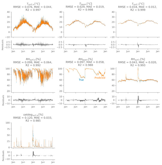
Figure 10.
The network’s hygrothermal predictions (orange) of a test set sample with high accuracy. The true value is shown in blue the prediction error is indicated in grey.
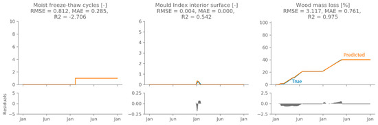
Figure 11.
The damage predictions (orange) for the sample from Figure 10, using the network’s hygrothermal predictions. The true value is shown in blue the prediction error is indicated in grey.
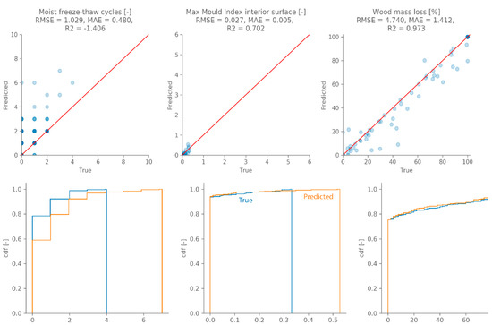
Figure 12.
A comparison between the single-value damage predictions, as obtained using the network’s predictions and the true damage predictions. The top panel shows the goodness-of-fit for the individual samples (transparency is used to indicate overlapping samples), the bottom panels show the cumulated distribution functions.
5. Conclusions
In this paper, convolutional neural networks were used to replace HAM models, aiming to predict the hygrothermal time series (e.g., temperature, relative humidity, moisture content). A strategy was presented to optimise the networks’ hyper-parameters, using the Grey-Wolf Optimiser algorithm and a limited training dataset. This approach was applied to the hygrothermal response of a massive masonry wall, for which the prediction performance and the training time were evaluated. Based on the GWO optimisation, it was found that the receptive field—defined by the filter width, number of layers and number of stacks—has a significant impact on the prediction performance. For the current case study of massive masonry exposed to driving rain, it needs to span at least 14 months. The results also showed that good performance can be obtained for all filter widths, as long as the receptive field is large enough. Additionally, using multiple stacks resulted in slightly better performance compared to a single stack, as this allows adding complexity to the model, but also resulted in longer training time. The number of layers, determined by the filter width and the number of stacks to obtain a large enough receptive field, had a similar influence on the training time, but not on the prediction performance. Hence, if the number of stacks were fixed, a large filter width would require fewer layers and thus shorter training time, compared to a smaller filter width, while both options would yield similar prediction performance. The same applies to the number of filters for the different convolutional connections: the more filters that are used, the longer the training time becomes, without obvious benefit to the prediction performance. Finally, the learning rate was found to be optimal between 0.015 and 0.03, but only had a minor influence on prediction performance.
The 10 best-performing hyper-parameter combinations were trained further on a larger dataset. Of these, the best performing network was chosen and evaluated on an independent test set. These results showed that the proposed convolutional neural network is able to capture the complex patterns of the hygrothermal response accurately. To end, the predicted hygrothermal time series were used to calculate damage prediction risks, which were found to correspond well with the true damage prediction risks. Hence, in conclusion, the proposed convolutional neural networks are very suited to replace time-consuming, standard HAM models.
Author Contributions
A.T. designed the model and the computational framework, performed the calculations and analysed the data, under supervision of H.J. and S.R. All authors discussed the results. A.T. wrote the manuscript with input from all authors.
Funding
This research was funded by the European Union’s Horizon 2020 research and innovation program under grant agreement No 637268.
Conflicts of Interest
The authors declare no conflict of interest. The funders had no role in the design of the study; in the collection, analyses, or interpretation of data; in the writing of the manuscript, or in the decision to publish the results.
References
- Van Gelder, L.; Janssen, H.; Roels, S. Probabilistic design and analysis of building performances: Methodology and application example. Energy Build. 2014, 79, 202–211. [Google Scholar] [CrossRef]
- Janssen, H.; Roels, S.; Van Gelder, L. Annex 55 Reliability of Energy Efficient Building Retrofitting—Probability Assessment of Performance & Cost (RAP-RETRO). Energy Build. 2017, 155, 166–171. [Google Scholar]
- Vereecken, E.; Van Gelder, L.; Janssen, H.; Roels, S. Interior insulation for wall retrofitting—A probabilistic analysis of energy savings and hygrothermal risks. Energy Build. 2015, 89, 231–244. [Google Scholar] [CrossRef]
- Arumägi, E.; Pihlak, M.; Kalamees, T. Reliability of Interior Thermal Insulation as a Retrofit Measure in Historic Wooden Apartment Buildings in Cold Climate. Energy Procedia 2015, 78, 871–876. [Google Scholar] [CrossRef]
- Gradeci, K.; Labonnote, N.; Time, B.; Köhler, J. A proposed probabilistic-based design methodology for predicting mould occurrence in timber façades. In Proceedings of the World Conference on Timber Engineering, Vienna, Austria, 22–25 August 2016. [Google Scholar]
- Zhao, J.; Plagge, R.; Nicolai, A.; Grunewald, J. Stochastic study of hygrothermal performance of a wall assembly—The influence of material properties and boundary coefficients. HVACR Res. 2011, 9669, 37–41. [Google Scholar]
- Janssen, H. Monte-Carlo based uncertainty analysis: Sampling efficiency and sampling convergence. Reliab. Eng. Syst. Saf. 2013, 109, 123–132. [Google Scholar] [CrossRef]
- Van Gelder, L.; Janssen, H.; Roels, S. Metamodelling in robust low-energy dwelling design. In Proceedings of the 2nd Central European Symposium on Building Physics, Vienna, Austria, 9–11 September 2013; pp. 9–11. [Google Scholar]
- Gossard, D.; Lartigue, B.; Thellier, F. Multi-objective optimization of a building envelope for thermal performance using genetic algorithms and artificial neural network. Energy Build. 2013, 67, 253–260. [Google Scholar] [CrossRef]
- Bienvenido-huertas, D.; Moyano, J.; Rodríguez-jiménez, C.E.; Marín, D. Applying an arti fi cial neural network to assess thermal transmittance in walls by means of the thermometric method. Appl. Energy 2019, 233–234, 1–14. [Google Scholar] [CrossRef]
- Tijskens, A.; Roels, S.; Janssen, H. Neural networks for metamodelling the hygrothermal behaviour of building components. Build. Environ. 2019, 162, 106282. [Google Scholar] [CrossRef]
- Mirjalili, S.; Mirjalili, S.M.; Lewis, A. Grey Wolf Optimizer. Adv. Eng. Softw. 2014, 69, 46–61. [Google Scholar] [CrossRef]
- Vereecken, E.; Roels, S.; Janssen, H. Inverse hygric property determination based on dynamic measurements and swarm-intelligence optimisers. Build. Environ. 2018, 131, 184–196. [Google Scholar] [CrossRef]
- Borovykh, A.; Bohte, S.; Oosterlee, C.W. Conditional Time Series Forecasting with Convolutional Neural Networks. arXiv 2017, arXiv:1703.04691. [Google Scholar]
- Bai, S.; Kolter, J.Z.; Koltun, V. An Empirical Evaluation of Generic Convolutional and Recurrent Networks for Sequence Modeling. arXiv 2018, arXiv:1803.01271. [Google Scholar]
- van den Oord, A.; Dieleman, S.; Zen, H.; Simonyan, K.; Vinyals, O.; Graves, A.; Kalchbrenner, N.; Senior, A.; Kavukcuoglu, K. WaveNet: A Generative Model for Raw Audio. arXiv 2016, arXiv:1609.03499. [Google Scholar]
- Chollet, F. Keras. Available online: https://github.com/keras-team/keras (accessed on 15 May 2019).
- van den Oord, A.; Kalchbrenner, N.; Vinyals, O.; Espeholt, L.; Graves, A.; Kavukcuoglu, K. Conditional Image Generation with PixelCNN Decoders. In Proceedings of the Conference on Neural Information Processing Systems, Barcelona, Spain, 5–10 December 2016. [Google Scholar]
- He, K.; Zhang, X.; Ren, S.; Sun, J. Deep Residual Learning for Image Recognition. In Proceedings of the IEEE Conference on Computer Vision and Pattern Recognition (CVPR), Boston, MA, USA, 8–10 June 2015; Volume 19, pp. 107–117. [Google Scholar]
- Kingma, D.P.; Ba, J. Adam: A Method for Stochastic Optimization. arXiv 2014, arXiv:1412.6980. [Google Scholar]
- Vereecken, E.; Roels, S. Hygric performance of a massive masonry wall: How do the mortar joints influence the moisture flux? Constr. Build. Mater. 2013, 41, 697–707. [Google Scholar] [CrossRef]
- European Commission. Climate for Culture: Damage Risk Assessment, Economic Impact and Mitigation Strategies for Sustainable Preservation of Cultural Heritage in Times of Climate Change; European Commission: Brussels, Belgium, 2014. [Google Scholar]
- Blocken, B.; Carmeliet, J. Spatial and temporal distribution of driving rain on a low-rise building. Wind Struct. Int. J. 2002, 5, 441–462. [Google Scholar] [CrossRef]
- European Committee for Standardisation. EN 15026:2007—Hygrothermal Performance of Building Components and Building Elements—Assessment of Moisture Transfer by Numerical Simulation; European committee for Standardisation: Brussels, Belgium, 2007. [Google Scholar]
- Harrestrup, M.; Svendsen, S. Internal insulation applied in heritage multi-storey buildings with wooden beams embedded in solid masonry brick façades. Build. Environ. 2016, 99, 59–72. [Google Scholar] [CrossRef]
- Zhou, X.; Derome, D.; Carmeliet, J. Hygrothermal modeling and evaluation of freeze-thaw damage risk of masonry walls retrofitted with internal insulation. Build. Environ. 2017, 125, 285–298. [Google Scholar] [CrossRef]
- Marincioni, V.; Marra, G.; Altamirano-medina, H. Development of predictive models for the probabilistic moisture risk assessment of internal wall insulation. Build. Environ. 2018, 137, 257–267. [Google Scholar] [CrossRef]
- Delphin 5.8 [Computer Software]. Available online: www. http://bauklimatik-dresden.de/delphin (accessed on 15 May 2019).
- Viitanen, H.; Toratti, T.; Makkonen, L.; Peuhkuri, R.; Ojanen, T.; Ruokolainen, L.; Räisänen, J. Towards modelling of decay risk of wooden materials. Eur. J. Wood Wood Prod. 2010, 68, 303–313. [Google Scholar] [CrossRef]
- Vereecken, E.; Roels, S. Wooden beam ends in combination with interior insulation: An experimental study on the impact of convective moisture transport. Build. Environ. 2019, 148, 524–534. [Google Scholar] [CrossRef]
- Ojanen, T.; Viitanen, H.; Peuhkuri, R.; Lähdesmäki, K.; Vinha, J.; Salminen, K. Mold Growth Modeling of Building Structures Using Sensitivity Classes of Materials. In Proceedings of the Thermal Performance of the Exterior Envelopes of Buildings XI, Clearwater Beach, FL, USA, 5–9 December 2010; pp. 1–10. [Google Scholar]
- Hou, T.; Nuyens, D.; Roels, S.; Janssen, H. Quasi-Monte-Carlo-based probabilistic assessment of wall heat loss. Energy Procedia 2017, 132, 705–710. [Google Scholar] [CrossRef]


© 2019 by the authors. Licensee MDPI, Basel, Switzerland. This article is an open access article distributed under the terms and conditions of the Creative Commons Attribution (CC BY) license (http://creativecommons.org/licenses/by/4.0/).