A Control Strategy for Smooth Power Tracking of a Grid-Connected Virtual Synchronous Generator Based on Linear Active Disturbance Rejection Control

Abstract

The power quality of new energy resources has received tremendous attention recently. The control approach for the inverter, an interface between the new energy resources, and the infinite bus system is of vital importance. For the virtual synchronous generator (VSG), one of the research hotspots in the inverter control field, there are some challenges remaining to be dealt with. First is the contradiction between the rapid response and overshoot of active power output if VSG is connected to the grid. Secondly, the active power is deeply influenced by the fluctuation of gird frequency and this may bring power oscillation to VSG in weak grids. In this article, an active power controller for power tracking of grid-connected VSG is designed based on linear active disturbance rejection control (LADRC) by compensating for the lumped disturbance in a feedforward fashion. The parameters of the controller are analyzed and tuned in the frequency domain to acquire a desirable control performance. Moreover, the robustness of the control system is also considered. Simulation results show that the designed control system can transmit active power to the grid in a timely manner with no overshoot, as demanded. Additionally, it can output active power steadily according to the power reference without using a phase-locked loop (PLL) when the grid frequency has different features of fluctuation. In addition, the simulation results demonstrate that the improved VSG has strong robustness to the model parameter perturbation and mismatch.

1. Introduction

With the depletion of traditional energy sources and scalable applications of wind power and solar power, the penetration of electronic power equipment has increased rapidly in the grid. Traditionally, droop control strategy [1], active-reactive power (PQ) control strategy [2,3], and voltage-frequency (Vf) control strategy [3,4] can be chosen for inverter control, where droop control is capable of both the off-grid and on-grid modes. PQ control and Vf control are usually coordinated with each other to operate in both island and grid-connected modes for inverters. However, the characteristics of low inertia and damping of the three control strategies bring increasing uncertainty to the power grid operation.

Previous studies [5,6] proposed the concepts of a virtual synchronous generator (VSG) and virtual synchronous machine (VISMA) separately as alternatives, which emulate the active power-frequency regulating characteristics of a synchronous generator (SG) and synchronous machine (SM). The fluctuation of grid frequency is suppressed and the power quality is improved to a certain extent. The stability of the operation of the power system is also enhanced. VSG is now a research hotspot in microgrids.

VSG does not work at the rated operation point while working in island mode, and its frequency and voltage drop according to the droop characteristic curves of synchronous generators. If connected to the infinite bus system, VSG embodies the rotor inertia characteristic of SG, which causes the overshoot of active power, and thus the following transition process. The contradiction between the adjusting time and overshoot of active power has received extensive attention in academia, such that several different settling schemes have been put forward. One study [7] proposed a control strategy for the frequency and power of VSG based on Bang-Bang control. The angular frequency of VSG and its rate of change are considered to adjust the inertia momentarily, and the fluctuation is reduced. The second order differential value of output angular frequency and the differential value of virtual mechanical power were introduced in previous work [8] to adjust the inertia actively. The method of adjusting the inertia dynamically can also be found in other studies [9,10,11]. The proposed strategies in previous work [7,8,9,10,11] can indeed reduce the overshoot, however, the noise of the output power and frequency would be amplified when taking derivatives and that may affect the dynamic performance of VSG. Another study [12] proposed an improved VSG algorithm that is raised to increase stability and decrease the overshoot of power by adding an angle frequency differential term. In another study [13], a lead-lag item is introduced into the control structure and the pole-zero positions of closed-loop transfer function are changed by adding a lead item to the original inertia block. The damping ratio increases and the response accelerates in the presence of the added zero point in the left half of the S plane. If the grid frequency falls to a lower value, the output current of conventional VSG will reach a high value. This may cause the deviation between the power reference and the output power, and may even result in the action of overcurrent protection [13]. Additionally, the characteristics of conventional VSG will be deteriorated if the inverter has weak ties to the grid, and it is likely to result in output power oscillation [14]. Therefore, to meet more requirements in different scenarios, it is necessary to propose a supplementary or coordinated control strategy for VSG, which can handle output power steadily according to the power reference generated by the dispatching center and have the offset of power eliminated. To suppress the deviation of active power with consideration for the frequency fluctuation of the grid, one study [15] proposed a control strategy that adds a feedforward block for the deviation of frequency, where the conventional damping control in VSG is removed and a derivative term is added into the transfer function from the active power reference to the output active power, thus the steady-state error of power is eliminated when the grid frequency has a step change. Considering the electricity quantity of the direct current (DC) side, one study [16] proposed a coordinated control strategy that can switch between the conventional droop mode and the constant power control mode based on VSG. However, there still exists overshoot in the adjustment period. In another study [17], the grid frequency is tracked and that is set as the reference of the inverter instantaneously, and that can eliminate the deviation of power. However, there are problems that remain to be solved in phase-locked loop (PLL), such as the slow response speed and the complexity of designing parameters for PLL. Hence, different types of improved PLL were proposed in previous work [18,19,20]. The existing research studies focus on different aspects separately, such as reducing the active power overshoot or suppressing the deviation of active power when the grid frequency fluctuates. It is observed that a control strategy for VSG has not been put forward until now that can both track the power reference smoothly without overshoot and realize the purpose of the offset-free regulation of power when the disturbance exists. Hence, a smooth power tracking strategy for grid-connected VSG is proposed in this article accordingly.

Active disturbance rejection control (ADRC) was proposed by Prof. Han, which does not rely on the precise model of the controlled object [21,22]. The unmodeled parts and the outside disturbance in the sum are seen as the lumped disturbance, which can be observed by the extended state observer (ESO) and compensated by a feedforward controller. Compared with PID control, disturbance suppression is more advanced for ADRC. However, a large number of parameters need to be tuned in ADRC and it is difficult to demonstrate the stability of the control system by classical control theories. Prof. Gao proposed the linear active disturbance rejection control (LADRC). The controller is linearized and parameterized in previous studies [23,24] that promote the application of ADRC in engineering.

On the basis of the above introduction, a smooth power tracking approach for grid-connected VSG is proposed based on LADRC, which has three advantages, as follows:

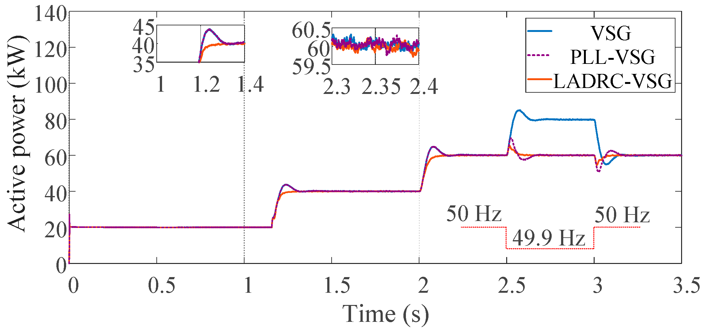
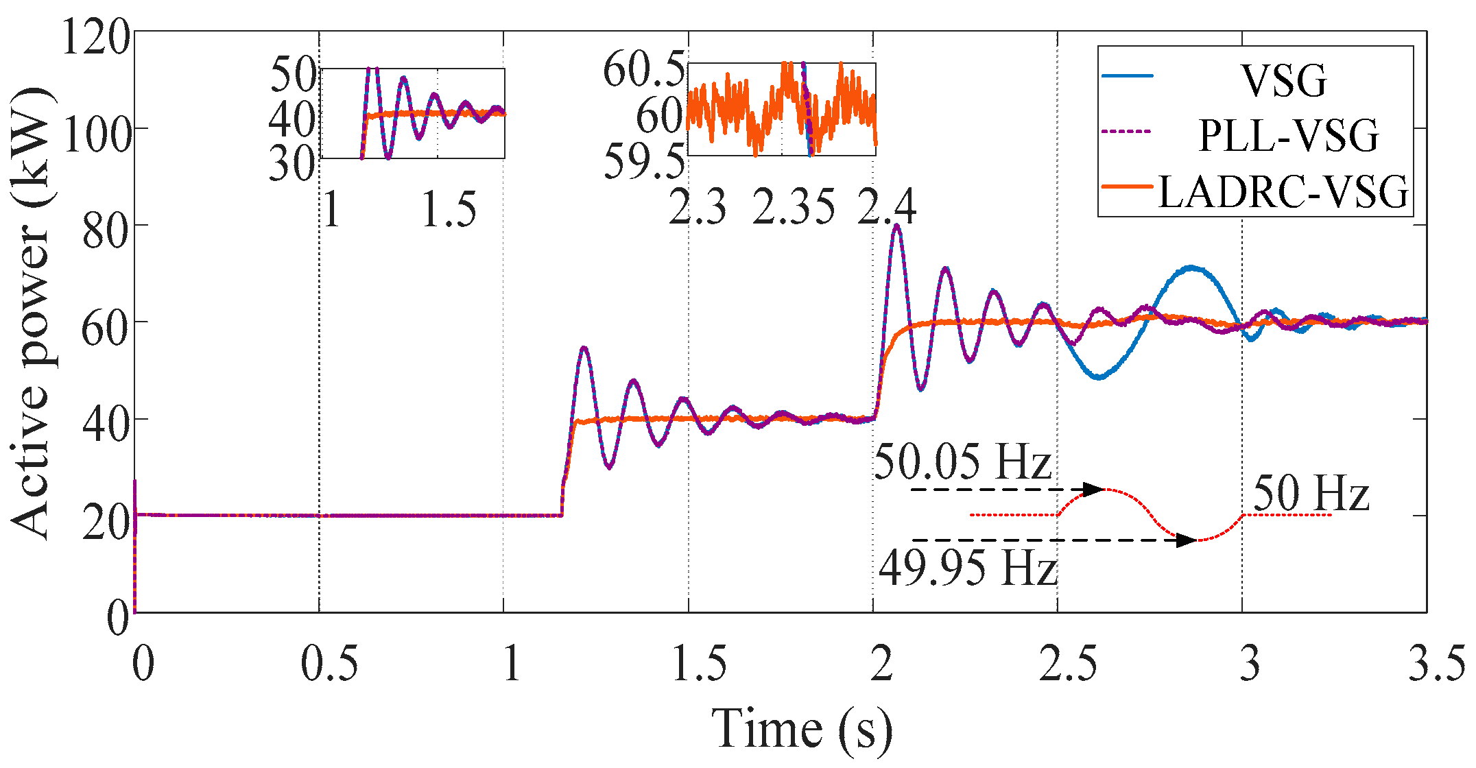
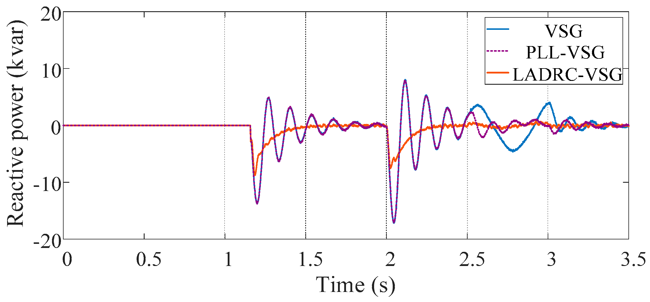
• The proposed control strategy based on LADRC can have VSG output active power to the grid as demanded without overshoot in time compared with the conventional VSG.
• This control strategy enables VSG to transmit power to the grid stably in accordance with the power reference without PLL and it is insensitive to the gird frequency fluctuation.
• The unmodeled parts can be seen as constituent parts of lumped disturbance and the improved VSG has strong robustness to the parameter perturbation and model-plant mismatch.

This article is organized as follows. Section 2 introduces the basic principles of VSG briefly. In Section 3, the drawbacks of transmitting active power to the grid are analyzed by deriving the power transfer function based on the conventional VSG control strategy. Furthermore, the controlling approach for active power of grid-connected VSG is stated based on LADRC, which illustrates the details of modeling. The method for parameter tuning of the designed controller is obtained through frequency domain analyses in Section 4, which contributes to parameter tuning and the performance of the controller. Simulation results are shown in Section 5 to validate the proposed control strategy for power control of grid-connected VSG and Section 6 gives the conclusion of this article with future work proposals.

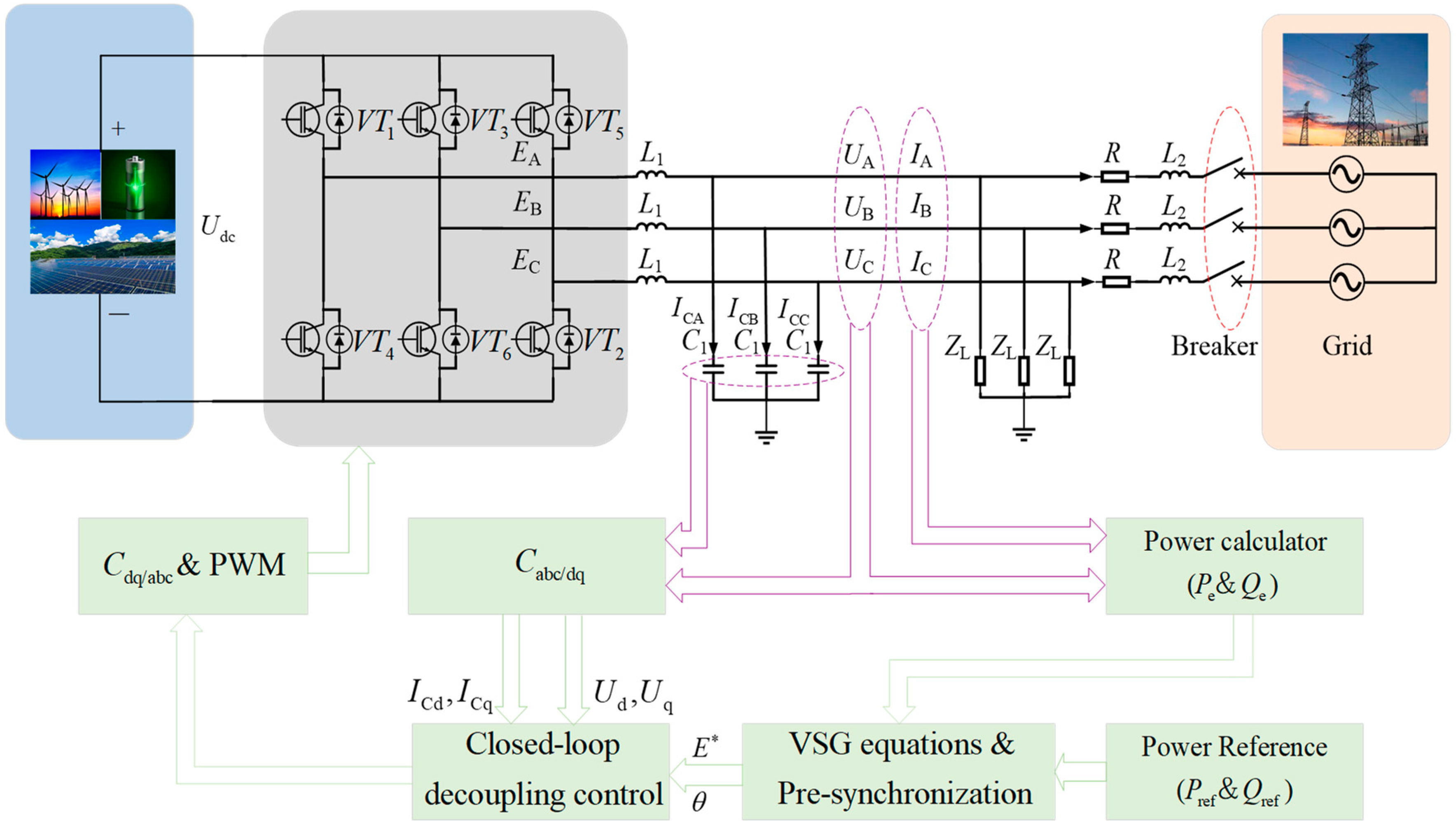
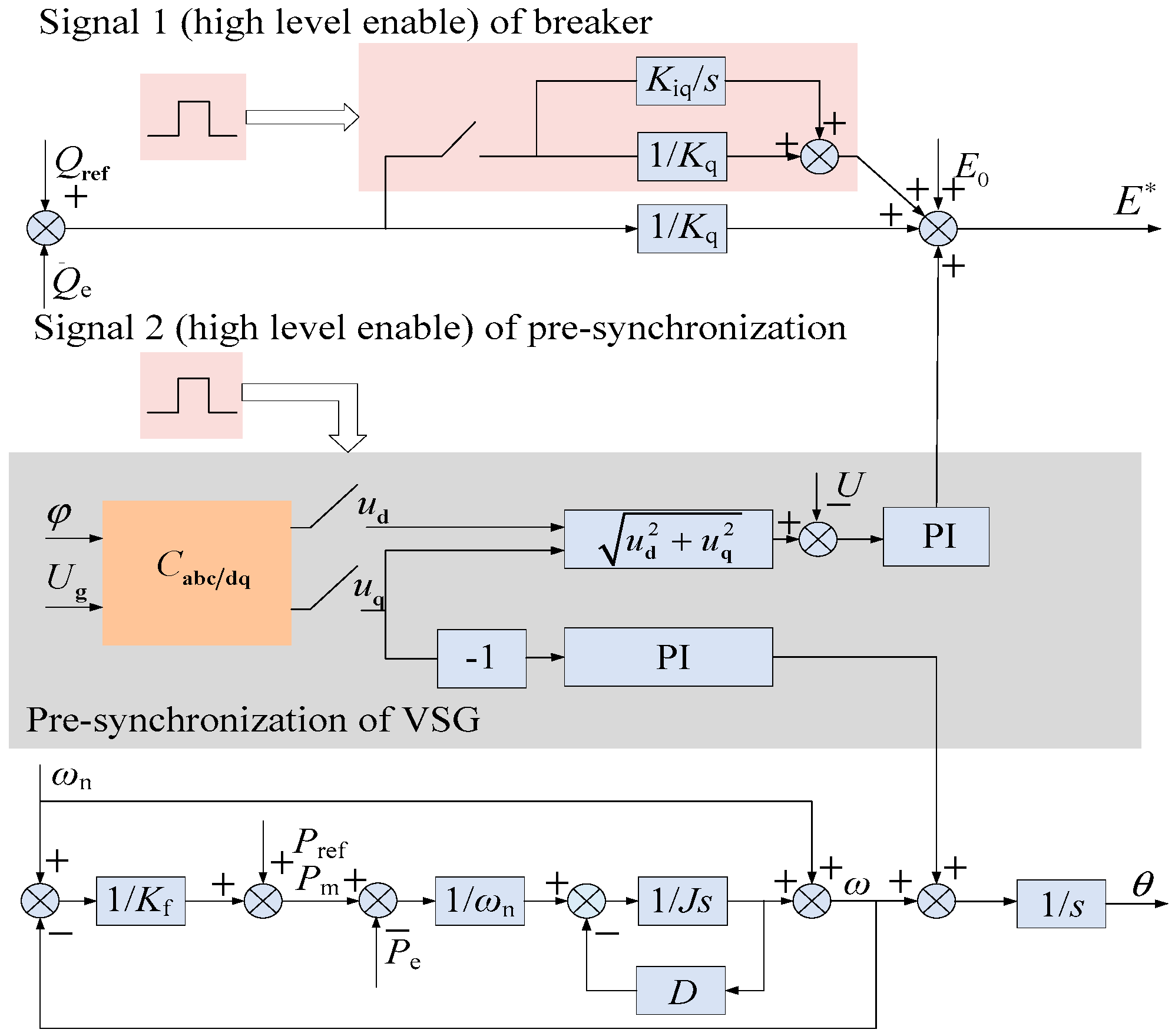
2. Basic Principles of VSG

To emulate the primary frequency modulation characteristic of SG, we assume that the number of pole pairs is one, and the classical equations of the second-order VSG for inverters can be described as

$$P_{\mathrm{m}}=P_{\mathrm{ref}}+\frac{1}{K_{\mathrm{f}}}({\omega }_{\mathrm{n}}-\omega )$$

(1)

$$E^{\ast }=E_0+\frac{1}{K_{\mathrm{q}}}(Q_{\mathrm{ref}}-Q_{\mathrm{e}})$$

(2)

$$\{\begin{array}{l}J\frac{d\omega }{dt}=\frac{P_{\mathrm{m}}-P_{\mathrm{e}}}{\omega }-D(\omega -{\omega }_{\mathrm{n}})\\ \theta ={\displaystyle \int \omega dt}\end{array}$$

(3)

where $P_{\mathrm{m}}$, $P_{\mathrm{ref}}$, $P_{\mathrm{e}}$, $Q_{\mathrm{ref}}$, and $Q_{\mathrm{e}}$ are the mechanical power, the active power reference, the output power, the reactive power reference, and the output reactive power, respectively; $\omega$ and ${\omega }_{\mathrm{n}}$ are denoted as the rotor angular frequency and the rated angular frequency, respectively; $E^{\ast }$ and $E_0$ indicate the voltage reference and the rated peak value of the three-phase voltage, respectively; $K_{\mathrm{f}}$ and $K_{\mathrm{q}}$ are represented as the active power-frequency droop coefficient and the reactive power-voltage droop coefficient, respectively; $J$ is the virtual inertia, $D$ is the damping coefficient, and $\theta$ is the electrical angle. The topology and control structure of the grid-connected VSG are shown in Figure 1.

As shown in Figure 1, $U_{\mathrm{dc}}$ is the constant voltage source containing wind power, solar power, and energy storage system. Here, $L_1$, $L_2$, and $C$ are the filter inductance, the line inductance, and the filter capacitance, respectively; $I_{\mathrm{CA}}$, $I_{\mathrm{CB}}$, and $I_{\mathrm{CC}}$ are the three-phase currents of the capacitance; $E_{\mathrm{A}}$, $E_{\mathrm{B}}$, and $E_{\mathrm{C}}$, and $U_{\mathrm{A}}$, $U_{\mathrm{B}}$, and $U_{\mathrm{C}}$ are introduced to represent the output three-phase voltages of the inverter and the three-phase voltages of the capacitor separately; $I_{\mathrm{Cd}}$ and $I_{\mathrm{Cq}}$, and $U_{\mathrm{d}}$ and $U_{\mathrm{q}}$ are the d-axis and q-axis current of the capacitance, and d-axis and q-axis voltage of the capacitance, respectively; $Z_{\mathrm{L}}$ represents the local loads and the power is denoted as $P_{\mathrm{Local}}$. The breaker is controlled to achieve the switch between the on-grid and off-grid modes of VSG. Besides, the method for pre-synchronization of VSG refers to previous work [25], which proposed the approach of orienting from the q-axis component of grid voltage. The control block is shown in Figure 2, where $U$ is the peak value of the three-phase voltage of VSG, $U_{\mathrm{g}}$ is the three-phase voltage RMS of the grid, and $\phi$ is the initial phase angle of $U_{\mathrm{g}}$. Additionally, to realize better performance of VSG, a proportional-integral controller is introduced into the reactive power control loop when the VSG is connected to the grid. The control block is shown in Figure 2 [17,26,27] and the coefficients of proportionality and integration are $1/K_{\mathrm{q}}$ and $K_{\mathrm{iq}}$, respectively.

3. Control Strategies for VSG

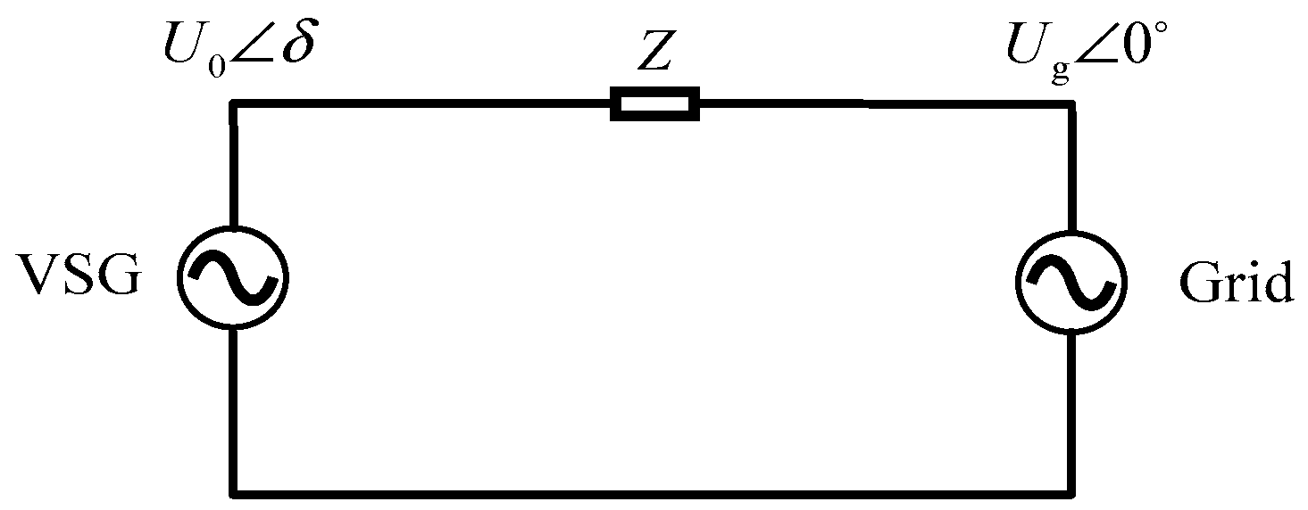
3.1. Performance Analysis of Conventional Grid-Connected VSG

The equivalent topology of the gird-connected VSG and the grid can be illustrated as Figure 3.

As shown in Figure 3, the VSG is equivalent to a SG and it is connected to the grid by three-phase transmission lines, where $Z$ is the line impedance and $Z=R+\mathrm{j}\omega L_2=R+\mathrm{j}X$. Here, $\delta$ is the power angle of VSG and $U_0$ is modeled as the three-phase voltage RMS of VSG. In general, the line is inductive owing to the presence of transformers and filter inductance, thus the apparent power transmitted to the grid by VSG can be given by the following equation [28]:

$$S=3U\stackrel{\ast }{I}=3U\frac{U_0\angle -\delta -U_{\mathrm{g}}\angle 0^{\circ }}{\mathrm{jX}}=P_{\mathrm{e}}+\mathrm{j}{Q}_{\mathrm{e}}=3\frac{U_0{U}_{\mathrm{g}}}{X}\sin \delta +\mathrm{j}(3\frac{U_0{U}_{\mathrm{g}}}{X}\cos \delta -3\frac{U_{\mathrm{g}}{}^2}{X})$$

(4)

where $\delta$ is generally seen as a small value, $\sin \delta \approx \delta$. Then, $P_{\mathrm{e}}$ in Equation (4) can be linearized as [12]:

$$P_{\mathrm{e}}=\frac{3U_0{U}_{\mathrm{g}}\delta }{X}$$

(5)

Now, we let $\omega ={\omega }_{\mathrm{n}}$ when calculating the torque deviation, and we also have the switching of electronic devices, the fine adjustment process of voltage, and the current double closed loop omitted. Combining Equations (1)–(3) with (5), the equivalent active power control block diagram of the grid-connected VSG can be obtained as Figure 4.

Here, ${\omega }_{\mathrm{g}}$ is the real-time angular grid frequency and $C=3\frac{U_0{U}_g}{X}$. Letting $\mathsf{\Delta }{\omega }_{\mathrm{ng}}={\omega }_{\mathrm{n}}-{\omega }_{\mathrm{g}}$, therefore, the output active power can be modeled as:

$$P_{\mathrm{e}}(s)=\frac{C{K}_{\mathrm{f}}}{K_{\mathrm{f}}J{\omega }_{\mathrm{n}}{s}^2+(K_{\mathrm{f}}D{\omega }_{\mathrm{n}}+1)s+C{K}_{\mathrm{f}}}{P}_{\mathrm{ref}}(s)+\frac{C(K_{\mathrm{f}}J{\omega }_{\mathrm{n}}s+K_{\mathrm{f}}D{\omega }_{\mathrm{n}}+1)}{K_{\mathrm{f}}J{\omega }_{\mathrm{n}}{s}^2+(K_{\mathrm{f}}D{\omega }_{\mathrm{n}}+1)s+C{K}_{\mathrm{f}}}\mathsf{\Delta }{\omega }_{\mathrm{ng}}(s)$$

(6)

We suppose that the grid frequency does not fluctuate, i.e., ${\omega }_{\mathrm{n}}={\omega }_{\mathrm{g}}$. Then, Equation (6) can be transformed into:

$$P_{\mathrm{e}}(s)=\frac{C{K}_{\mathrm{f}}}{K_{\mathrm{f}}J{\omega }_{\mathrm{n}}{s}^2+(K_{\mathrm{f}}D{\omega }_{\mathrm{n}}+1)s+C{K}_{\mathrm{f}}}{P}_{\mathrm{ref}}(s)$$

(7)

The coefficients of the characteristic equation in Equation (7) are all greater than zero, and the system is stable. Further, the damping ratio of Equation (7) can be obtained as:

$${\xi }_1=\frac{D}{2}\sqrt{\frac{{\omega }_{\mathrm{n}}}{JC}}+\frac{1}{2K_{\mathrm{f}}}\sqrt{\frac{1}{J{\omega }_{\mathrm{n}}C}}$$

(8)

It is clear that ${\xi }_1$ increases, the overshoot decreases, and the system responds more slowly with the increase of $D$. If $J$ decreases, the overshoot will increase, and thus the response speed will accelerate. There exists a contradiction to be solved between the rapid response and the overshoot of output power.

The final value theorem [29] can be applied to Equation (7), and the steady-state power output to the grid can be calculated as $P_{\mathrm{e}}=P_{\mathrm{ref}}$. However, in reality, the grid frequency is always fluctuating, and it is difficult for VSG to operate stably at the rated frequency. Therefore,

$$\frac{P_{\mathrm{e}}(s)}{\Delta {\omega }_{\mathrm{ng}}(s)}=\frac{C(K_{\mathrm{f}}J{\omega }_{\mathrm{n}}s+K_{\mathrm{f}}D{\omega }_{\mathrm{n}}+1)}{K_{\mathrm{f}}J{\omega }_{\mathrm{n}}{s}^2+(K_{\mathrm{f}}D{\omega }_{\mathrm{n}}+1)s+C{K}_{\mathrm{f}}}$$

(9)

Supposing $\mathsf{\Delta }{\omega }_{\mathrm{ng}}$ is the unit step signal, the steady-state power deviation can be deduced as

$$\Delta P_{\mathrm{e}}=D{\omega }_{\mathrm{n}}+\frac{1}{K_{\mathrm{f}}}$$

(10)

It can be perceived from Equation (10) that there is a negative correlation between $K_{\mathrm{f}}$ and $\Delta P_{\mathrm{e}}$, and a positive correlation between $D$ and $\Delta P_{\mathrm{e}}$ separately. However, under the condition that ${\omega }_{\mathrm{n}}\ne {\omega }_{\mathrm{g}}$, the presence of the difference between $P_{\mathrm{e}}$ and $P_{\mathrm{ref}}$ cannot be eliminated if $K_{\mathrm{f}}$ and $D$ are changed to reduce the deviation. The overload coefficient of the inverter shall not exceed 1.5 in practice generally, and if $\mathsf{\Delta }{\omega }_{\mathrm{ng}}$ is too large, the actual output power of the VSG may exceed the maximum permissible power of the inverter. As one example, the extreme operation of the VSG may trigger its overcurrent protection, which will cause it to detach from the grid; as another example, if VSG is not disconnected from the grid, the long period of overloading can shorten its life. Hence, a strategy that enables VSG output power according to the reference is needed if ${\omega }_{\mathrm{g}}$ fluctuates or in some other extreme circumstances.

3.2. Control Strategy for Power of Grid-Connected VSG Based on LADRC

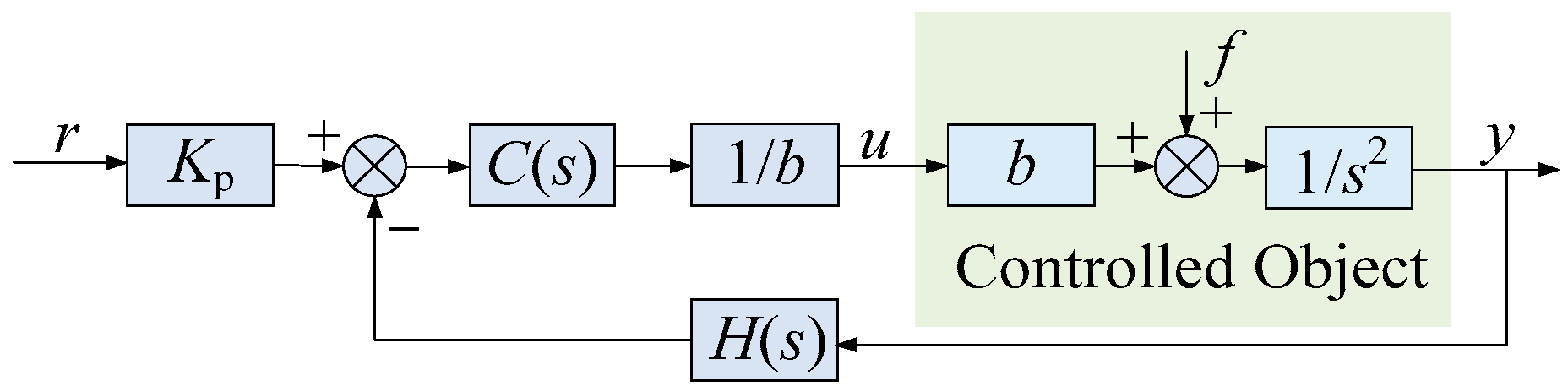
3.2.1. Principles of the Second-Order LADRC

It can be observed that the controlled object (6) is a second-order model, thus we design a second-order LADRC power controller to solve the above problems accordingly. The second-order LADRC controller consists of a linear extended state observer (LESO) and linear state error feedback (LSEF). The advantage of LADRC is that LESO can regard the lumped disturbance as one of the variable states of the system to be observed. Its basic control structure is shown in Figure 5 [30], where $r$ is the reference and $y$ is the output of the controlled object. The estimation for the output of the controlled object, the derivative value of the output, and the lumped disturbance are denoted as $z_1$, $z_2$, and $z_3$, respectively. Additionally, $b$ is the gain of the controlled object, $u$ is the compensated control value, $e$ is the difference between $y$ and $z_1$; $l_1$, $l_2$, and $l_3$ are the different error feedback gain factors in LESO.

Here, $f$ is denoted as the lumped disturbance, and the time-domain expression of the controlled object can be written as:

$$\ddot{y}=f(y,\dot{y},w,t)+bu$$

(11)

The model of LESO can be designed as:

$$\{\begin{array}{l}e=y-z_1\\ {\dot{z}}_1=z_2+l_{1}e\\ {\dot{z}}_2=z_3+l_{2}e+bu\\ {\dot{z}}_3=l_{3}e\end{array}$$

(12)

Noticing Equation (11), the expression of the controlled object can be written in state space form as:

$$\left[\begin{array}{l}{\dot{x}}_1\\ {\dot{x}}_2\\ {\dot{x}}_3\end{array}\right]=\left[\begin{array}{ccc}0& 1& 0\\ 0& 0& 1\\ 0& 0& 0\end{array}\right]\left[\begin{array}{c}{x}_1\\ x_2\\ x_3\end{array}\right]+\left[\begin{array}{c}0\\ b\\ 0\end{array}\right]u+\left[\begin{array}{l}0\\ 0\\ 1\end{array}\right]f$$

(13)

$$y=\left[\begin{array}{ccc}1& 0& 0\end{array}\right]\left[\begin{array}{l}y\\ \dot{y}\\ f\end{array}\right]$$

(14)

Combining Equation (12) with Equations (13) and (14), the expression of the three-order LESO can be deduced as:

$$\left[\begin{array}{l}{\dot{z}}_1\\ {\dot{z}}_2\\ {\dot{z}}_3\end{array}\right]=\left[\begin{array}{ccc}-l_1& 1& 0\\ -l_2& 0& 1\\ -l_3& 0& 0\end{array}\right]\left[\begin{array}{c}{z}_1\\ z_2\\ z_3\end{array}\right]+\left[\begin{array}{cc}\begin{array}{l}0\\ b\\ 0\end{array}& \begin{array}{l}{l}_1\\ l_2\\ l_3\end{array}\end{array}\right]\left[\begin{array}{l}u\\ y\end{array}\right]$$

(15)

Then, taking the Laplace transformation of Equation (15), we have:

$$Z\left(s\right)=\frac{1}{s^3+l_1{s}^2+l_{2}s+l_3}\left[\begin{array}{cc}bs& l_1{s}^2+l_{2}s+l_3\\ b{s}^2+b{l}_{1}s& l_2{s}^2+l_{3}s\\ -b{l}_3& l_3{s}^2\end{array}\right]\left[\begin{array}{c}U(s)\\ Y(s)\end{array}\right]$$

(16)

Based on the estimated states, LSEF can be designed as:

$$u=\frac{K_{\mathrm{p}}(r-z_1)-K_{\mathrm{d}}{z}_2-z_3}{b}$$

(17)

where $K_{\mathrm{p}}$ and $K_{\mathrm{d}}$ are the gains of LSEF. According to Equations (16) and (17), it can be seen that:

$$U(s)=\frac{1}{b}[K_{p}R(s)C(s)-Y(s)H(s)C(s)]$$

(18)

where

$$C(s)=\frac{s^3+l_1{s}^2+l_{2}s+l_3}{s^3+(l_1+K_{\mathrm{d}})s^2+(l_1{K}_{\mathrm{d}}+l_2+K_{\mathrm{p}})s}$$

(19)

$$H(s)=\frac{(K_{\mathrm{p}}{l}_1+k_{\mathrm{d}}{l}_2+l_3)s^2+(K_{\mathrm{p}}{l}_2+k_{\mathrm{d}}{l}_3)s+K_{\mathrm{P}}{l}_3}{s^3+l_1{s}^2+l_{2}s+l_3}$$

(20)

Combining Equation (11) with Equations (18)–(20), the simplified control structure can be drawn in Figure 6.

As shown in Figure 6, the control structure of active power does not become complicated, and it can be deduced as the classical feedback control structure where the disturbance is considered. Based on the estimations of output and disturbance, LSEF can compensate for the controlled variable in feedback, which will quickly make the output track the reference without offset. If the observations are reliable, then $z_1\to y$, $z_2\to \dot{y}$, $z_3\to f$. According to Equations (12) and (17), the differential equation can be derived as:

$$\ddot{y}=-K_{\mathrm{d}}\dot{y}-K_{\mathrm{p}}y+K_{\mathrm{p}}r$$

(21)

The closed-loop transfer function of the system can be deduced by the classical control theory as:

$$\frac{Y(s)}{R(s)}=\frac{K_{\mathrm{p}}}{s^2+K_{\mathrm{d}}s+K_{\mathrm{p}}}$$

(22)

A previous study [24] proposed a parameter tuning method for LADRC based on the bandwidths, which can track the reference without overshoot in a timely manner. Therefore, $l_1$, $l_2$, and $l_3$, and $K_{\mathrm{p}}$ and $K_{\mathrm{d}}$ are relevant to the bandwidth of LESO and that of LSEF, which are noted as ${\omega }_{\mathrm{o}}$ and ${\omega }_{\mathrm{c}}$, respectively. The tuning details are given by:

$$\{\begin{array}{l}{l}_1=3{\omega }_{\mathrm{o}}, l_2=3{\omega }_{\mathrm{o}}^2, l_3={\omega }_{\mathrm{o}}^3\\ K_{\mathrm{d}}=2{\omega }_{\mathrm{c}}, K_{\mathrm{p}}={\omega }_{\mathrm{c}}^2\end{array}$$

(23)

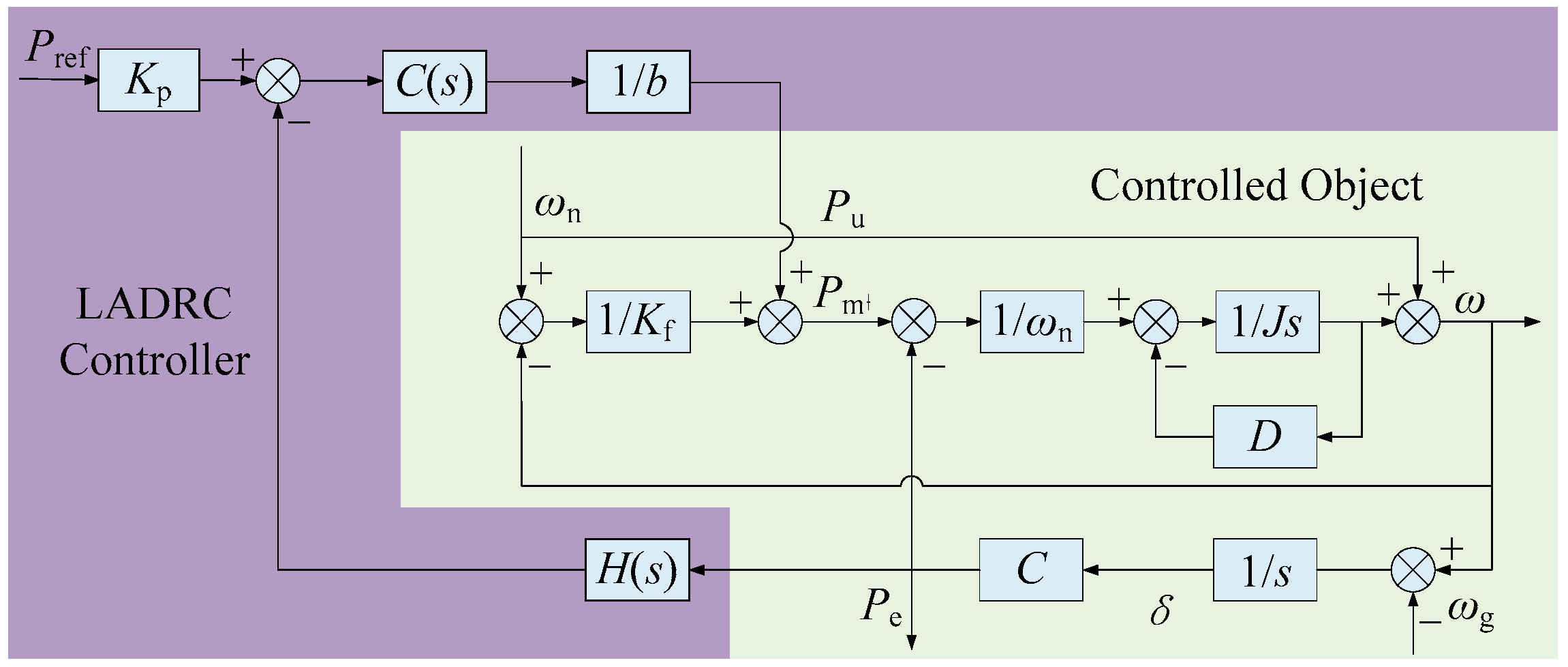
3.2.2. Control Strategy for Active Power of VSG Based on LADRC

According to Equation (11), Equation (6) can be derived in the time domain as:

$$\frac{{\mathrm{d}}^2{P}_{\mathrm{e}}}{\mathrm{d}{t}^2}=-\frac{(K_{\mathrm{f}}D{\omega }_{\mathrm{n}}+1)}{K_{\mathrm{f}}J{\omega }_{\mathrm{n}}}\frac{d{P}_{\mathrm{e}}}{\mathrm{d}t}-\frac{C{P}_{\mathrm{e}}}{J{\omega }_{\mathrm{n}}}+C\frac{d\mathsf{\Delta }{\omega }_{\mathrm{ng}}}{\mathrm{d}t}+\frac{C(K_{\mathrm{f}}D{\omega }_{\mathrm{n}}+1)}{K_{\mathrm{f}}J{\omega }_{\mathrm{n}}}\mathsf{\Delta }{\omega }_{\mathrm{ng}}+\frac{C}{J{\omega }_{\mathrm{n}}}{P}_{\mathrm{ref}}=f+\frac{C}{J{\omega }_{\mathrm{n}}}{P}_{\mathrm{ref}}=f+bu$$

(24)

Thus, the equivalent control structure of power based on LADRC can be obtained according to Section 3.1 as Figure 7.

Here, $P_{\mathrm{u}}$ is the compensated control value and the transfer function of power can be stated as:

$$P_{\mathrm{e}}(s)=\frac{N(s)}{Q\left(s\right)}{P}_{\mathrm{ref}}(s)+\frac{M(s)}{Q\left(s\right)}[{\omega }_{\mathrm{n}}(s)-{\omega }_{\mathrm{g}}(s)]=\frac{N(s)}{Q\left(s\right)}{P}_{\mathrm{ref}}(s)+\frac{M(s)}{Q\left(s\right)}\Delta {\omega }_{\mathrm{ng}}(s)$$

(25)

where

$$N(s)=C{K}_{\mathrm{f}}{\omega }_{\mathrm{c}}^2(s^3+3{\omega }_{\mathrm{o}}{s}^2+3{\omega }_{\mathrm{o}}^{2}s+{\omega }_{\mathrm{o}}^3)$$

(26)

$$\begin{array}{c}M(s)=bC{K}_{\mathrm{f}}J{\omega }_{\mathrm{n}}{s}^4+bC[K_{\mathrm{f}}J{\omega }_{\mathrm{n}}(3{\omega }_{\mathrm{o}}+2{\omega }_{\mathrm{c}})+K_{\mathrm{f}}D{\omega }_{\mathrm{n}}+1]s^3+bC[K_{\mathrm{f}}J{\omega }_{\mathrm{n}}(6{\omega }_{\mathrm{o}}{\omega }_{\mathrm{c}}+3{\omega }_{\mathrm{o}}^2+{\omega }_{\mathrm{c}}^2)+\\ (K_{\mathrm{f}}D{\omega }_{\mathrm{n}}+1)(3{\omega }_{\mathrm{o}}+2{\omega }_{\mathrm{c}})]s^2+bC(K_{\mathrm{f}}D{\omega }_{\mathrm{n}}+1)(6{\omega }_{\mathrm{o}}{\omega }_{\mathrm{c}}+3{\omega }_{\mathrm{o}}^2+{\omega }_{\mathrm{c}}^2)s\end{array}$$

(27)

$$Q(s)=q_1{s}^5+q_2{s}^4+q_3{s}^3+q_4{s}^2+q_{5}s+q_6$$

(28)

In Equation (28), $q_1–q_6$ are the constant values obtained by deducing the transfer function in Figure 7. It is obvious that the transient process of power is influenced by two factors directly, which are the power reference and $\Delta {\omega }_{\mathrm{ng}}$, respectively. Besides, according to Equations (27) and (28), the steady-state power output has no tracking offset if $\Delta {\omega }_{\mathrm{ng}}$ is a step change value. It indicates the ability to suppress the disturbance under the LADRC control strategy for VSG. In addition, it can be further seen in Equation (24) that $\Delta {\omega }_{\mathrm{ng}}$ is not the only part of the lumped disturbance. The influence of the difference between power reference and the output active power and its differential value, the influence of the difference of angular frequency reference, and the grid angular frequency and its differential value are all taken as the components of the lumped disturbance. Furthermore, some other factors that are unmodeled, which bring deviation to the active power, are all regarded as the components of lump disturbance and compensated. If the lumped disturbance can be observed and compensated precisely, an integrator series structure can be obtained. Therefore, the output can track the reference without overshoot and deviation, even though the plant is not accurate enough. This further shows the advantage that LADRC does not rely on the precise model of the controlled object.

4. Parameters Tuning for Controller

4.1. Nominal Performance Concerning

The stability of the control system is the premise for LADRC to achieve great performance in the power control of the grid-connected VSG. The stability margin of LADRC should be determined and the controller parameters need to be tuned first. According to previous work [24], there are three parameters remaining to be determined: $b$, ${\omega }_{\mathrm{o}}$, and ${\omega }_{\mathrm{c}}$. Now, we combine Equation (24) with

Table 1. Key parameters of the system.

Parameter	Symbol	Value	Parameter	Symbol	Value
$U_{\mathrm{g}}$	$\mathrm{V}$	220	$U_{\mathrm{dc}}$	$\mathrm{V}$	800
$D$	$\mathrm{N}\cdot \mathrm{m}\cdot {\mathrm{rad}}^{-1}$	100	$J$	$\mathrm{kg}\cdot {\mathrm{m}}^2$	0.8
$K_{\mathrm{q}}$	—	3330	$L_1$	$\mathrm{mH}$	0.6
$K_{\mathrm{iq}}$	—	0.005	$L_2$	$\mathrm{mH}$	0.404
$K_{\mathrm{f}}$	—	0.0628	$C_1$	$\mu \mathrm{F}$	1500
$R$	$\mathsf{\Omega }$	0.1	${\omega }_{\mathrm{n}}$	${\mathrm{rad}}^{-1}\cdot \mathrm{s}$	314.16

, and $b$ can be calculated as:

$$b=\frac{C}{J{\omega }_{\mathrm{n}}}=4597$$

(29)

In order to clarify the relationship between the parameters when the system is stable, the characteristic equation of the closed loop transfer function can be obtained as:

$$q_1{s}^5+q_2{s}^4+q_3{s}^3+q_4{s}^2+q_{5}s+q_6=0$$

(30)

where

$$q_1=b{K}_{\mathrm{f}}J{\omega }_{\mathrm{n}}$$

(31)

$$q_2=b{K}_{\mathrm{f}}J{\omega }_{\mathrm{n}}(3{\omega }_{\mathrm{o}}+2{\omega }_{\mathrm{c}})+b(K_{\mathrm{f}}D{\omega }_{\mathrm{n}}+1)$$

(32)

$$q_3=b{K}_{\mathrm{f}}J{\omega }_{\mathrm{n}}(6{\omega }_{\mathrm{o}}{\omega }_{\mathrm{c}}+{\omega }_{\mathrm{c}}^2+3{\omega }_{\mathrm{o}}^2)+b(K_{\mathrm{f}}D{\omega }_{\mathrm{n}}+1)(3{\omega }_{\mathrm{o}}+2{\omega }_{\mathrm{c}})+bC{K}_{\mathrm{f}}$$

(33)

$$q_4=b(K_{\mathrm{f}}D{\omega }_{\mathrm{n}}+1)(6{\omega }_{\mathrm{o}}{\omega }_{\mathrm{c}}+{\omega }_{\mathrm{c}}^2+3{\omega }_{\mathrm{o}}^2)+C{K}_{\mathrm{f}}({\omega }_{\mathrm{o}}^3+3{\omega }_{\mathrm{o}}{\omega }_{\mathrm{c}}^2+6{\omega }_{\mathrm{c}}{\omega }_{\mathrm{o}}^2+3b{\omega }_{\mathrm{o}}+2b{\omega }_{\mathrm{c}})$$

(34)

$$q_5=C{K}_{\mathrm{f}}(6b{\omega }_{\mathrm{o}}{\omega }_{\mathrm{c}}+3b{\omega }_{\mathrm{o}}^2+b{\omega }_{\mathrm{c}}^2+3{\omega }_{\mathrm{o}}^2{\omega }_{\mathrm{c}}^2+2{\omega }_{\mathrm{c}}{\omega }_{\mathrm{o}}^3)$$

(35)

$$q_6=C{K}_{\mathrm{f}}{\omega }_{\mathrm{c}}^2{\omega }_{\mathrm{o}}^3$$

(36)

The Lienard–Chipard criterion can be applied to judge whether the system is stable or not. The necessary and sufficient condition for stability is that the coefficients of the characteristic equation and each odd (or even) order Hurwitz determinant are greater than zero separately. It is noticeable that the coefficients of the characteristic equation are all greater than zero. Therefore, the necessary and sufficient condition for the stability of the system can be simplified as [31]:

$${\Delta }_5=(q_2{q}_3-q_1{q}_4)(q_4{q}_5-q_3{q}_6)-{(q_2{q}_5-q_1{q}_6)}^2>0$$

(37)

Thus, preliminarily, the relationship between ${\omega }_{\mathrm{o}}$ and ${\omega }_{\mathrm{c}}$ can be determined when the system is stable, according to the constraint in Equation (37). However, the Lienard–Chipard criterion cannot reflect the degree of stability. To obtain the reliable parameters of LADRC further, it is necessary to analyze the influence of different parameters on the performance of the LADRC controller. Combined with the above analyses, the initial values are chosen as ${\omega }_{\mathrm{o}0}=300$ and ${\omega }_{\mathrm{c}0}=300$. The influence on the performance of the controller will be discussed with the changes of ${\omega }_{\mathrm{o}}$ and ${\omega }_{\mathrm{c}}$.

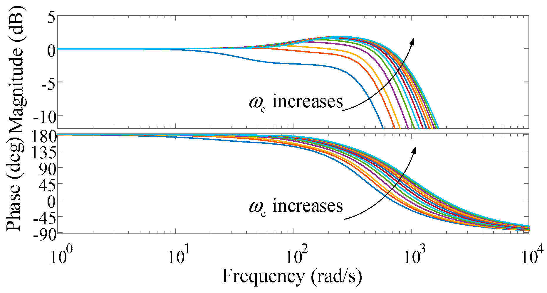
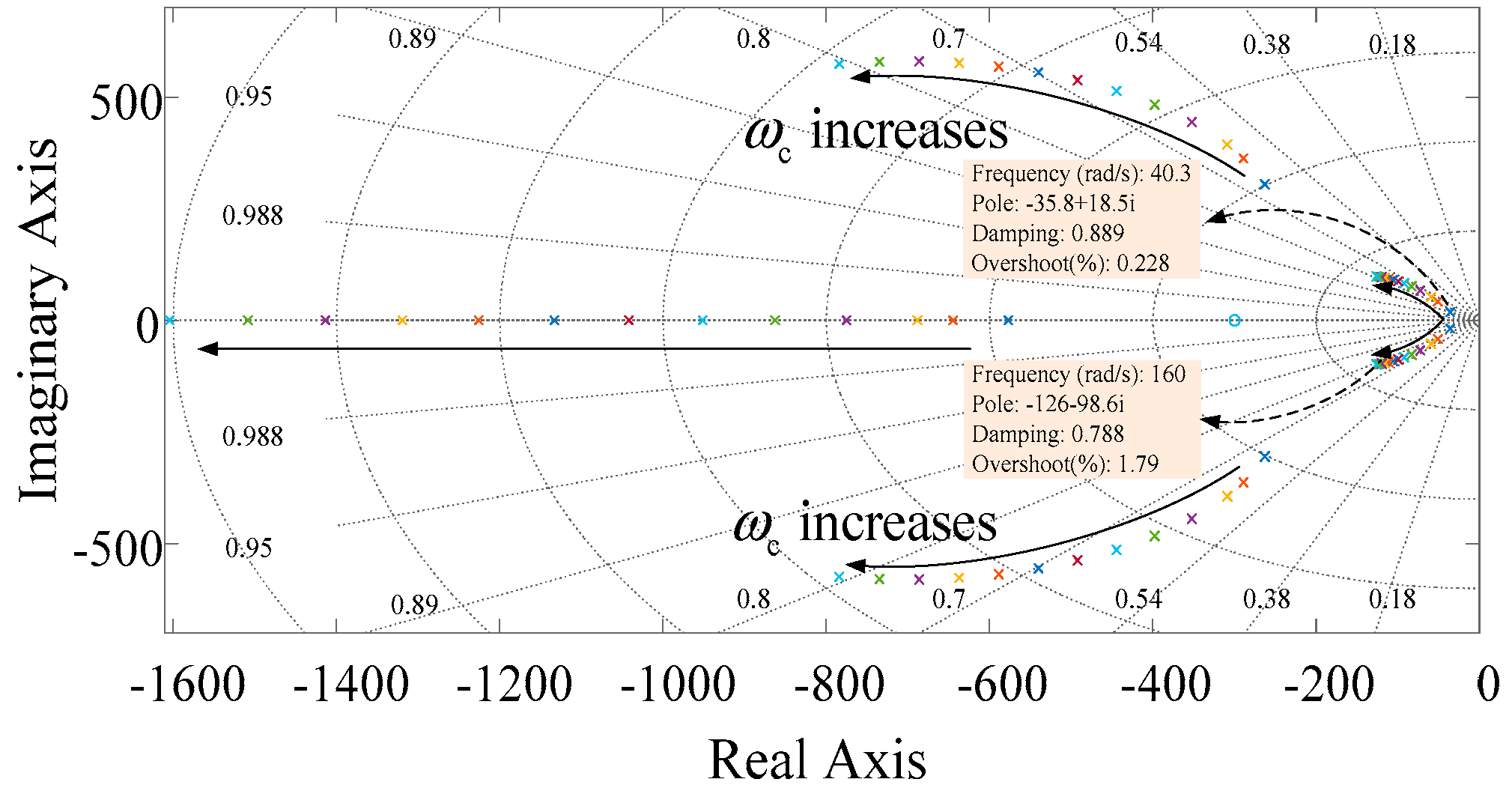
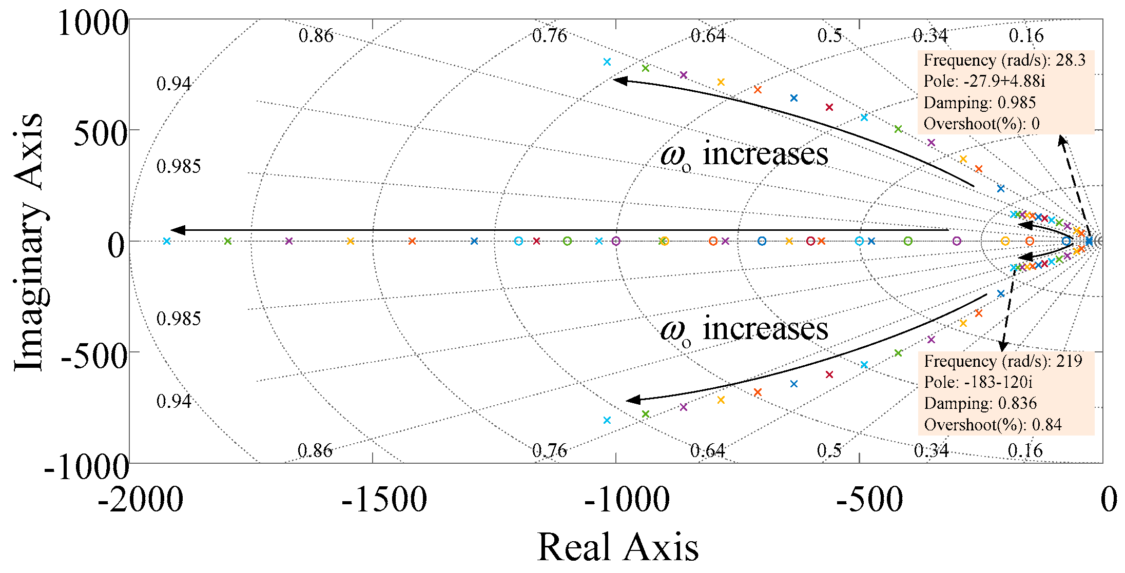
4.1.1. Parameter ${\omega }_{\mathrm{c}}$ Increases When ${\omega }_{\mathrm{o}}$ Remains Unchanged

The parameter ${\omega }_{\mathrm{c}}$ increases from $0.25{\omega }_{\mathrm{c}0}$ to $4{\omega }_{\mathrm{c}0}$ gradually. The pole-zero map of the transfer function from $P_{\mathrm{ref}}$ to $P_{\mathrm{e}}$ and the Bode diagram of the transfer function from $\Delta {\omega }_{\mathrm{ng}}$ to $P_{\mathrm{e}}$ are given in Figure 8 and Figure 9, respectively.

As we can see in Figure 8, the closed-loop poles move away from the imaginary axis gradually and the response of the output accelerates with the increase of ${\omega }_{\mathrm{c}}$. However, the angle between the dominant poles and the negative real axis increases first and then decreases, which can be perceived as the damping of the system experiencing the process of first decreasing and then increasing. When ${\omega }_{\mathrm{c}}$ is determined as the smallest value of $0.25{\omega }_{\mathrm{c}0}$, the system has the largest damping value, which means that a larger value of ${\omega }_{\mathrm{c}}$ may cause overshoot of the power output. In addition, it can be perceived that ${\omega }_{\mathrm{c}}$ does not affect the position of the zero point. According to Appendix A, if the value of ${\omega }_{\mathrm{c}}$ is too large, the high-frequency measurement noise would be amplified more obviously, and this will deteriorate the control performance. In Figure 9, with the increase of the frequency from the band of 1 $\mathrm{rad}/\mathrm{s}$ to 100 $\mathrm{rad}/\mathrm{s}$, the ability of anti-disturbance will be reduced. Besides, if ${\omega }_{\mathrm{c}}$ increases, the gain of $\Delta {\omega }_{\mathrm{ng}}$ will decrease, and the output is less sensitive to the low frequency disturbance. This is to say, if the disturbance rejecting ability needs to be enhanced, we can increase ${\omega }_{\mathrm{c}}$ on the premise that the measurement noise is bearable for the system.

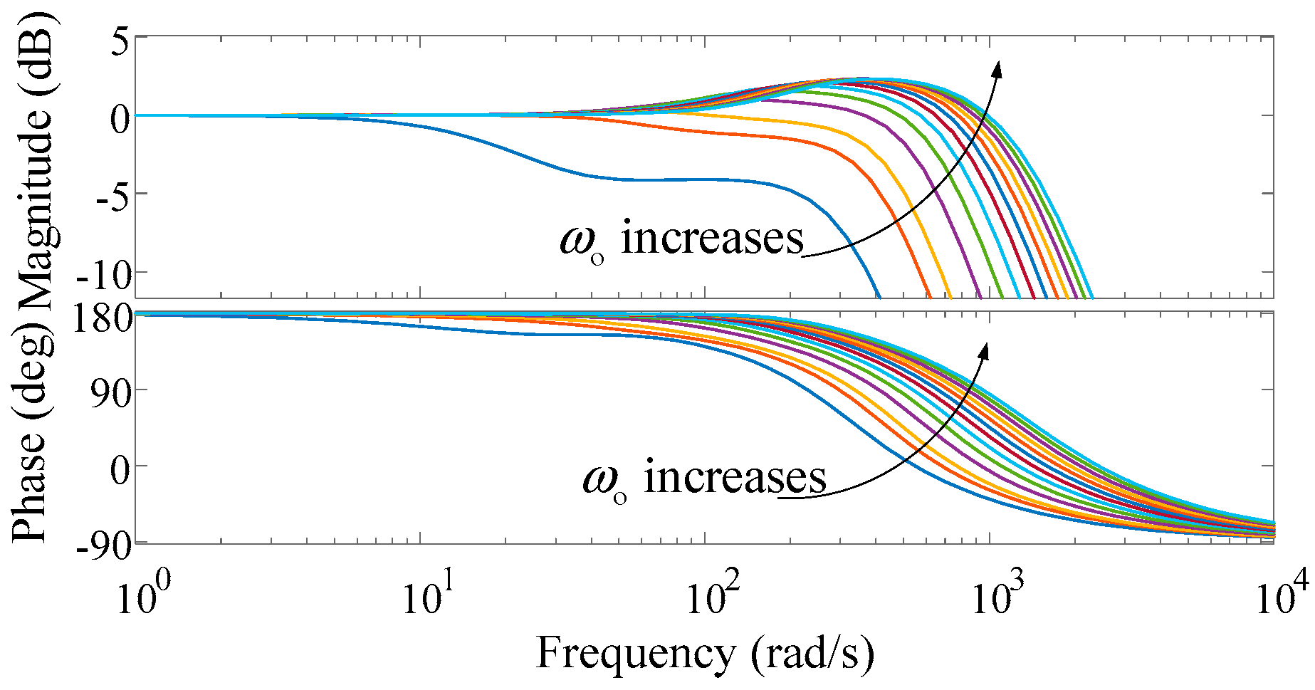
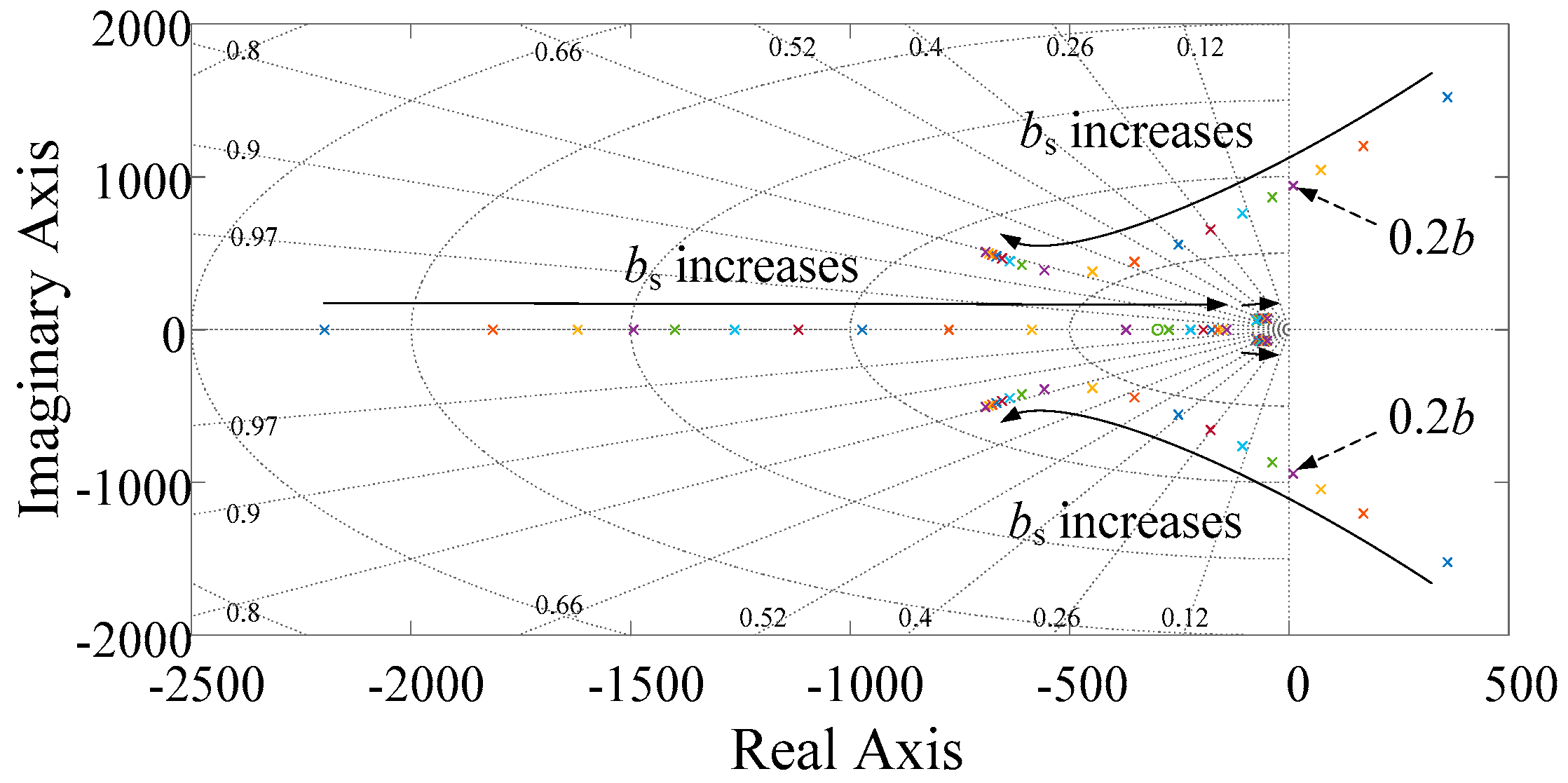
4.1.2. Parameter ${\omega }_{\mathrm{o}}$ Increases When ${\omega }_{\mathrm{c}}$ Remains Unchanged

The parameter ${\omega }_{\mathrm{o}}$ increases from $0.25{\omega }_{\mathrm{o}0}$ to $4{\omega }_{\mathrm{o}0}$ gradually. The pole-zero map of the transfer function from $P_{\mathrm{ref}}$ to $P_{\mathrm{e}}$ and the Bode diagram of the transfer function from $\Delta {\omega }_{\mathrm{ng}}$ to $P_{\mathrm{e}}$ are given in Figure 10 and Figure 11, respectively.

It can be seen from Figure 10 that the closed-loop poles move away from the imaginary axis gradually with the increase of ${\omega }_{\mathrm{o}}$, which is similar to Figure 8. The increase of ${\omega }_{\mathrm{o}}$ can also accelerate the response speed of the system, which can track the power reference more rapidly. When ${\omega }_{\mathrm{o}}$ is small, the closed-loop zero points and dominant poles form dipoles and the equivalent order of the system can be reduced to some extent. However, with the increase of ${\omega }_{\mathrm{o}}$, the dipoles no longer exist. Besides, the ability of rejecting disturbance increases when ${\omega }_{\mathrm{o}}$ increases, as shown in Figure 11.

At the same time, as introduced in Appendix A, the measurement noise would be amplified more evidently with the increase of ${\omega }_{\mathrm{o}}$. Moreover, depending on the combinations of Figure 8 and Figure 10, a phenomenon can be seen showing that ${\omega }_{\mathrm{o}}$ has a deeper influence on the positions of dominant poles and the dynamic characteristics of the system when the two parameters have the same change. When the frequency of disturbance is 1 rad/s, the range of the gain of $\Delta {\omega }_{\mathrm{ng}}$, which is a part of the lumped disturbance, is from 23.2 dB to 51.8 dB and from 15.6 dB to 59.4 dB in Figure 9 and Figure 11, respectively. When the values of the two parameters have the same change, the change of ${\omega }_{\mathrm{o}}$ has a stronger influence on the ability to suppress the disturbance than the change of ${\omega }_{\mathrm{c}}$.

Additionally, $b_{\mathrm{s}}$ is the set value of $b$ in the controller. In this article, the value of $b$ can be calculated out. Supposing the condition that the gain of the model is hard to obtain, we can draw the pole-zero map of $\frac{N\left(s\right)}{Q\left(s\right)}$ and the Bode diagram of $\frac{M\left(s\right)}{Q\left(s\right)}$ as Figure 12 and Figure 13, respectively. Therefore, the influences of different values of $b_{\mathrm{s}}$ on the control performance can be analyzed, letting ${\omega }_{\mathrm{o}0}={\omega }_{\mathrm{c}0}=300$ and $b_{\mathrm{s}}$ change from $0.05b$ to $3b$.

It can be seen in Figure 12 that when $b_{\mathrm{s}}$ is smaller than $0.2b$, the system will collapse. Further, if $b_{\mathrm{s}}$ is determined as a value greater than approximately $0.2b$, the system will be stable. Moreover, it can be seen in Figure 13 that when $b_{\mathrm{s}}$ is a relatively large value, the gain of disturbance will increase. In other words, there is a tradeoff between the stability of the system and the ability to suppress the disturbance when the gain of the controlled object is hard to obtain. We need to tune $b_{\mathrm{s}}$ from a large value to a small value for stability consideration. When the system is stable, we can decrease the value of $b_{\mathrm{s}}$ concerning disturbance-rejection.

Above all, the tuning method for the parameters can be summarized as follows:

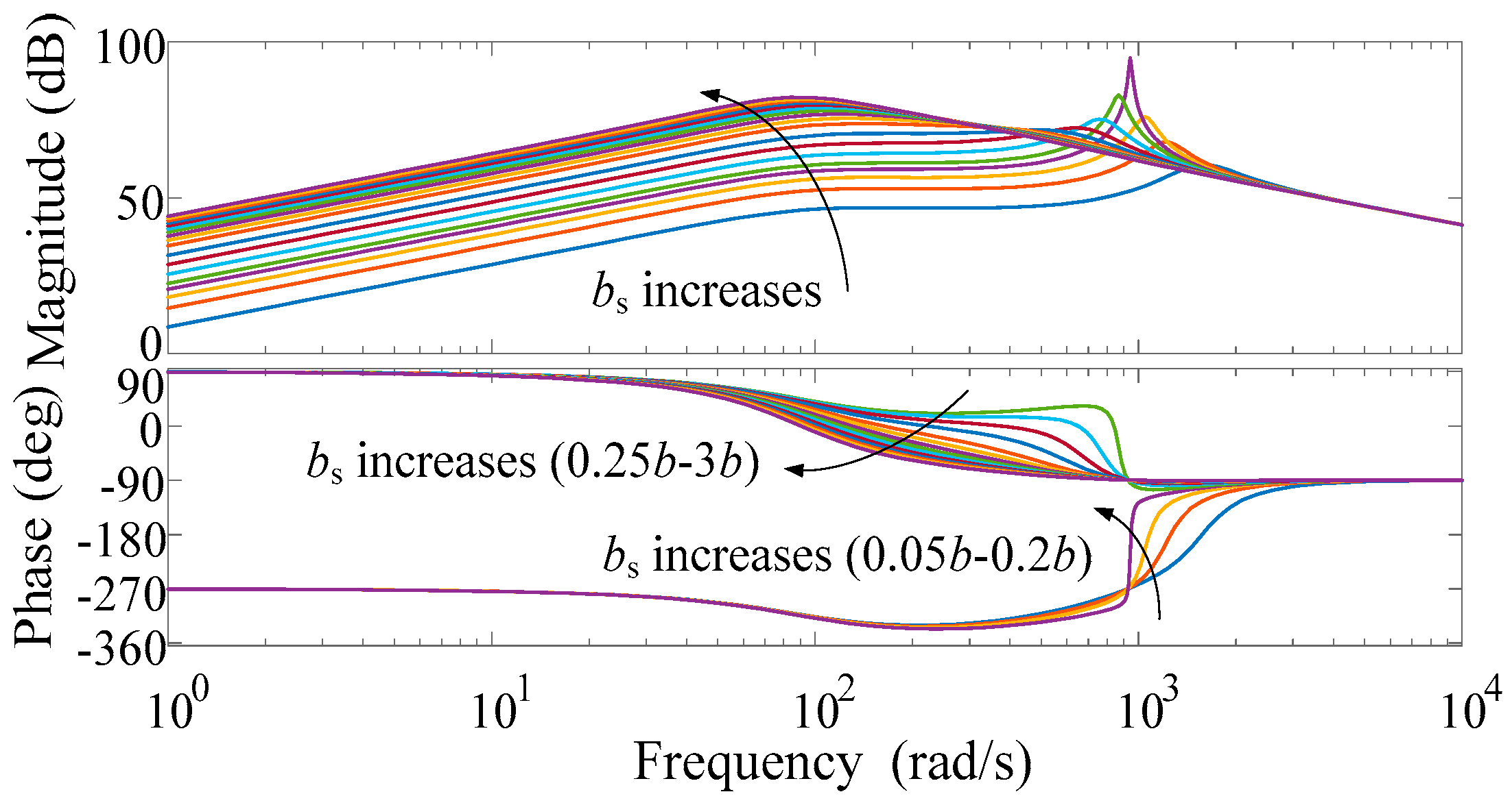
• The appropriate initial values for ${\omega }_{\mathrm{o}}$ and ${\omega }_{\mathrm{c}}$ should not be too large, as stated in the constraints given before. If the dynamic response speed is slow or the capability needs to be enhanced, ${\omega }_{\mathrm{o}}$ and ${\omega }_{\mathrm{c}}$ can be increased until the overshoot exists or the influence of high-frequency noise is obvious.
• Owing to ${\omega }_{\mathrm{o}}$ having a more pronounced influence on the dynamic performance of the system, we can reduce ${\omega }_{\mathrm{o}}$ first until the overshoot disappears or the influence of noise is controllable. Then, we can increase ${\omega }_{\mathrm{c}}$ until the overshoot exists or the influence of the noise is obvious. After this, the tuning sequences can be exchanged until the ideal performance requirement is met.
• If the gain of the controlled object is not clear, the reasonable initial value for $b_{\mathrm{s}}$ should not be too small for stability consideration. If the system is unstable, we can increase $b_{\mathrm{s}}$. Besides, if the capability of rejecting the disturbance needs to be enhanced, we can then decrease $b_{\mathrm{s}}$.

4.2. Robust Performance Concerning

As far as the robustness of the control system is concerned, we can deduce the sensitivity function $S(s)$ and the complementary sensitivity function $T(s)$ of the system as [32,33]:

$$S(s)=\frac{Q\left(s\right)-N\left(s\right)}{Q\left(s\right)}$$

(38)

$$T(s)=\frac{N\left(s\right)}{Q\left(s\right)}$$

(39)

The necessary and sufficient condition for the uncertain system’s robust stability is:

$$\forall \omega >0,T(j\omega )<\frac{1}{\left|\Delta (j\omega )\right|}$$

(40)

For application, the maximum magnitudes of $S(s)$ and $T(s)$ are denoted as:

$$M_{\mathrm{S}}=\underset{\omega >0}{\max }\left|S(j\omega )\right|$$

(41)

$$M_{\mathrm{T}}=\underset{\omega >0}{\max }\left|T(j\omega )\right|$$

(42)

As obtained in previous work [34], the range of $M_{\mathrm{S}}$ is from 1.2 to 2.0 and the corresponding range of $M_{\mathrm{T}}$ is from 1 to 1.5. It is known that a smaller $M_{\mathrm{S}}$ can make the output of the system more insensitive to the uncertainties of the controlled plant, which can strengthen the system’s stability. If a model is not precise enough, the reasonable values of $M_{\mathrm{S}}$ and $M_{\mathrm{T}}$ are recommended as smaller values in a previous study [35]. Based on the above discussions, to guarantee robust operation, $M_{\mathrm{S}}$ is determined during the range from 1.1 to 1.2 and $M_{\mathrm{T}}$ is determined during the range from 1 to 1.5. On the basis of above analysis, we let ${\omega }_{\mathrm{o}}=420$ and ${\omega }_{\mathrm{c}}=70$, so that $M_{\mathrm{S}}=1.14$ and $M_{\mathrm{T}}=1$. The robustness can be guaranteed and the robust performance of the system will be further testified in Section 5 under the condition that the parameter of the controlled object perturbates.

5. Case Study

For clarification of this control approach, here we can include the operating procedures of the improved VSG based on the proposed control strategy in this article (called “LADRC-VSG”). Figure 14 shows the flow chart of the operation of LADRC-VSG.

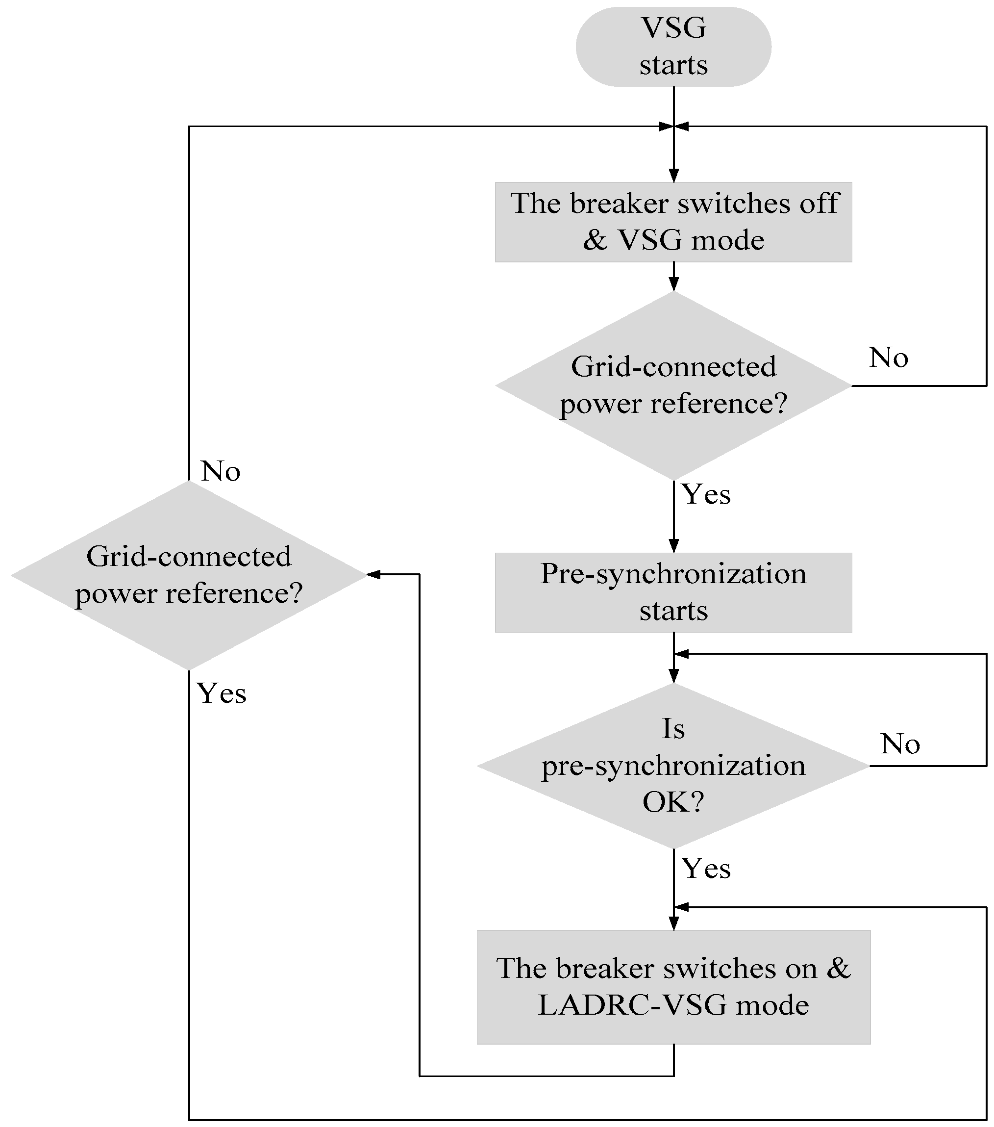
• The VSG starts.
• The VSG runs under island-mode and the breaker maintains “off” status. Meanwhile, the controller detects the grid-connected power reference. If the grid-connected power reference does not exist, continue with Step 2, otherwise the pre-synchronization starts and we proceed to the next step.
• The system judges whether pre-synchronization is completed or not. If it is uncompleted, the procedure continues pre-synchronization, or else it moves to Step 4.
• The breaker is closed and the inverter runs under the mode of LADRC-VSG. Meanwhile, the system detects whether the grid-connected power reference is still there or not. If it is, the procedure of Step 4 continues, or else it goes back to Step 2.

Simulations are carried out in the MATLAB/Simulink environment to verify the proposed control strategy. The grid is set as an infinite bus power system and the internal impedance of the grid is zero. The dynamic responses are studied separately based on the conventional VSG, the VSG based on setting the grid frequency measured by PLL as the frequency reference of VSG [36] (called “PLL-VSG”), and LADRC-VSG. The initial phase angle of the grid voltage is set as ${15}^{\circ }$. Here, $P_{\mathrm{ref}}$ is 0 kW, as is the case in island mode, and $Q_{\mathrm{ref}}$ is 0 kvar. The VSG loads 20 kW at first, $P_{\mathrm{ref}}$ changes to 40 kW at 0.5 s, and it has a step change to 60 kW at 2 s. The lower limit of the control value of LADRC-VSG is set as 25 kW and the total simulation time is 3.5 s.

The simulation cases are divided into two parts, which include the nominal plant in Section 5.1 and the parametric perturbating plant in Section 5.2. Thus, the ability to suppress the disturbance and the robustness of the system will be verified separately. As observed, the cases studied in previous work [15,16] are based on the assumption that the form of grid frequency fluctuation is a step change. Further, the universality of the analysis needs to be considered, thus the cases based on the step change, ramp change, and sinewave form change of grid frequency are studied in Section 5.1, respectively. Moreover, the performance of the mismatching model is studied. The condition of a step change of grid frequency is introduced in detail, and other conditions are illustrated briefly.

5.1. Performance Based on the Nominal Model

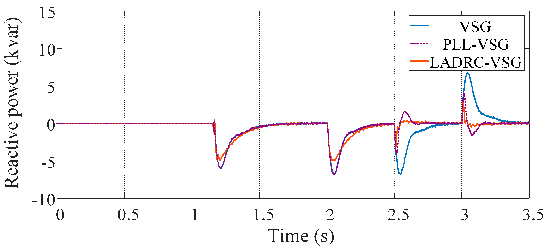
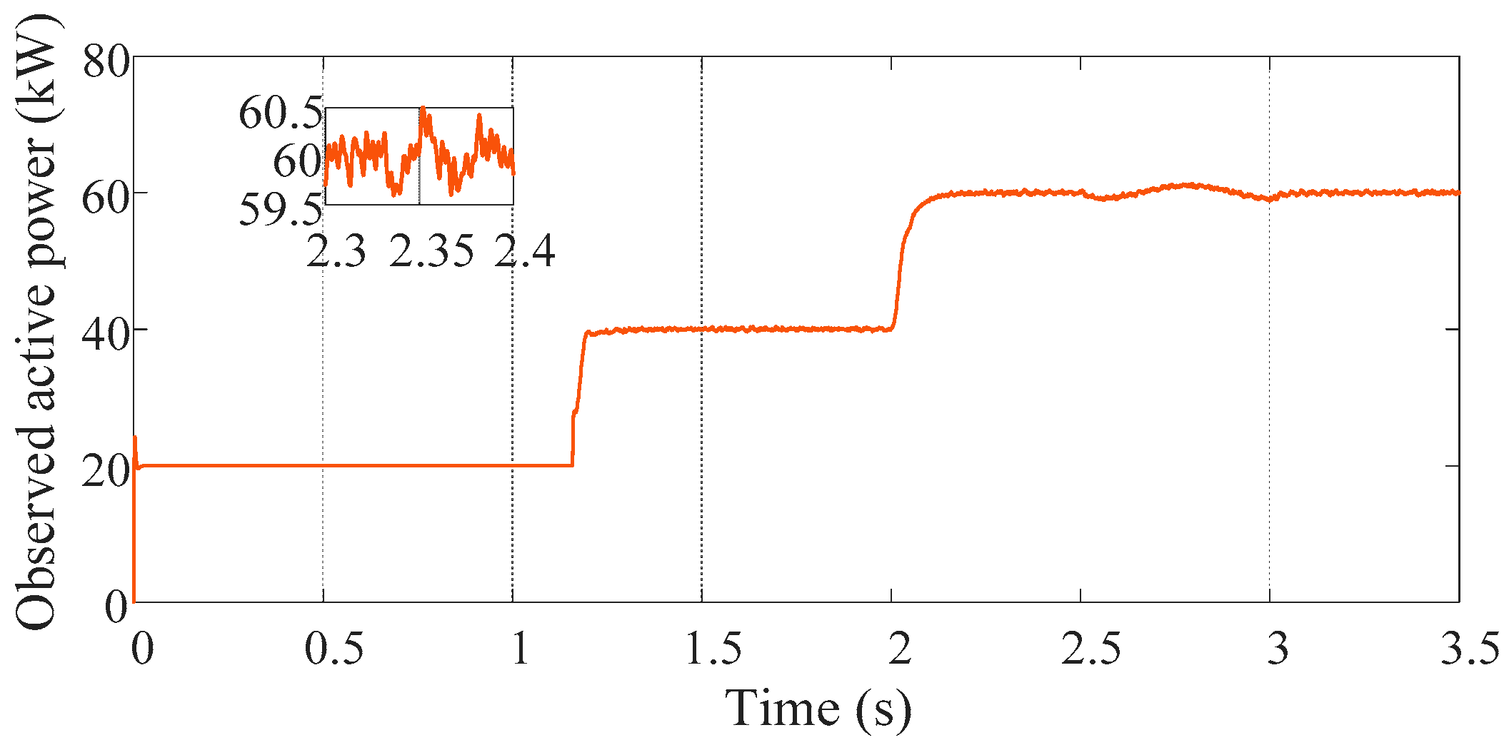
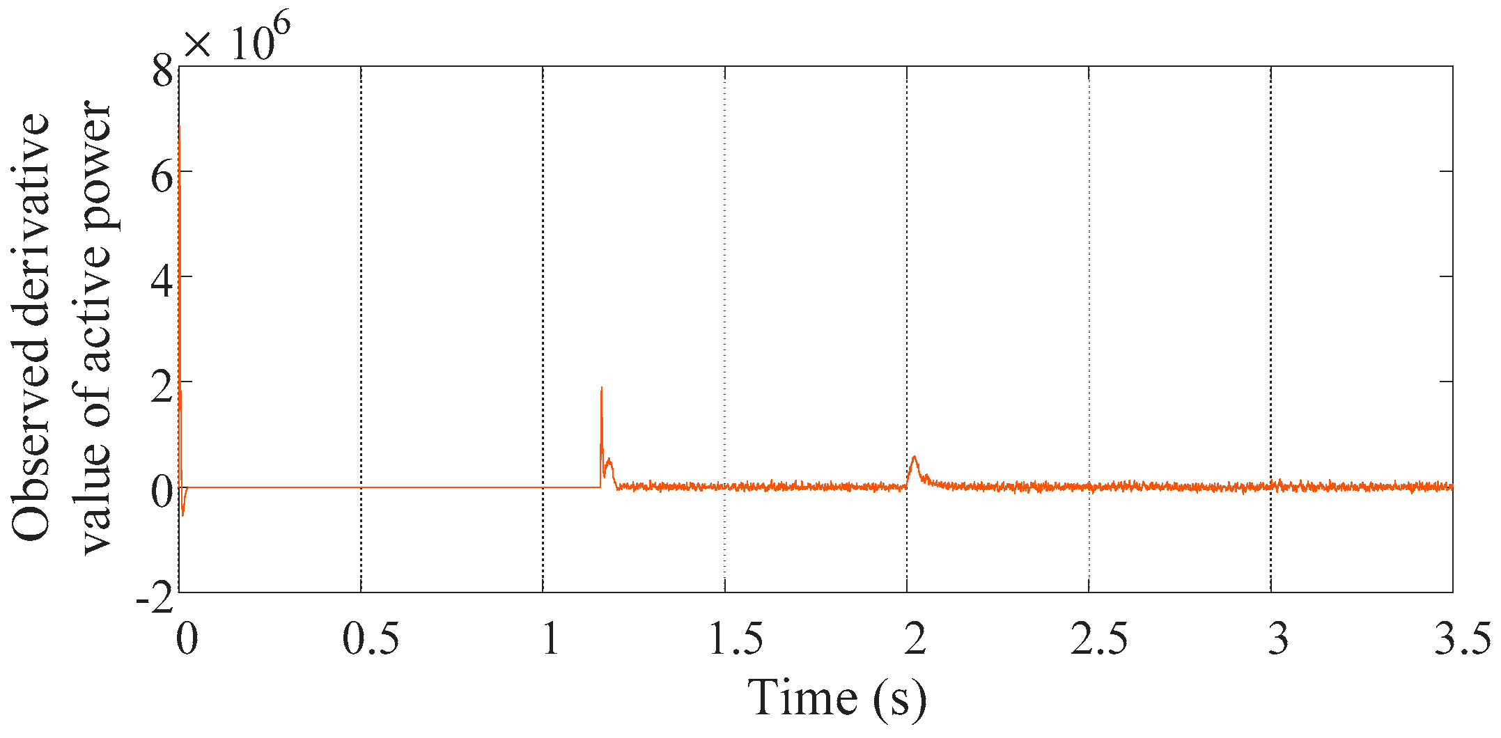
5.1.1. Step Change of Grid Frequency

The grid frequency falls to 49.9 Hz at 2.5 s and is restored to normal at 3 s. The frequency of LADRC-VSG and the grid frequency measured by the PLL are depicted in Figure 15, where the PLL only works during the period of pre-synchronization to acquire the phase angle of the grid voltage before the VSG is connected to the grid. The method for pre-synchronization refers to a previous study [25], in which a PI controller is applied and the maximum frequency reaches the value of 50.7 Hz during the period. Additionally, the PLL withdraws after the switch of the breaker is closed for conventional the VSG and LADRC-VSG. From 0 s to 0.5 s, the inverter runs under the droop mode of VSG and the frequency of VSG is lower than the rated frequency. Pre-synchronization control starts at 0.5 s and the frequency of the VSG is identical to the grid frequency at about 1.16 s, thus VSG is connected to the grid and outputs power according to the power reference from then onwards.

The difference between the conventional VSG and PLL-VSG is that the PLL-VSG adopts the grid frequency as the frequency reference. Therefore, when the frequency does not fluctuate, the conventional VSG shares almost the same waveform with PLL-VSG (0–2.5 s). Figure 16 shows the output power of VSG under different control strategies. From 0 s to 0.5 s, the output power has the same value of 20 kW as the load power. Between 1.16 s and 2 s, the grid frequency is normal and the grid frequency is equal to the VSG reference frequency. Under the condition that the grid frequency is normal (between1.16 s and 2 s), we define

$${\sigma }_{{\mathrm{P}}_{\mathrm{e}}}=\frac{P_{\mathrm{en}}(\max )-P_{\mathrm{ref}}}{P_{\mathrm{ref}}}\times 100\%$$

(43)

Under the circumstance that the grid frequency fluctuates (between 2.5 s and 3 s), we denote that

$$d_{{\mathrm{P}}_{\mathrm{e}}}=P_{\mathrm{ed}}(\max )-P_{\mathrm{ref}}$$

(44)

where ${\sigma }_{{\mathrm{P}}_{\mathrm{e}}}$ is the percent overshoot of $P_{\mathrm{e}}$ and $P_{\mathrm{en}}(\max )$ is the maximum output value of power when the grid frequency is normal (from 1.16 s to 2 s); $d_{P_{\mathrm{e}}}$ is the maximum deviation of $P_{\mathrm{e}}$, and $P_{\mathrm{ed}}(\max )$ is the maximum output value of power when the grid frequency fluctuates (from 2.5 s to 3 s). In Figure 16, we can see that the power overshoot of the conventional VSG and PLL-VSG still exists when connected to the grid with the damping ratio of 0.926. The $P_{\mathrm{en}}(\max )$ of the conventional VSG and PLL-VSG is 43.9 kW and the ${\sigma }_{{\mathrm{P}}_{\mathrm{e}}}$ is 9.7%, whereas obviously LADRC-VSG can track the power reference rapidly with no overshoot, and the ${\sigma }_{{\mathrm{P}}_{\mathrm{e}}}$ of LADRC-VSG is equal to zero. The adjustment time of conventional VSG and PLL-VSG is 0.19 s, which certifies the excellent performance of tracking the power reference of the designed controller. The grid frequency drops by 0.1 Hz from 2.5 s to 3 s, according to Equation (10), and the steady-state power output of the conventional VSG should be 79.74 kW at this time theoretically, which is in agreement with the simulation results. By contrast, the maximum output power of LADRC-VSG is 65.74 kW and there is no oscillation in the dynamic regulation process. As for PLL-VSG, the maximum output power is 69.5 kW. Thus, the $d_{P_{\mathrm{e}}}$ values of LADRC-VSG, conventional VSG, and PLL-VSG are 5.74 kW, 25.13 kW, and 9.5 kW from 2.5 s to 3 s, respectively. In the process of grid frequency recovery, the regulating time of LADRC-VSG is less than 0.1 s, which is lower than that of 0.22 s for conventional VSG and PLL-VSG. Further, it can be seen in Figure 17, under the condition that the active power is controlled precisely, that the oscillation intensity of the reactive power of LADRC-VSG is lower than conventional VSG and PLL-VSG. All of the above results show that LADRC is reliable in power control of the grid-connected VSG.

Figure 18, Figure 19, and Figure 20 show the output current waveforms of LADRC-VSG, conventional VSG, and PLL-VSG, respectively. The output current of VSG under LADRC control strategy has no overshoot and the current is relatively smooth. From 2.5 s to 3 s, the steady-state current of LADRC-VSG is 126.4 A and the current is almost not affected by the fluctuation of grid frequency. At the same time, the steady-state error of current of PLL-VSG can also be eliminated, whereas the maximum output current of the conventional VSG is up to 176 A and the steady-state error of the current is nearly 49.6 A. The goals of disturbance suppression and fast tracking for the power reference without overshoot are achieved.

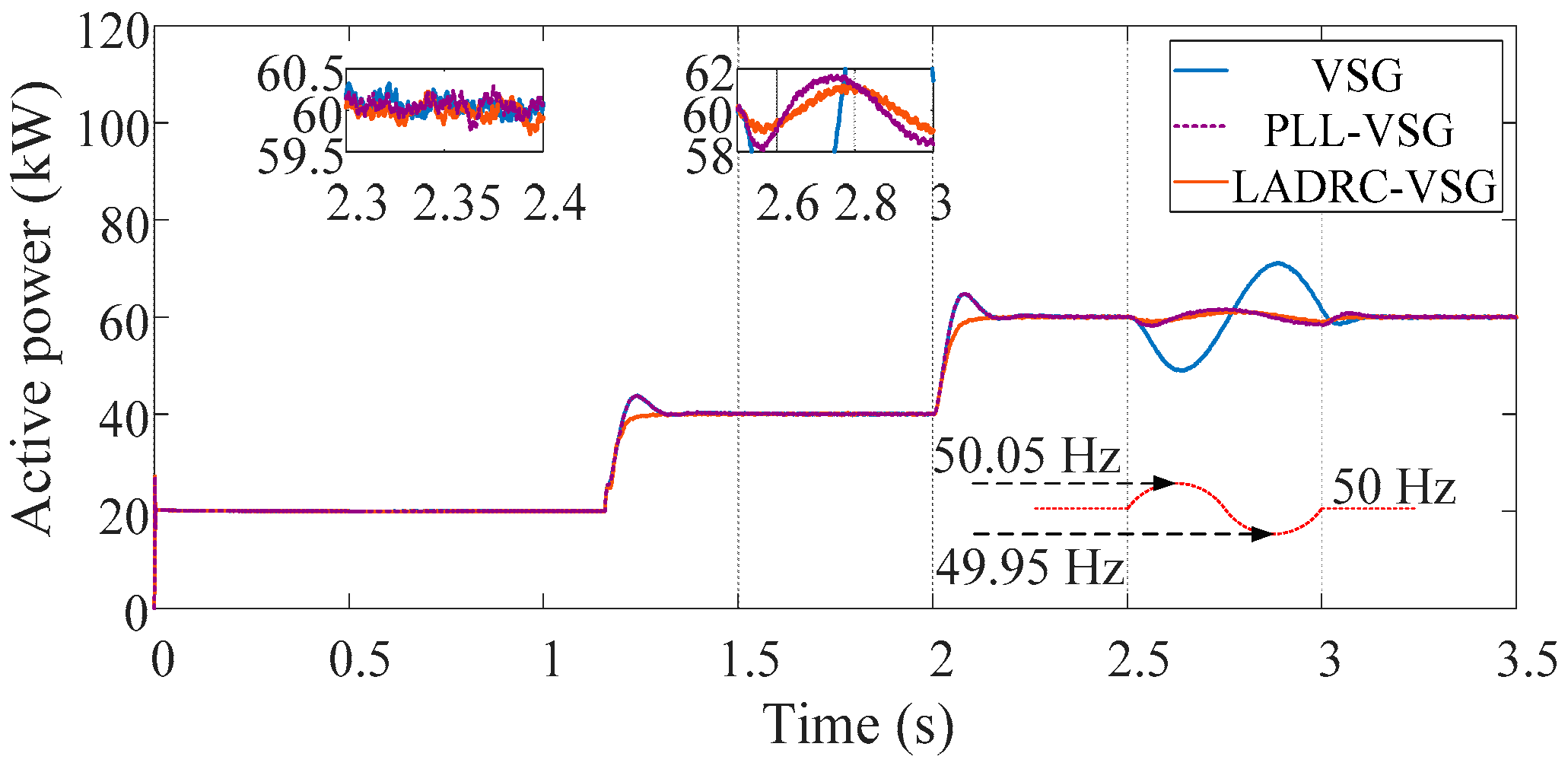
5.1.2. Ramp Change of Grid Frequency

The grid frequency has a ramp change from 50 Hz at 2 s to 49.9 Hz at 2.5 s, and the grid frequency remains at 49.9 Hz after this point. The output active power waveforms of LADRC-VSG, conventional VSG, and PLL-VSG are shown in Figure 21. From 2.5 s to 3 s, the $d_{P_{\mathrm{e}}}$ values of LADRC-VSG, conventional VSG, and PLL-VSG are 0.6 kW, 19.8 kW, and 0.6 kW, respectively. The dynamic error of the power of PLL-VSG and LADRC-VSG is suppressed to a low value and the active power shows no sudden change when the grid frequency fluctuates. At this time, compared with PLL-VSG, the advantage of LADRC-VSG is that it can track the power reference without rapid overshoot.

5.1.3. Sinewave form Change of Grid Frequency

The grid frequency has a sinewave form change with the amplitude of 0.05 Hz at 2 s, which returns to normal at 2.5 s. The cycle of the sinewave form fluctuation is 0.5 s. The performances of LADRC-VSG, conventional VSG, and PLL-VSG can be seen in Figure 22.

The varying angular frequency of disturbance between 2.5 s and 3 s is $2\times 2\times \pi =12.566\mathrm{rad}/\mathrm{s}$ and the output active power of LADRC-VSG has a slight fluctuation. This phenomenon can be explained as the capability to suppress disturbance being reduced because the varying frequency of disturbance increases, and this is consistent with the analysis in Section 4, even though the $d_{P_{\mathrm{e}}}$ of LADRC-VSG is 1.2 kW, which is less than the 10.2 kW value of the conventional VSG and 1.9 kW value of PLL-VSG under the same condition. With different forms of disturbance of frequency, the deviation of power can all be suppressed to an ideal low value, even as low as zero, which reveals that LADRC-VSG is not sensitive to the change of the form of disturbance. The simulations in Section 5.1.1, Section 5.1.2 and Section 5.1.3 convince us that the designed LADRC-VSG controller can reject the external disturbance reliably and it can achieve steady VSG active output power according to the command.

5.2. Control Performance Based on the Parametric Perturbating Model

Section 5.1 reveals the effectiveness of the control method under the condition that the gird frequency has different forms of fluctuation. In real situations, however, the parameters of the filters, the transmission lines, and the inverters may be perturbed for various reasons, such as equipment aging, failure, and other factors. Here, we take the perturbation of the parameter of $L_2$ of the line inductance as an example to illustrate the robust stability of the system.

Here, $L_2$ changes from 0.404 mH to 0.1 mH and the damping ratio ${\xi }_1$ decreases from 0.926 to 0.461. For robustness testing, $b_{\mathrm{s}}$ is not changed in the controller, other simulating conditions are as poor as the conditions in Section 5.1.3, and the grid frequency has a sinewave form change. The amplitude of change is 0.05 Hz and the cycle of the fluctuation is 0.5 s. The grid frequency recovers at 3 s and the simulation results are presented in Figure 23, Figure 24, Figure 25, Figure 26, Figure 27 and Figure 28.

As we can see from Figure 23, with the perturbation of $L_2$, the $P_{\mathrm{en}}(\max )$ values of the conventional VSG and PLL-VSG increases to 54.87 kW between 1.16 s and 2 s, whereas the LADRC-VSG can continue transmitting active power to the grid without overshoot. The ${\sigma }_{{\mathrm{P}}_{\mathrm{e}}}$ values of LADRC-VSG, conventional VSG, and PLL-VSG are 0, 37.17%, and 37.17%, respectively. Additionally, the $d_{P_{\mathrm{e}}}$ values of LADRC-VSG, conventional VSG, and PLL-VSG are 1.44 kW, 11.6 kW, and 4.9 kW, respectively. The adjustment time of LADRC-VSG is 0.12 s, which is much shorter than that the 0.8 s value for conventional VSG and PLL-VSG. LADRC-VSG can output power stably in the case of grid frequency fluctuations, which illustrates the advantage of LADRC, namely that it does not rely on a precise model of the controlled plant. The output reactive power waveforms of LADRC-VSG, conventional VSG, and PLL-VSG are shown in Figure 24. It can be seen that the oscillation of active power will cause instability of the reactive power of conventional VSG and PLL-VSG owing to the presence of coupling between active power and reactive power. Moreover, even though the three control strategies all adopt the method of PI control for reactive power, the better performance of active power of LADRC-VSG causes much less oscillation of reactive power. In addition, the corresponding output angular frequencies of the inverter under different control strategies are shown in Figure 25, where we can see that the angular frequency of LADRC-VSG has better performance. Compared with the performance of the conventional VSG and PLL-VSG, the model mismatching parts in LADRC-VSG can be seen as disturbance, and that can be observed by LESO and compensated by LSEF without delay; thus, the strong robustness can be guaranteed. The estimates for $P_{\mathrm{e}}$ and $\mathrm{d}{P}_{\mathrm{e}}/\mathrm{d}t$ and the lumped disturbance are shown in Figure 26, Figure 27 and Figure 28, respectively, where we can see that the observation for $P_{\mathrm{e}}$ is of high-precision and the observed disturbance is unitless, as the disturbance is caused by a gathering of many factors in Figure 28. The simulations carried out can illustrate the stability and robustness of the system further, which testify to the validity of the proposed control strategy. The comparative analyses of the controllers’ index are given in

Table 2. Comparison of $d_{P_{\mathrm{e}}}$ (2.5–3 s, one decimal place reserved).

Type of Disturbance	LADRC-VSG (kW)	VSG (kW)	PLL-VSG (kW)
Step change of frequency	5.7	25.1	9.5
Ramp change of frequency	0.6	19.8	0.6
Sinewave form change of frequency	1.2	10.2	1.9
Model mismatch; Sinewave form change of frequency	1.4	11.6	4.9

and

Table 3. Comparison of ${\sigma }_{{\mathrm{P}}_{\mathrm{e}}}$ (1.16–2 s, one decimal place reserved).

Type of Model	LADRC-VSG (%)	VSG (%)	PLL-VSG (%)
Normal model	0	9.7	9.7
Mismatch model	0	37.2	37.2

.

As seen in the analyses above, LADRC-VSG can track the power reference without overshoot by compensating for the lumped disturbance, even though the model is mismatched. At the same time, it is noteworthy that the steady-state accuracy of the active power is reduced a little when the controlled object is mismatched, which can be perceived when comparing Figure 22 and Figure 23. As shown in the amplified picture in Figure 22, the steady-state output power is between 59.8 kW and 60.2 kW, whereas under the same condition (the grid frequency does not fluctuate between 1.16 s and 2.5 s), it can be observed that the steady-state output power is between 59.5 kW and 60.5 kW in the amplified picture in Figure 23. This phenomenon reveals that we require a relatively more exact value for the gain of the controlled object to achieve better performance of the controller when the precise model of the controlled object has many uncertainties, so that the capability to reject disturbance can be further enhanced.

6. Conclusions

A control strategy for power tracking of a grid-connected VSG based on LADRC is proposed in this article. On the basis of deducing the power equation of the conventional grid-connected VSG, this article clarifies that VSG has some shortcomings in the power regulation period, such as the contradiction between the response speed of the power output and output overshoot. Additionally, the overcurrent of VSG may cause its dispatch from the grid. Hence, the active power control strategy based on LADRC is proposed. The lumped disturbance is compensated, including the simplified part of the model, the influence of the difference of power reference and the output active power and its differential value, and the difference of the angular frequency reference and the grid angular frequency and its differential value. Then, by deriving the transfer function of the second-order LADRC, the equivalent structure of the grid-connected VSG based on LADRC strategy is obtained. After that, the influences of different parameters of LADRC on the dynamic characteristics of the system are analyzed through frequency domain analysis methods and the robust stability of the control system is analyzed further as well. The simulation results show that LADRC has great performance in power control of the grid-connected VSG, which can improve the power quality of the grid-connected inverters. When the grid frequency is normal, LADRC-VSG can output power according to the power reference quickly and without overshoot. Moreover, LADRC-VSG can maintain robust stability when the parameters perturbate and the analyses show that the LADRC-VSG has a greater performance index. The future vision will be focused on the application of LADRC in the pre-synchronization period of VSG and load-sharing control for VSGs in the microgrid.

References

- Engler, A.; Soultanis, N. Droop control in LV-grids. In Proceedings of the 2005 International Conference on Future Power Systems, Amsterdam, The Netherlands, 16–18 November 2005; p. 6. [Google Scholar] [CrossRef]
- Chen, M.R.; Wang, H.; Zeng, G.Q.; Dai, Y.X.; Bi, D.Q. Optimal PQ Control of Grid-Connected Inverters in a Microgrid Based on Adaptive Population Extremal Optimization. Energies 2018, 11, 2107. [Google Scholar] [CrossRef]
- Adhikari, S.; Li, F. Coordinated Vf and PQ control of solar photovoltaic generators with MPPT and battery storage in microgrids. IEEE Trans. Smart Grid 2014, 5, 1270–1281. [Google Scholar] [CrossRef]
- Lopes, J.P.; Moreira, C.L.; Madureira, A.G.; Resende, F.O.; Wu, X.A.; Jayawarna, N.A.; Zhang, Y.A. Control strategies for microgrids emergency operation. In Proceedings of the 2005 International Conference on Future Power Systems, Amsterdam, The Netherlands, 16–18 November 2005; pp. 57–78. [Google Scholar] [CrossRef]
- Beck, H.P.; Hesse, R. Virtual synchronous machine. In Proceedings of the 2007 9th International Conference on Electrical Power Quality and Utilisation, Barcelona, Spain, 9–11 October 2007; pp. 1–6. [Google Scholar] [CrossRef]
- Visscher, K.; De Haan, S.W.H. Virtual synchronous machines (VSG’s) for frequency stabilisation in future grids with a significant share of decentralized generation. In Proceedings of the CIRED Seminar 2008: SmartGrids for Distribution, Frankfurt, Germany, 23–24 June 2008; pp. 1–4. [Google Scholar] [CrossRef]
- Alipoor, J.; Miura, Y.; Ise, T. Power system stabilization using virtual synchronous generator with alternating moment of inertia. IEEE J. Emerg. Sel. Top. Power Electron. 2015, 3, 451–458. [Google Scholar] [CrossRef]
- Vaddipalli, R.K.N.; Lopes, L.A.; Rathore, A.K. Virtual Synchronous Generator with Variable Inertia Emulation Via Power Tracking Algorithm. In Proceedings of the 2018 2nd International Conference on Power, Energy and Environment: Towards Smart Technology (ICEPE), Shillong, India, 1–2 June 2018; pp. 1–6. [Google Scholar] [CrossRef]
- Fan, W.; Yan, X.; Hua, T. Adaptive parameter control strategy of VSG for improving system transient stability. In Proceedings of the 2017 IEEE 3rd International Future Energy Electronics Conference and ECCE Asia (IFEEC 2017-ECCE Asia), Kaohsiung, Taiwan, 3–7 June 2017; pp. 2053–2058. [Google Scholar] [CrossRef]
- Li, D.; Zhu, Q.; Lin, S.; Bian, X.Y. A self-adaptive inertia and damping combination control of VSG to support frequency stability. IEEE Trans. Energy Convers. 2017, 32, 397–398. [Google Scholar] [CrossRef]
- Rahman, F.S.; Kerdphol, T.; Watanabe, M.; Mitani, Y. Optimization of virtual inertia considering system frequency protection scheme. Electr. Power Syst. Res. 2019, 170, 294–302. [Google Scholar] [CrossRef]
- Haizhen, X.; Xing, Z.; Fang, L.; Fubin, M.; Rongliang, S.; Hua, N. An improved virtual synchronous generator algorithm for system stability enhancement. In Proceedings of the 2015 IEEE 2nd International Future Energy Electronics Conference (IFEEC), Taipei, Taiwan, 1–4 November 2015; pp. 1–6. [Google Scholar] [CrossRef]
- Xu, H.; Zhang, X.; Liu, F.; Mao, F.; Shi, R.; Yu, C.; Yu, Y. Virtual Synchronous Generator Control Strategy Based on Lead-lag Link Virtual Inertia. Proc. CSEE 2017, 37, 1918–1926. [Google Scholar] [CrossRef]
- Li, X.; Hu, Y.; Shao, Y.; Chen, G. Mechanism analysis and suppression strategies of power oscillation for virtual synchronous generator. In Proceedings of the IECON 2017—43rd Annual Conference of the IEEE Industrial Electronics Society, Beijing, China, 5–8 November 2017; pp. 4955–4960. [Google Scholar] [CrossRef]
- Li, M.; Wang, Y.; Zhou, H.; Hu, W. A phase feedforward based virtual synchronous generator control scheme. In Proceedings of the 2018 IEEE Applied Power Electronics Conference and Exposition (APEC), San Antonio, TX, USA, 4–8 March 2018; pp. 3314–3318. [Google Scholar] [CrossRef]
- Yan, X.; Jia, J.; Li, Z.; Ge, Y. Power Control and Smooth Mode Switchover for Grid-connected Virtual Synchronous Generators. Autom. Electr. Power Syst. 2018, 42, 91–99. [Google Scholar] [CrossRef]
- Shintai, T.; Miura, Y.; Ise, T. Oscillation damping of a distributed generator using a virtual synchronous generator. IEEE Trans. Power Deliv. 2014, 29, 668–676. [Google Scholar] [CrossRef]
- Khan, S.; Bletterie, B.; Anta, A.; Gawlik, W. On Small Signal Frequency Stability under Virtual Inertia and the Role of PLLs. Energies 2018, 11, 2372. [Google Scholar] [CrossRef]
- He, X.; Geng, H.; Yang, G. A generalized design framework of notch filter based frequency-locked loop for three-phase grid voltage. IEEE Trans. Ind. Electron. 2018, 65, 7072–7084. [Google Scholar] [CrossRef]
- Du, H.; Sun, Q.; Cheng, Q.; Ma, D.; Wang, X. An Adaptive Frequency Phase-Locked Loop Based on a Third Order Generalized Integral. Energies 2019, 12, 309. [Google Scholar] [CrossRef]
- Han, J.-Q. Auto-disturbances-rejection controller and its’ applications. Control Decis. 1998, 1, 19–23. [Google Scholar] [CrossRef]
- Han, J. From PID to active disturbance rejection control. IEEE Trans. Ind. Electron. 2009, 56, 900–906. [Google Scholar] [CrossRef]
- Gao, Z. Active disturbance rejection control: A paradigm shift in feedback control system design. In Proceedings of the 2006 American Control Conference, Minneapolis, MN, USA, 14–16 June 2006; p. 7. [Google Scholar] [CrossRef]
- Gao, Z. Scaling and bandwidth-parameterization based controller tuning. In Proceedings of the 2003 American Control Conference, Denver, CO, USA, 4–6 June 2003; pp. 4989–4996. [Google Scholar] [CrossRef]
- Lv, Z.; Sheng, W.; Zhong, Q.; Liu, H.; Zeng, Z.; Yang, L.; Liu, L. Virtual Synchronous Generator and Its Applications in Micro-grid. Proc. CSEE 2014, 34, 2591–2603. [Google Scholar] [CrossRef]
- Shintai, T.; Miura, Y.; Ise, T. Reactive power control for load sharing with virtual synchronous generator control. In Proceedings of the 7th International Power Electronics and Motion Control Conference, Harbin, China, 2–5 June 2012; pp. 846–853. [Google Scholar] [CrossRef]
- Zheng, T.; Chen, L.; Guo, Y.; Mei, S. Comprehensive control strategy of virtual synchronous generator under unbalanced voltage conditions. IET Gener. Transm. Distrib. 2017, 12, 1621–1630. [Google Scholar] [CrossRef]
- Hu, W.; Wu, Z.; Sun, C.; Song, Y.; Yuan, K. Modeling and parameter setting method for grid-connected inverter of energy storage system based on VSG. Electr. Power Autom. Equip. 2018, 13–23. [Google Scholar] [CrossRef]
- Chen, J.; Lundberg, K.H.; Davison, D.E.; Bernstein, D.S. The final value theorem revisited-infinite limits and irrational functions. IEEE Control Syst. Mag. 2007, 27, 97–99. [Google Scholar] [CrossRef]
- Zhang, F.; Chen, X.; Zhang, Y.; Jiang, H. Research on Power Transmission Capability of VSC-HVDC Based on Second Order LADRC. Energy Procedia 2019, 158, 2592–2598. [Google Scholar] [CrossRef]
- Yuan, D.; Ma, X.; Zeng, Q.; Qiu, X. Research on frequency-band characteristics and parameters configuration of linear active disturbance rejection control for second-order systems. Control Theory Appl. 2013, 30, 1630–1640. [Google Scholar] [CrossRef]
- Skogestad, S.; Postlethwaite, I. Multivariable Feedback Control: Analysis and Design, 2nd ed.; Wiley: New York, NY, USA, 2007; p. 22. [Google Scholar]
- Wu, M.; He, Y.; Yu, J. Robust Control Theory; Higher Education Press: Beijing, China, 2010; pp. 24–32. [Google Scholar]
- Åström, K.J.; Panagopoulos, H.; Hägglund, T. Design of PI controllers based on non-convex optimization. Automatica 1998, 34, 585–601. [Google Scholar] [CrossRef]
- Sun, L.; Li, D.; Gao, Z.; Yang, Z.; Zhao, S. Combined feedforward and model-assisted active disturbance rejection control for non-minimum phase system. ISA Trans. 2016, 64, 24–33. [Google Scholar] [CrossRef] [PubMed]
- Liu, F. Research on Microgrid Inverter Control Strategy Based on Virtual Synchronous Generator. Ph.D. Thesis, Hefei University of Technology, Hefei, China, April 2015. [Google Scholar]