Optimal Control of Wind Farms for Coordinated TSO-DSO Reactive Power Management

Abstract
:1. Introduction
1.1. Motivation
1.2. State-of-the-Art
1.3. Contribution of This Paper
2. Mathematical Model of the OPF Tool
2.1. Synchronous Generators Model
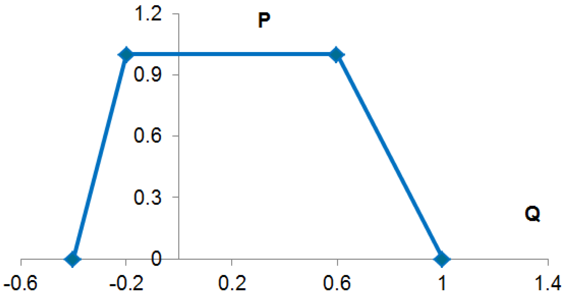
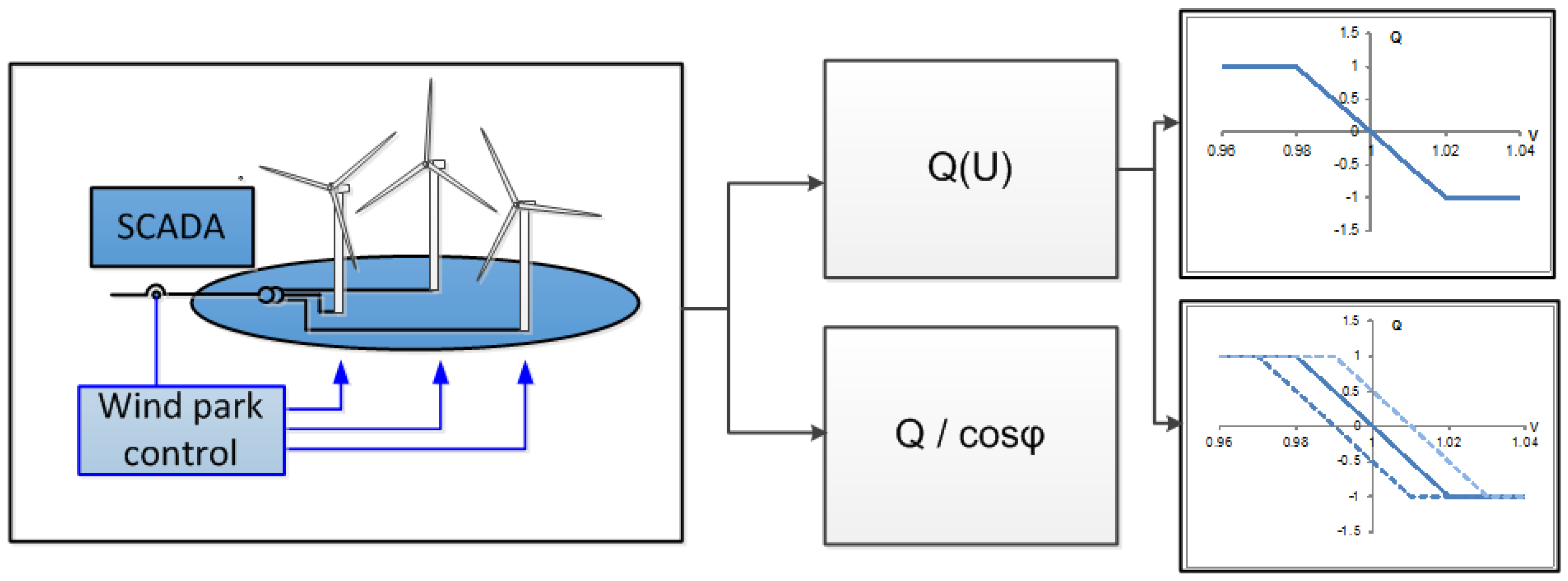
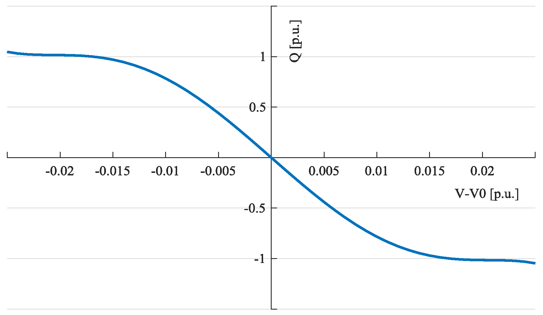
2.2. Wind Farm Control Modes
2.3. Model Predictive Control (MPC)
3. TSO-DSO Coordinated Voltage Control
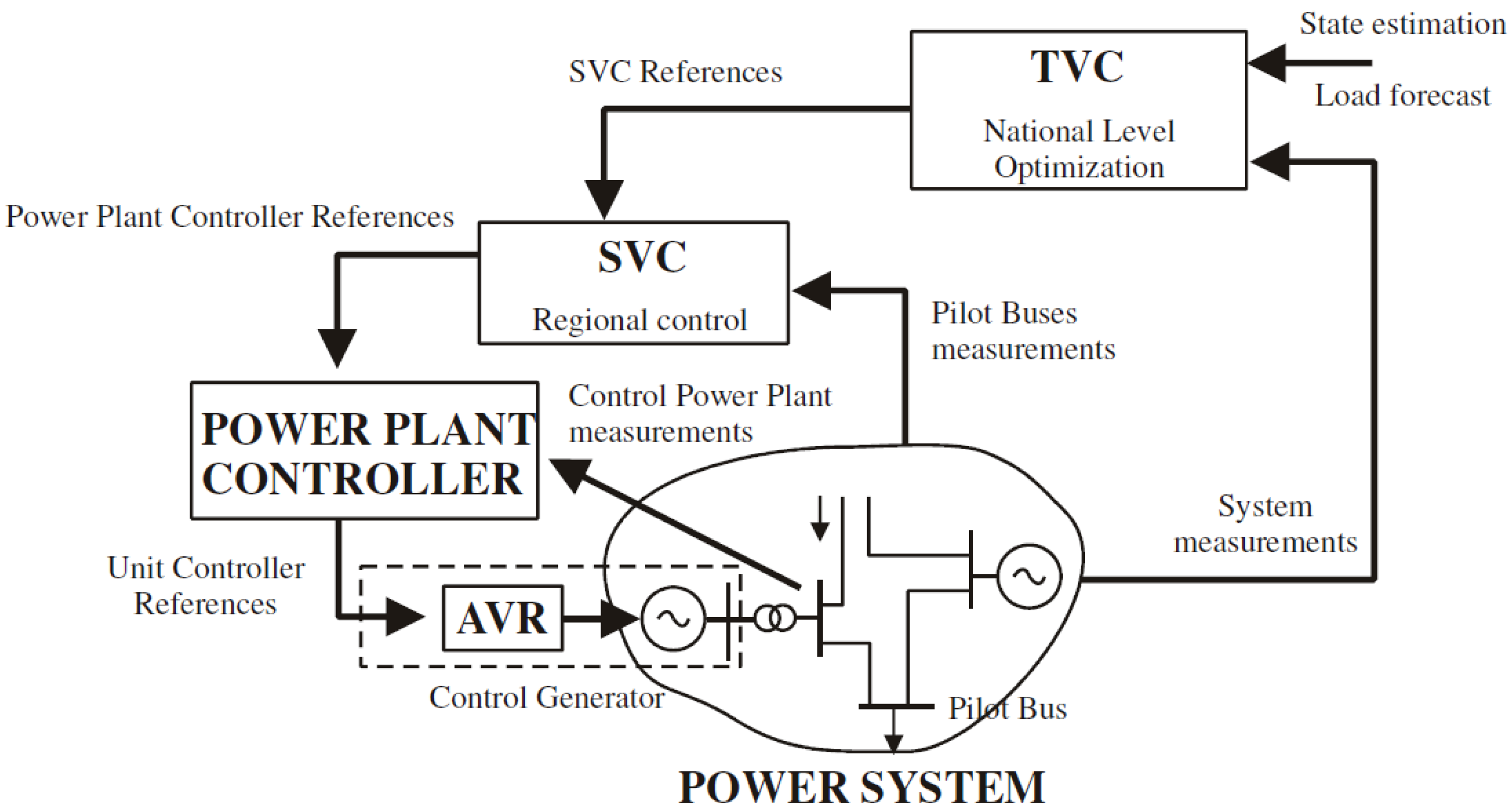
3.1. Overview of Different Voltage Control Methods in the Transmission System
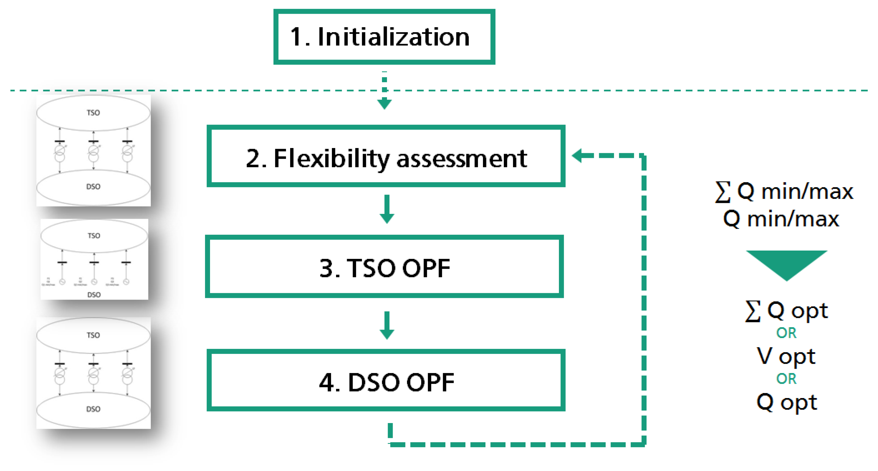
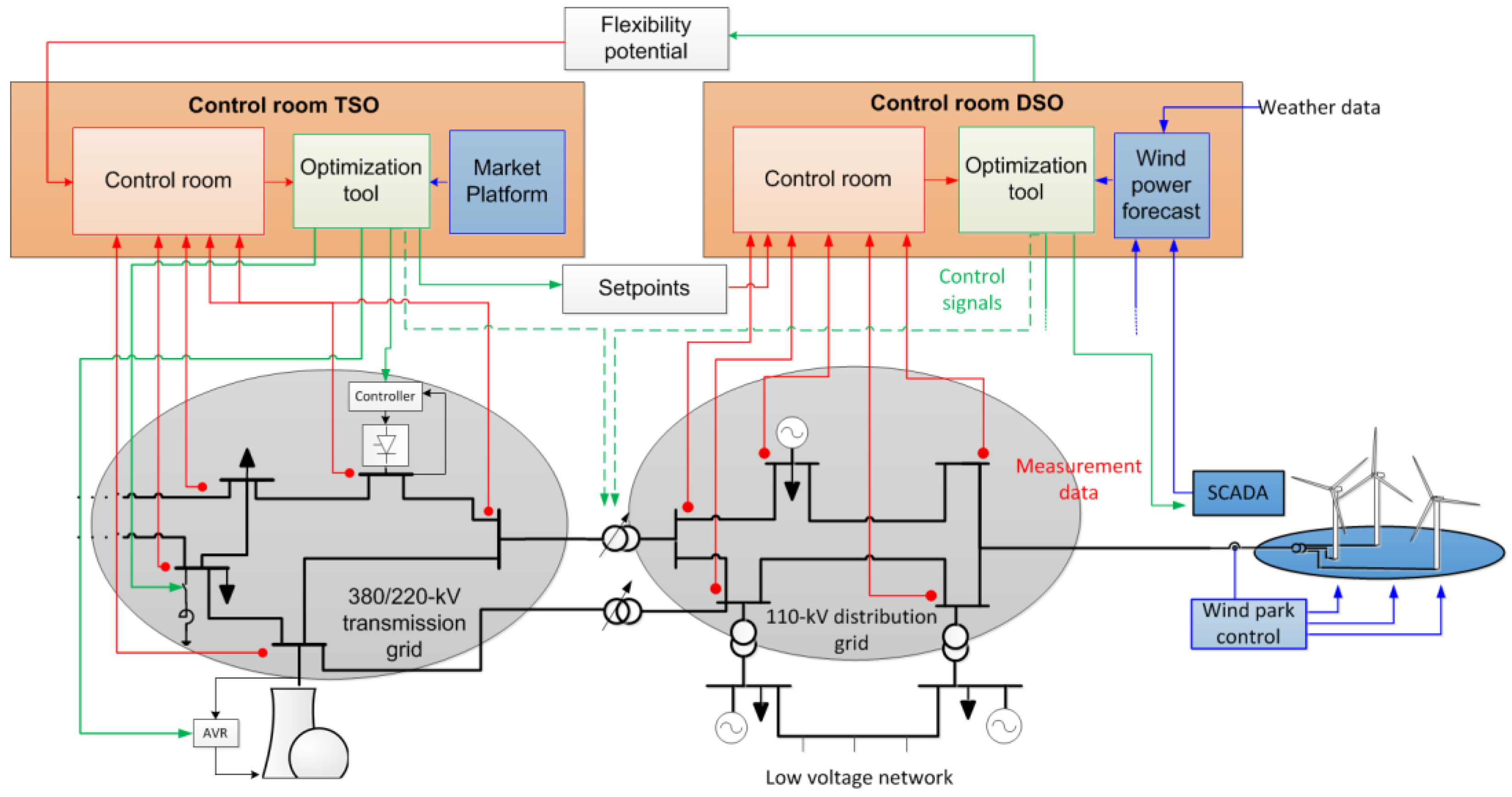
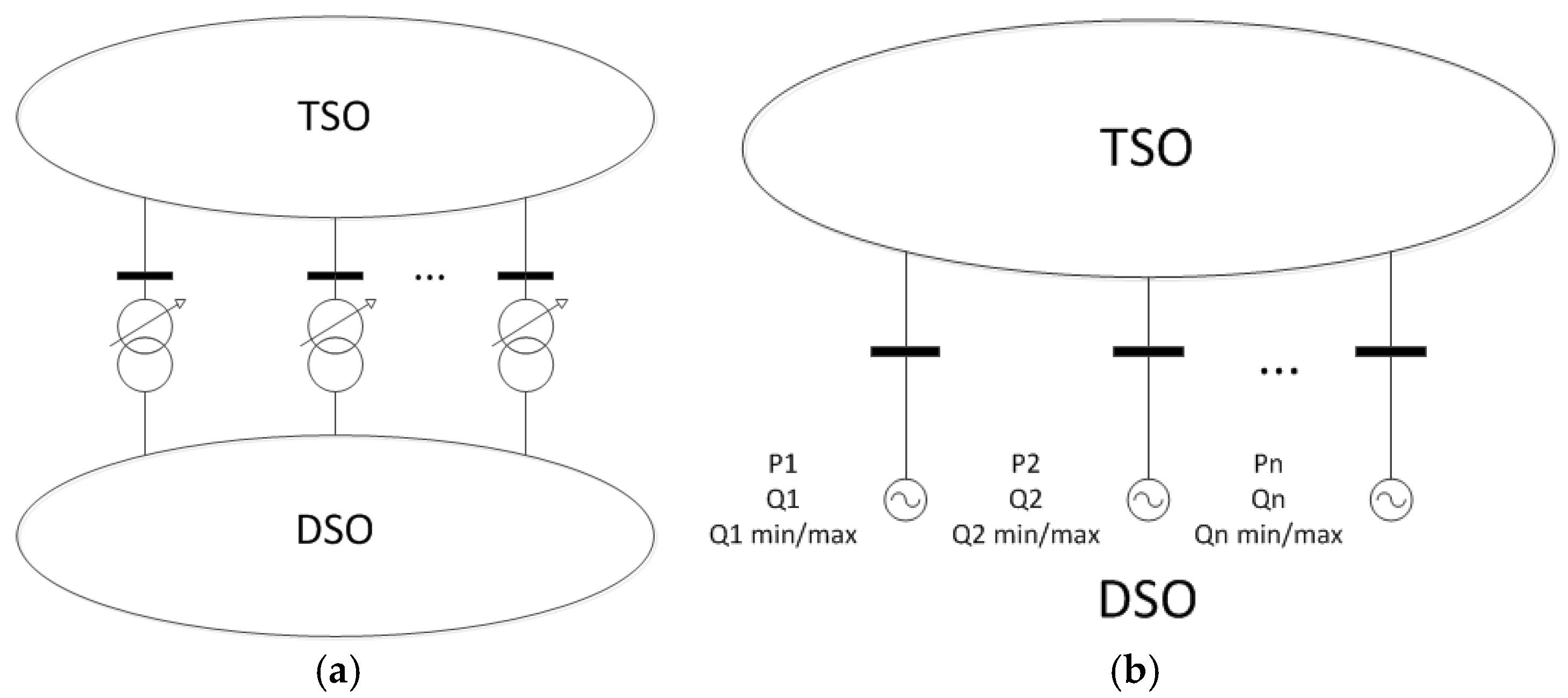
3.2. Coordination Procedure between TSO and DSO
3.2.1. DSO Flexibility Assessment
3.2.2. TSO OPF
3.2.3. DSO OPF
4. Simulation Setup
4.1. Grid Model
4.2. Time Series Data
4.3. Investigated Scenarios
5. Results and Discussion
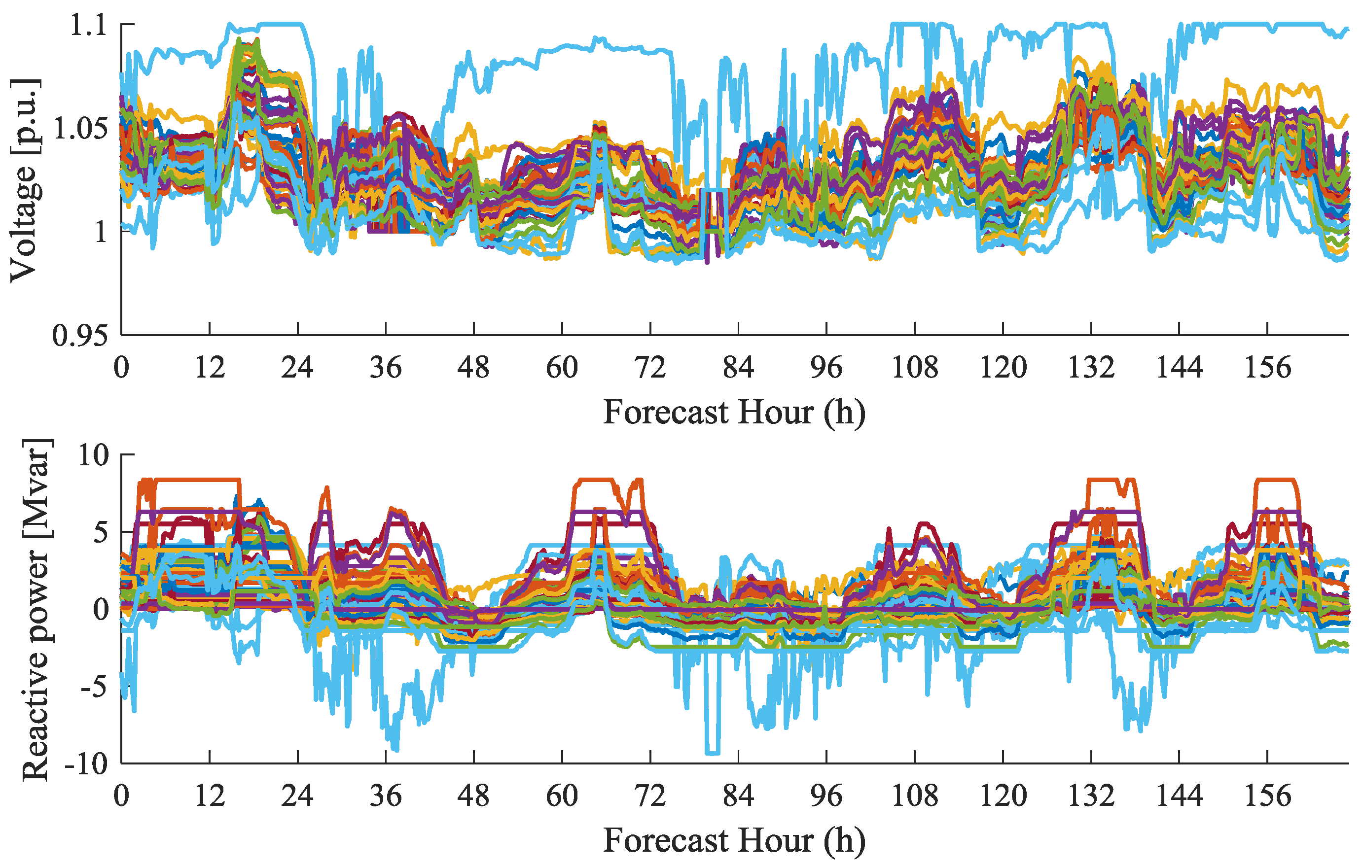
5.1. Feasibility and Performance of Different Setpoints
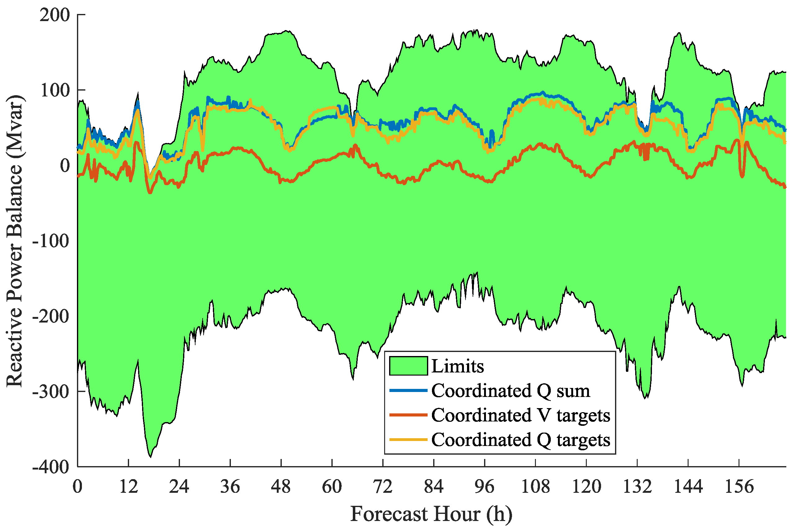
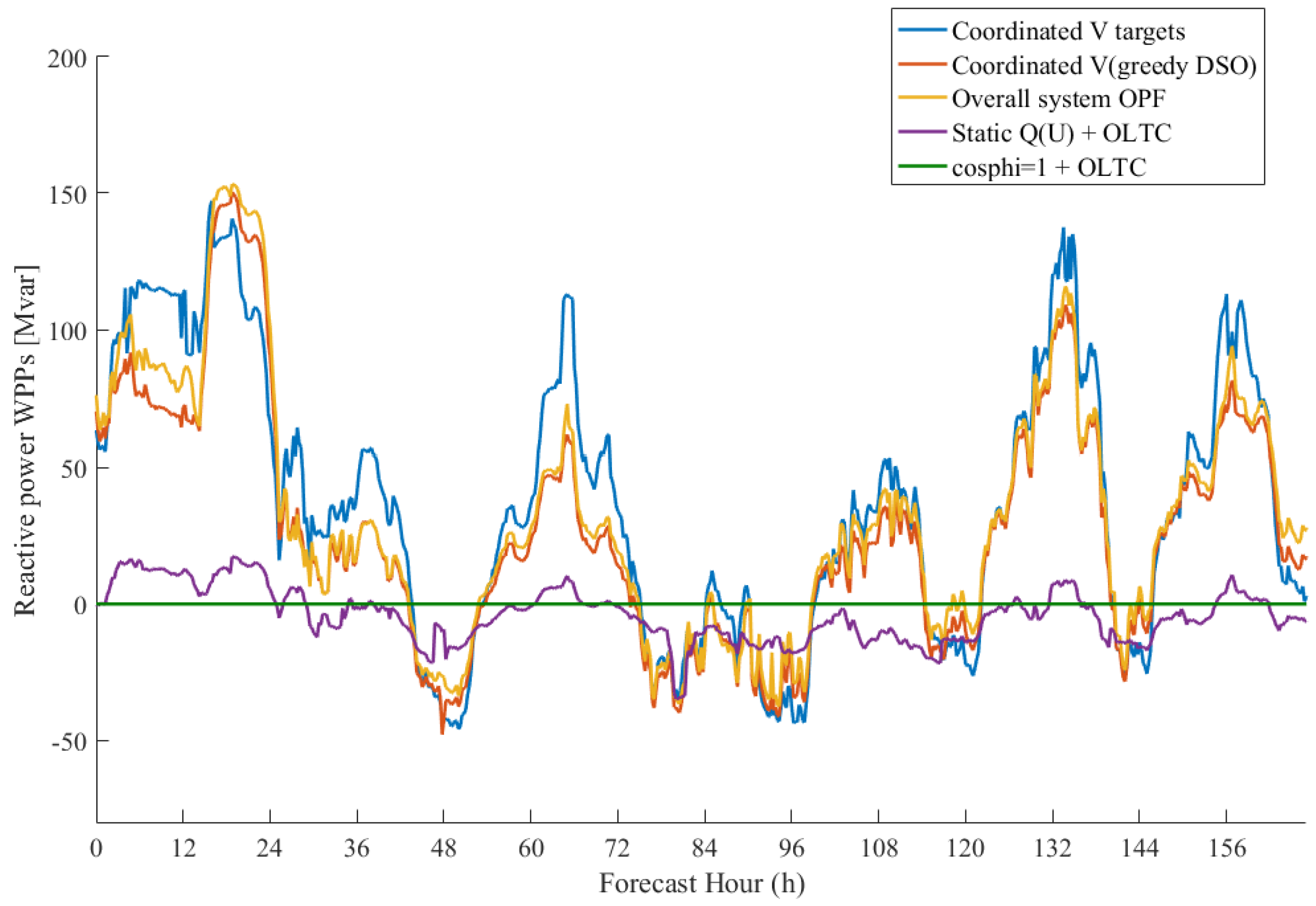
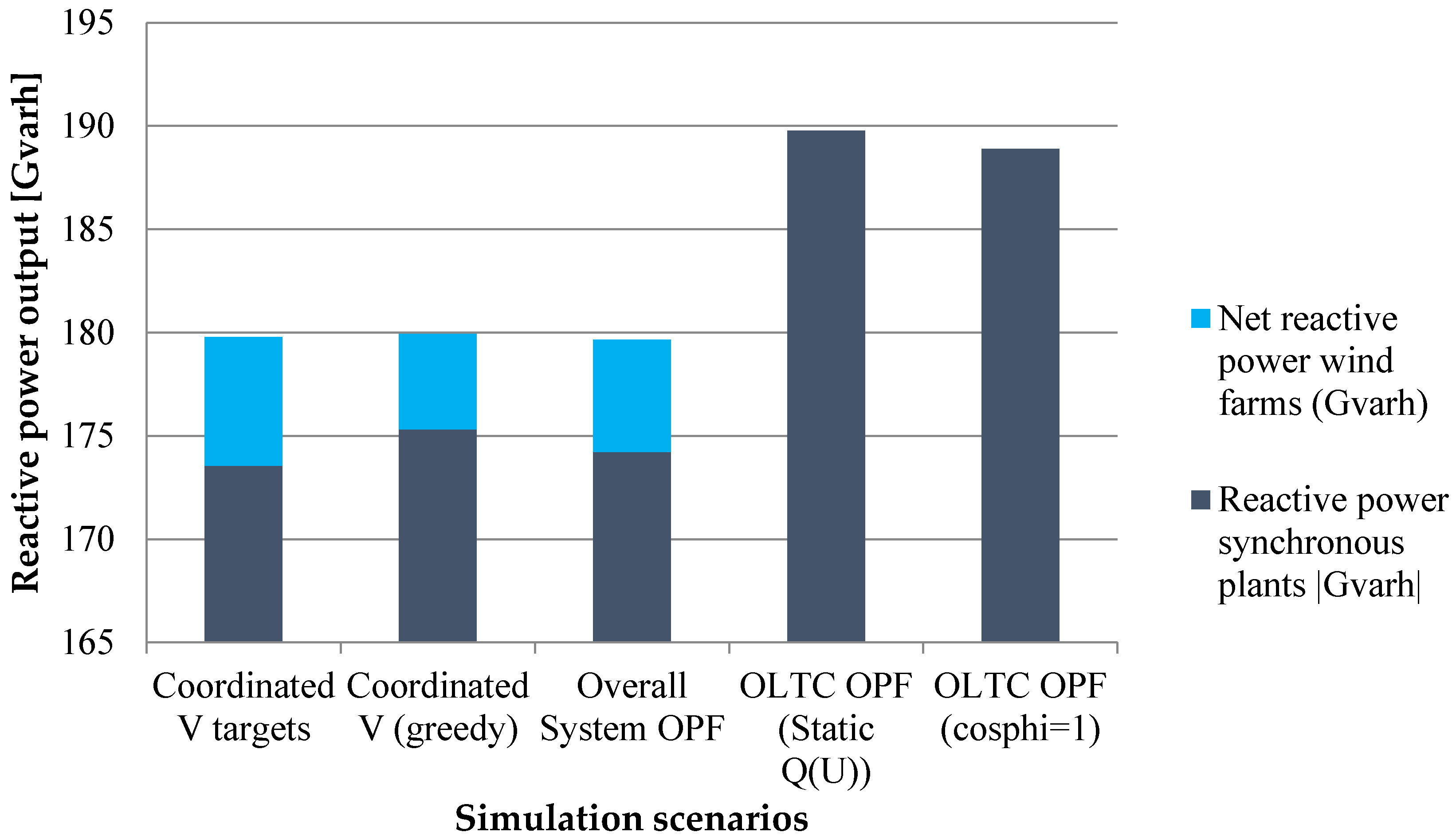
5.2. Performance of Coordinated Optimization with Different DSO Strategies
6. Conclusions
Acknowledgments
Author Contributions
Conflicts of Interest
Nomenclature
| Acronyms | |
| AVR | Automatic voltage regulator |
| CP | Connection point |
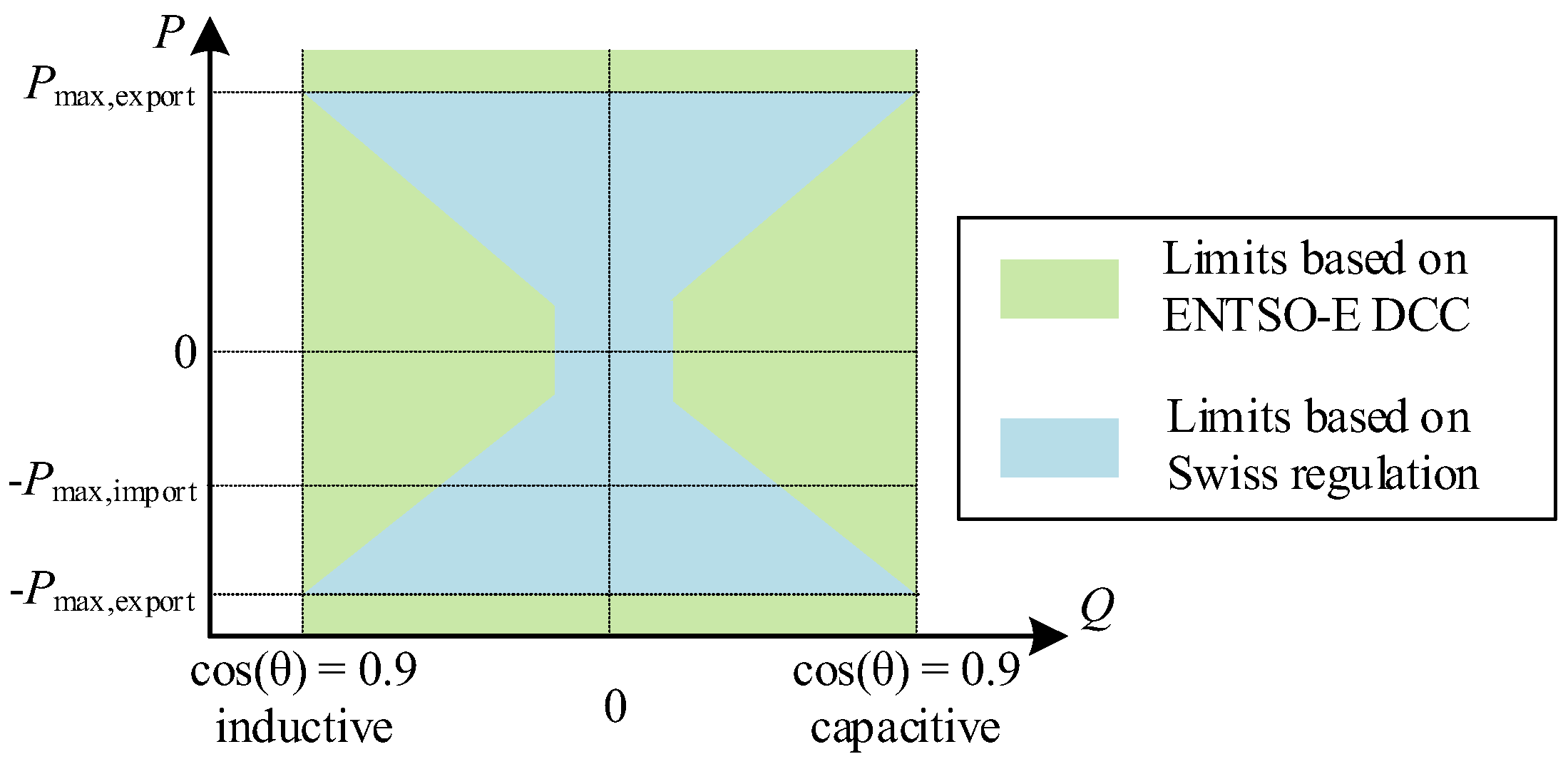
| DCC | Demand and Connection Code |
| DG | Distributed generation |
| DSO | Distribution system operator |
| FACTS | Flexible AC transmission systems |
| HVDC | High Voltage Direct Current |
| ISO | Independent system operator |
| MINLP | Mixed integer-non linear problem |
| MO | Multi-objective |
| MPC | Model predictive control |
| NLP | Non linear problem |
| OF | Objective function |
| OLTC | On load tap changer |
| OPF | Optimal power flow |
| ORPF | Optimal reactive power flow |
| PSO | Particle Swarm Optimization |
| STATCOM | Static Synchronous Compensator |
| UC | Unit commitment |
| TSO | Transmission System Operator |
| VVC | Volt-var control |
| WPP | Wind Power Plant |
| Symbols | |
| A | Areas of optimization |
| B | Susceptance |
| cp | Connection points |
| f | Objective function |
| θ | Angle |
| g | Generator |
| G | Conductance |
| i,j | Nodes |
| K | Boundary nodes (HV side) |
| M | Boundary nodes (EHV side) |
| µ | Objective function weight |
| n | Number of nodes |
| N | Number of connection points |
| opt | Optimal |
| P | Active power |
| Q | Reactive power |
| r | OLTC tap position |
| set | Setpoint |
| t | Time |
| T | MPC time horizon |
| U | Voltage |
| V | Voltage |
Appendix A

| Parameter | Value | Parameter | Value |
|---|---|---|---|
| Maximum load (MW) | 430 | Number of nodes | 167 |
| Maximum total generation (MW) | 1640 | Number of branches | 189 |
| Lower voltage level aggregated generation (MW) | 611 | Number of transmission grid transformers | 8 |
| Controllable wind generation (MW) | 525 | Remaining wind generation (MW) | 505 |
| Parameter | Value | Parameter | Value |
|---|---|---|---|
| Maximum residual load (MW) | 4195 | Number of nodes | 68 |
| Maximum total generation (MW) | 4165 | Number of branches | 104 |
| Number of synchronous generators | 15 | Number of off-shore wind farms | 3 |
| Parameter | Value | Parameter | Value |
|---|---|---|---|
| OLTC capacity range | 100–300 MVA | OLTC estimated cost | 800,000 € |
| Maximum number of operations | 600,000 | Maximum tap operations per 15 min. | 1 |
| Estimated cost of losses | 50 €/MWh | Base [MVA] | 100 |
References
- Ackermann, T.; Andersson, G.; Söder, L. Distributed generation: A definition. Electr. Power Syst. Res. 2001, 57, 195–204. [Google Scholar] [CrossRef]
- Keane, A.; Ochoa, L.F.; Borges, C.L.T.; Ault, G.W.; Alarcon-Rodriguez, A.D.; Currie, R.A.F.; Pilo, F.; Dent, C.; Harrison, G.P. State-of-the-art techniques and challenges ahead for distributed generation planning and optimization. IEEE Trans. Power Syst. 2013, 28, 1493–1502. [Google Scholar] [CrossRef]
- Mousavi, O.A.; Cherkaoui, R. Literature Survey on Fundamental Issues of Voltage and Reactive Power Control; Ecole Polytechnique Fédérale de Lausanne: Lausanne, Switzerland, 2011. [Google Scholar]
- Hinz, F.; Most, D. The effects of reactive power provision from the distribution grid on redispatch cost. In Proceedings of the 2016 13th International Conference on the European Energy Market (EEM), Porto, Portugal, 6–9 June 2016; IEEE: Piscataway, NJ, USA, 2016; pp. 1–6. [Google Scholar]
- Aristidou, P.; Valverde, G.; Van Cutsem, T. Contribution of Distribution Network Control to Voltage Stability: A Case Study. IEEE Trans. Smart Grid 2017, 8, 106–116. [Google Scholar] [CrossRef]
- Morin, J.; Colas, F.; Guillaud, X.; Grenard, S.; Dieulot, J.-Y. Rules based voltage control for distribution networks combined with TSO-DSO reactive power exchanges limitations. In Proceedings of the 2015 IEEE Eindhoven PowerTech, Eindhoven, The Netherlands, 29 June–2 July 2015; IEEE: Piscataway, NJ, USA, 2015; pp. 1–6. [Google Scholar]
- Gabash, A.; Li, P. On Variable Reverse Power Flow-Part I: Active-Reactive Optimal Power Flow with Reactive Power of Wind Stations. Energies 2016, 9, 121. [Google Scholar] [CrossRef]
- Gabash, A.; Li, P. On Variable Reverse Power Flow-Part II: An Electricity Market Model Considering Wind Station Size and Location. Energies 2016, 9, 235. [Google Scholar] [CrossRef]
- Cuffe, P.; Keane, A. Voltage responsive distribution networks: Comparing autonomous and centralized solutions. IEEE Trans. Power Syst. 2015, 30, 2234–2242. [Google Scholar] [CrossRef]
- Kaempf, E.; Abele, H.; Stepanescu, S.; Braun, M. Reactive power provision by distribution system operators—Optimizing use of available flexibility. In Proceedings of the 2014 IEEE PES Innovative Smart Grid Technologies Conference Europe (ISGT-Europe), Istanbul, Turkey, 12–15 October 2014; IEEE: Piscataway, NJ, USA, 2014; pp. 1–5. [Google Scholar]
- Cabadag, R.I.; Schmidt, U.; Schegner, P. The voltage control for reactive power management by decentralized wind farms. In Proceedings of the 2015 IEEE Eindhoven PowerTech, Eindhoven, The Netherlands, 29 June–2 July 2015; IEEE: Piscataway, NJ, USA, 2015; pp. 1–6. [Google Scholar]
- Stock, D.S.; Venzke, A.; Hennig, T.; Hofmann, L. Model predictive control for reactive power management in transmission connected distribution grids. In Proceedings of the 2016 IEEE PES Asia-Pacific Power and Energy Engineering Conference (APPEEC), Xi’an, China, 25–28 October 2016; IEEE: Piscataway, NJ, USA, 2016; pp. 419–423. [Google Scholar]
- EU Commission. Network Code on Demand Connection. Off. J. Eur. Union 2016, 223, 10–55. Available online: Electricity.network-codes.eu/network_codes/dcc/ (accessed on 22 June 2017).
- Valverde, G.; van Cutsem, T. Model Predictive Control of Voltages in Active Distribution Networks. IEEE Trans. Smart Grid 2013, 4, 2152–2161. [Google Scholar] [CrossRef]
- Marten, F.; Lower, L.; Tobermann, J.-C.; Braun, M. Optimizing the reactive power balance between a distribution and transmission grid through iteratively updated grid equivalents. In Proceedings of the 2014 Power Systems Computation Conference, Wroclaw, Poland, 18–22 August 2014; IEEE: Piscataway, NJ, USA, 2014; pp. 1–7. [Google Scholar]
- Zerva, M.; Geidl, M. Contribution of active distribution grids to the coordinated voltage control of the swiss transmission system. In Proceedings of the 2014 Power Systems Computation Conference, Wroclaw, Poland, 18–22 August 2014; IEEE: Piscataway, NJ, USA, 2014; pp. 1–8. [Google Scholar]
- Morin, J. Coordination des Moyens de Réglage de la Tension à L’interface réseau de Distribution et de Transport; et Évolution du Réglage Temps réel de la Tension dans les Réseaux de Distribution. Ph.D. Thesis, dans le cadre de Ecole doctorale Sciences des métiers de l’ingénieur, Paris, France, 2016. [Google Scholar]
- Goergens, P.; Potratz, F.; Godde, M.; Schnettler, A. Determination of the potential to provide reactive power from distribution grids to the transmission grid using optimal power flow. In Proceedings of the 2015 50th International Universities Power Engineering Conference (UPEC), Stoke on Trent, UK, 1–4 September 2015; IEEE: Piscataway, NJ, USA, 2015; pp. 1–6. [Google Scholar]
- Stock, D.S.; Venzke, A.; Lower, L.; Rohrig, K.; Hofmann, L. Optimal reactive power management for transmission connected distribution grid with wind farms. In Proceedings of the 2016 IEEE Innovative Smart Grid Technologies—Asia (ISGT-Asia), Melbourne, Australia, 28 November–1 December 2016; IEEE: Piscataway, NJ, USA, 2016; pp. 1076–1082. [Google Scholar]
- GAMS Development Corporation. General Algebraic Modeling System (GAMS); GAMS Development Corporation: Washington, DC, USA, 2016; Available online: http://www.gams.com/ (accessed on 23 June 2017).
- Byrd, R.H.; Nocedal, J.; Waltz, R.A. Knitro: An Integrated Package for Nonlinear Optimization. In Large-Scale Nonlinear Optimization; Pardalos, P., Di Pillo, G., Roma, M., Eds.; Springer: Boston, MA, USA, 2006; pp. 35–59. [Google Scholar]
- Ilea, V.; Bovo, C.; Merlo, M.; Berizzi, A.; Eremia, M. Reactive power flow optimization in the presence of Secondary Voltage Control. In Proceedings of the 2009 IEEE Bucharest PowerTech, Bucharest, Romania, 28 June–2 July 2009; IEEE: Piscataway, NJ, USA, 2009; pp. 1–8. [Google Scholar]
- Zhu, J. Optimization of Power System Operation, 2nd ed.; IEEE Press/Wiley: Piscataway, NJ, USA, 2015. [Google Scholar]
- Berizzi, A.; Bovo, C.; Allahdadian, J.; Ilea, V.; Merlo, M.; Miotti, A.; Zanellini, F. Innovative automation functions at a substation level to increase res penetration. In Proceedings of the CIGRE 2011 Bologna Symposium—The Electric Power System of the Future: Integrating Supergrids and Microgrids, Bologna, Italy, 13–15 September 2011. [Google Scholar]
- Berizzi, A.; Bovo, C.; Falabretti, D.; Ilea, V.; Merlo, M.; Monfredini, G.; Subasic, M.; Bigoloni, M.; Rochira, I.; Bonera, R. Architecture and functionalities of a smart Distribution Management System. In Proceedings of the 2014 16th International Conference on Harmonics and Quality of Power (ICHQP), Bucharest, Romania, 25–28 May 2014; IEEE: Piscataway, NJ, USA, 2014; pp. 439–443. [Google Scholar]
- Chistyakov, Y.; Kholodova, E.; Netreba, K.; Szabo, A.; Metzger, M. Combined central and local control of reactive power in electrical grids with distributed generation. In Proceedings of the 2012 IEEE International Energy Conference and Exhibition (ENERGYCON), Florence, Italy, 9–12 September 2012; IEEE: Piscataway, NJ, USA, 2012; pp. 325–330. [Google Scholar]
- Corsi, S.; Pozzi, M.; Sabelli, C.; Serrani, A. The Coordinated Automatic Voltage Control of the Italian Transmission Grid—Part I: Reasons of the Choice and Overview of the Consolidated Hierarchical System. IEEE Trans. Power Syst. 2004, 19, 1723–1732. [Google Scholar] [CrossRef]
- Chiandone, M.; Sulligoi, G.; Massucco, S.; Silvestro, F. Hierarchical Voltage Regulation of Transmission Systems with Renewable Power Plants: An overview of the Italian case. In Proceedings of the 3rd Renewable Power Generation Conference (RPG 2014), Naples, Italy, 24–25 September 2014. [Google Scholar]
- Autorità per L’energia Elettrica il Gas e il Sistema Idrico. Regolazione Tariffaria Dell’energia Reattiva per le reti in alta e Altissima Tensione e per le reti di Distribuzione; 420/2016/R/EEL; Autorità per L’energia Elettrica il Gas e il Sistema Idrico: Milan, Italy, 2016; Available online: http://www.autorita.energia.it/it/docs/dc/16/420-16.jsp (accessed on 25 July 2017).
- TenneT TSO GmbH. Grid Code, High and Extra High Voltage; TenneT: Bayereuth, Germany, 2015; Available online: www.tennet.eu/fileadmin/user_upload/The_Electricity_Market/German_Market/Grid_customers/tennet-NAR2015eng.pdf (accessed on 18 September 2017).
- Phulpin, Y.; Begovic, M.; Petit, M.; Heyberger, J.-B.; Ernst, D. Evaluation of network equivalents for voltage optimization in multi-area power systems. IEEE Trans. Power Syst. 2009, 24, 729–743. [Google Scholar] [CrossRef]
- Granada, E.M.; Rider, M.J.; Mantovani, J.R.S.; Shahidehpour, M. Multi-areas optimal reactive power flow. In Proceedings of the 2008 IEEE/PES Transmission and Distribution Conference and Exposition: Latin America, Bogota, Colombia, 13–15 August 2008; IEEE: Piscataway, NJ, USA, 2008; pp. 1–6. [Google Scholar]
- European Commision. EU System Operation Guideline. Establishing a Guideline on Electricity Transmission System Operation; European Commission: Brussels, Belgium, 2016; Available online: ec.europa.eu/energy/sites/ener/files/documents/SystemOperationGuidelinefinal(provisional)04052016.pdf (accessed on 5 July 2017).
- Zhang, W.; Li, F.; Tolbert, L.M. Review of Reactive Power Planning: Objectives, Constraints, and Algorithms. IEEE Trans. Power Syst. 2007, 22, 2177–2186. [Google Scholar] [CrossRef]
- Berizzi, A.; Bovo, C.; Merlo, M.; Delfanti, M. A GA approach to compare ORPF objective functions including Secondary Voltage Regulation. Electr. Power Syst. Res. 2012, 84, 187–194. [Google Scholar] [CrossRef]
- ENTSO-E. REACTIVE POWER MANAGEMENT AT T–D INTERFACE. ENTSO-E Guidance Document for National Implementation for Network Codes on Grid Connection; ENTSO-E: Brussels, Belgium, 2016; Available online: https://www.entsoe.eu/Documents/Network%20codes%20documents/NC%20RfG/161116_IGD_Reactive%20power%20management%20at%20T%20and%20D%20interface_for%20publication.pdf (accessed on 16 June 2017).
- DIgSILENT International. PowerFactory; DIgSILENT International: Gomaringen, Germany, 2016. [Google Scholar]
- The MathWorks Inc. MATLAB; The MathWorks Inc.: Natick, MA, USA, 2016. [Google Scholar]
- VDE|FNN. VDE-AR-N 4120: Technische Anschlussregeln für die Hochspannung. 2017. Available online: www.vde.com/de/fnn/themen/tar/tar-hochspannung/tab-hochspannung-vde-ar-n-4120 (accessed on 18 September 2017).
- Kołodziej, D.; Klucznik, J. Usage of Wind Farms in Voltage and Reactive Power Control Based on the example of Dunowo Substation. Acta Energy 2014, 1, 59–66. [Google Scholar] [CrossRef]
- Mende, D.; Bottger, D.; Ganal, I.; Lower, L.; Harms, Y.; Bofinger, S. Combined power market and power grid modeling: First results of the project SystemKontext. In Proceedings of the 2017 14th International Conference on the European Energy Market (EEM), Dresden, Germany, 6–9 June 2017; IEEE: Piscataway, NJ, USA, 2017; pp. 1–6. [Google Scholar]
- Gerard, H.; Rivero, E.; Six, D. Basic schemes for TSO-DSO Coordination and Ancillary Services Provision. SMARTNET Deliv. D 1.3. 2016. Available online: http://smartnet-project.eu/wp-content/uploads/2016/12/D1.3_20161202_V1.0.pdf (accessed on 28 August 2017).


| Name | DSO Control Variables | Coordination With TSO |
|---|---|---|
| OLTC OPF − cosphi = 1 | OLTC | No |
| OLTC OPF − Static Q(U) | OLTC | No |
| Coordinated Optimization TSO-DSO | OLTC and controllable wind farms | Yes |
| Overall System OPF | Omniscient system operator optimization | |
| Scenario | µlosses | µVP | µΔtap | µΔQ | µΔQcp | µVext |
|---|---|---|---|---|---|---|
| TSO | 1 | 0 | 0 | 0 | 0 | 0 |
| DSO Q sum | 1 | 0 | 0.001 | 1 | 0 | 0 |
| DSO V targets | 1 | 0 | 0.001 | 0 | 0 | 100 |
| DSO Q targets | 1 | 0 | 0.001 | 0 | 0.1 | 0 |
| Scenario | Conneforde 220-kV | Conneforde 380-kV | Emden 220-kV | Emden-Borssum 220-kV | Voslapp 220-kV |
|---|---|---|---|---|---|
| DSO Q sum | 0.088 | 0.114 | 0.704 | 0.682 | 0.022 |
| DSO V targets | 0.176 | 0.304 | 0.088 | 0.088 | 0.220 |
| DSO Q targets | 0.088 | 0.114 | 0.154 | 0.154 | 0.022 |
| Indicator | DSO Q Sum | DSO V Targets | DSO Q Targets |
|---|---|---|---|
| Total reactive power exchange (MVarh) | 9897.46 | 187.52 | 8721.36 |
| Active power losses TSO (MWh) | 5051.60 | 5045.25 | 5052.07 |
| Active power losses DSO (MWh) | 1350.32 | 1335.73 | 1352.66 |
| Total tap changer operations | 33 | 0 | 123 |
| Scenario | µlosses | µVP | µΔtap | µΔQ | µΔQcp | µVext |
|---|---|---|---|---|---|---|
| OLTC OPF-cosphi = 1 | 1 | 0 | 0.001 | 0 | 0 | 0 |
| OLTC OPF-Static Q(U) | 1 | 0 | 0.001 | 0 | 0 | 0 |
| All OPF | 1 | 0 | 0.001 | 0 | 0 | 0 |
| Coordinated V Targets | ||||||
| TSO | 1 | 0 | 0 | 0 | 0 | 0 |
| DSO | 1 | 0 | 0.001 | 0 | 0 | 100 |
| DSO (greedy) | 1.2 | 0 | 0.005 | 0 | 0 | 10 |
| Indicators | Coordinated V Targets | Coordinated V (Greedy) | Overall System OPF | OLTC OPF (Static Q(U)) | OLTC OPF (Cosphi = 1) |
|---|---|---|---|---|---|
| Absolute reactive power exchange (Mvarh) | 187.5 | −1569.5 | −629.9 | −10,163.8 | −9283.8 |
| Reactive power synchronous plants |Gvarh| | 173.56 | 175.33 | 174.23 | 189.77 | 188.90 |
| Net reactive power wind farms (Mvarh) | 6239.12 | 4613.17 | 5432.88 | −707.39 | 0 |
| Active power losses TSO (MWh) | 5045.25 | 5048.17 | 5047.15 | 5082.65 | 5083.31 |
| Active power losses DSO (MWh) | 1335.73 | 1331.56 | 1329.85 | 1374.50 | 1367.25 |
| Average tap changer utilization (%) | 0 | 0.15 | 0 | 0.30 | 1.2 |
| Absolute tap changer operations | 0 | 8 | 0 | 16 | 64 |
| Scenario | Conneforde 220-kV | Conneforde 380-kV | Emden 220-kV | Emden-Borssum 220-kV | Voslapp 220-kV |
|---|---|---|---|---|---|
| DSO V targets | 0.176 | 0.304 | 0.088 | 0.088 | 0.220 |
| DSO V (greedy) | 0.220 | 0.380 | 0.352 | 0.352 | 0.242 |
© 2018 by the authors. Licensee MDPI, Basel, Switzerland. This article is an open access article distributed under the terms and conditions of the Creative Commons Attribution (CC BY) license (http://creativecommons.org/licenses/by/4.0/).
Share and Cite
Stock, D.S.; Sala, F.; Berizzi, A.; Hofmann, L. Optimal Control of Wind Farms for Coordinated TSO-DSO Reactive Power Management. Energies 2018, 11, 173. https://doi.org/10.3390/en11010173
Stock DS, Sala F, Berizzi A, Hofmann L. Optimal Control of Wind Farms for Coordinated TSO-DSO Reactive Power Management. Energies. 2018; 11(1):173. https://doi.org/10.3390/en11010173
Chicago/Turabian StyleStock, David Sebastian, Francesco Sala, Alberto Berizzi, and Lutz Hofmann. 2018. "Optimal Control of Wind Farms for Coordinated TSO-DSO Reactive Power Management" Energies 11, no. 1: 173. https://doi.org/10.3390/en11010173
APA StyleStock, D. S., Sala, F., Berizzi, A., & Hofmann, L. (2018). Optimal Control of Wind Farms for Coordinated TSO-DSO Reactive Power Management. Energies, 11(1), 173. https://doi.org/10.3390/en11010173