The Effect of Fixational Eye Movements on Fixation Identification with a Dispersion-Based Fixation Detection Algorithm

Abstract

Gaze data of 31 participants of a memory recall experiment was analyzed and the I-DT dispersion based algorithm of Salvucci and Goldberg (2000) was used to identify fixations. It was found that individuals differ considerably with regard to the stability of eye gaze and that fixational eye movements affect the accuracy of fixation identification and the optimum dispersion threshold. It was also found that fixation radius and the distance between the points in a fixation that are the furthest apart are the most reliable metrics for a dispersion-based fixation identification algorithm. Finally, it is argued that the correct setting of dispersion threshold is of utmost importance, especially if the participants are not homogeneous with regard to gaze stability.

Introduction

Eye movement is characterized by a series of quick jumps or high velocity movements, known as saccades, followed by fixations, which are periods of time in which the eye is stabilized and remains relatively still. Cognitive processing of a visual stimulus occurs during fixations (Just & Carpenter, 1984) while saccades are considered to be voluntary movements of the eye in order to shift focus from one object of interest to another (Duchowski, 2007).

During fixations, the eye is subject to different types of low velocity movements, namely tremors, drifts and microsaccades (Jacob, 1995; Engbert & Kliegl, 2003; Martinez-Conde et al., 2004). Tremor is a periodic, wave-like motion of the eyes with a typical frequency of ~90 Hz and an amplitude of 20’’ (Martinez-Conde et al., 2004) although occurrences with lower frequency (<40 Hz) and larger amplitude (~10°) have been reported (Leigh, J. R., & Zee, D. S., 1991), especially with reference to certain health conditions (Kennard, 2004). Drifts occur simultaneously with tremor and are slow motions of the eye (0.1-0.5 deg/s) (Martinez-Conde et al., 2004). High-frequency tremor is mostly super-imposed on slow drift (see Martinez-Conde et al. (2004) for an illustrative diagram). Fixational microsaccades are small (~0.3°), fast (~10 deg/s) eye movements that occur involuntarily although they can be voluntarily suppressed (Fiorentini & Ercoles, 1966; Winterson & Collewijn, 1976). They occur intermittently once or twice in a fixation of 300 ms (Martinez-Conde et al., 2004). One of the possible roles of microsaccades is to correct displacements caused by drift, although non-corrective microsaccades occur as well, possibly to prevent visual fading during fixations (Engbert & Kliegl, 2004; Martinez-Conde et al., 2006). A recent review by Collewijn and Kowler (2008) reopens the 50 year old debate about the role of microsaccades by concluding that that microsaccades are neither essential to maintain a stable line of sight, nor for keeping foveal images visible.

The fixation plays a vital role in the analysis of eyetracking data as it allows the analyst to determine where the subject was looking at any given point. Because of the continuous low-velocity eye movements during fixations, fixations are described in terms of the mean x-y coordinate of the gaze position when measured over a minimum period of time during which the gaze does not move further than a predefined maximum distance (Eyenal, 2001). In other words, the so-called point of regard (POR), which is the point in space observed by eye gaze at a specific moment, must remain within a specified area for a specified minimum time in order for it to be regarded as part of a fixation.

Several algorithms exist that can be used to extract fixations from the raw gaze data as reported by an eyetracker (Duchowski, 2007; Jacob, 1990; Jacob, 1993; Salvucci & Goldberg, 2000; Shic et al., 2008; Spakov & Miniotas, 2007). Also, several tools exist that employ these algorithms (Camilli et al., 2008; Eyenal, 2001; Gitelman, 2002; Heminghous & Duchowski, 2006; Salvucci, 2000; Spakov & Miniotas, 2007; Tobii, 2008). In this paper, the focus is on the I-DT dispersionbased algorithm of Salvucci and Goldberg (2000). A software tool has been developed that implements this and several other algorithms.

It has been shown previously that the accuracy of fixation identification algorithms depend heavily on the parameters specified for minimum duration or maximum area (Shic et al., 2008; Blignaut, 2009). Consequently, results produced by different algorithms and parameter settings can have wide-ranging differences (Spakov & Miniotas, 2007). Also, various interpretations and conclusions might be drawn from the same data depending on the parameter settings chosen by the analyst (Shic et al., 2008; Manor & Gordon, 2003).

Besides the accuracy of the scan paths, it was found in a previous paper (Blignaut, 2009) that the number of points of regard included in fixations and the spatial dispersion of PORs within fixations also depend on the threshold setting for a dispersion-based fixation detection algorithm. Furthermore, the optimum threshold for such an algorithm depends on the dispersion metric applied by the algorithm (Blignaut, 2009). In this paper, the scan paths that are returned by a dispersion-based algorithm are compared with a benchmark scan path that is considered to be a good approximation of the actual scan path. Also, the relationship between the amount of fixational eye movements and the optimum threshold and accuracy of scan paths are investigated.

It is hypothesized in this paper that individuals differ from one another with regard to the amount of fixational eye movements and that these differences have an effect on (i) the optimum threshold setting for a dispersionbased fixation detection algorithm and (ii) the accuracy with which fixations can be identified from raw gaze data. If it can be proven that this hypothesis holds in all respects, it is also hypothesized that a common dispersion threshold is not optimal for all participants.

This paper is primarily aimed at practitioners who apply eye-tracking for analysis of gaze behaviour during observation of various kinds of stimuli, e.g. web sites and advertising material. The paper does not intend to contribute to the body of knowledge with regard to the characteristics or physiology of eye movements. The use of a low temporal resolution eye-tracker as was used in this study is, therefore, representative of the typical equipment that is used for, for example, usability analysis of web sites.

Individual differences in fixational eye movements

Observed variability amongst individuals

As a secondary result from an experiment to test the memory recall ability of chess players, it was observed that individuals differ considerably with regard to the stability of their eye gaze (Figure 1). In this experiment 32 participants were presented with an on-screen stimulus showing a typical mid-game setup of a chess game for a period of fifteen seconds. After the fifteen second exposure, participants had to reconstruct the configuration. The recall performance of participants is beyond the scope of this study and only the eye-tracking data that was captured during the fifteen seconds exposure time was analyzed.

As an example, Figure 1 shows recordings of the raw gaze data of two individuals with the chess pieces removed for the sake of clarity. Figure 1a shows the recording of an individual with stable eye gaze while the recording of an individual with a large amount of fixational eye movements is shown in Figure 1b. In Figure 1a the PORs are clustered with a clear distinction between fixations while it is far less obvious to identify fixations from raw gaze data in Figure 1b.

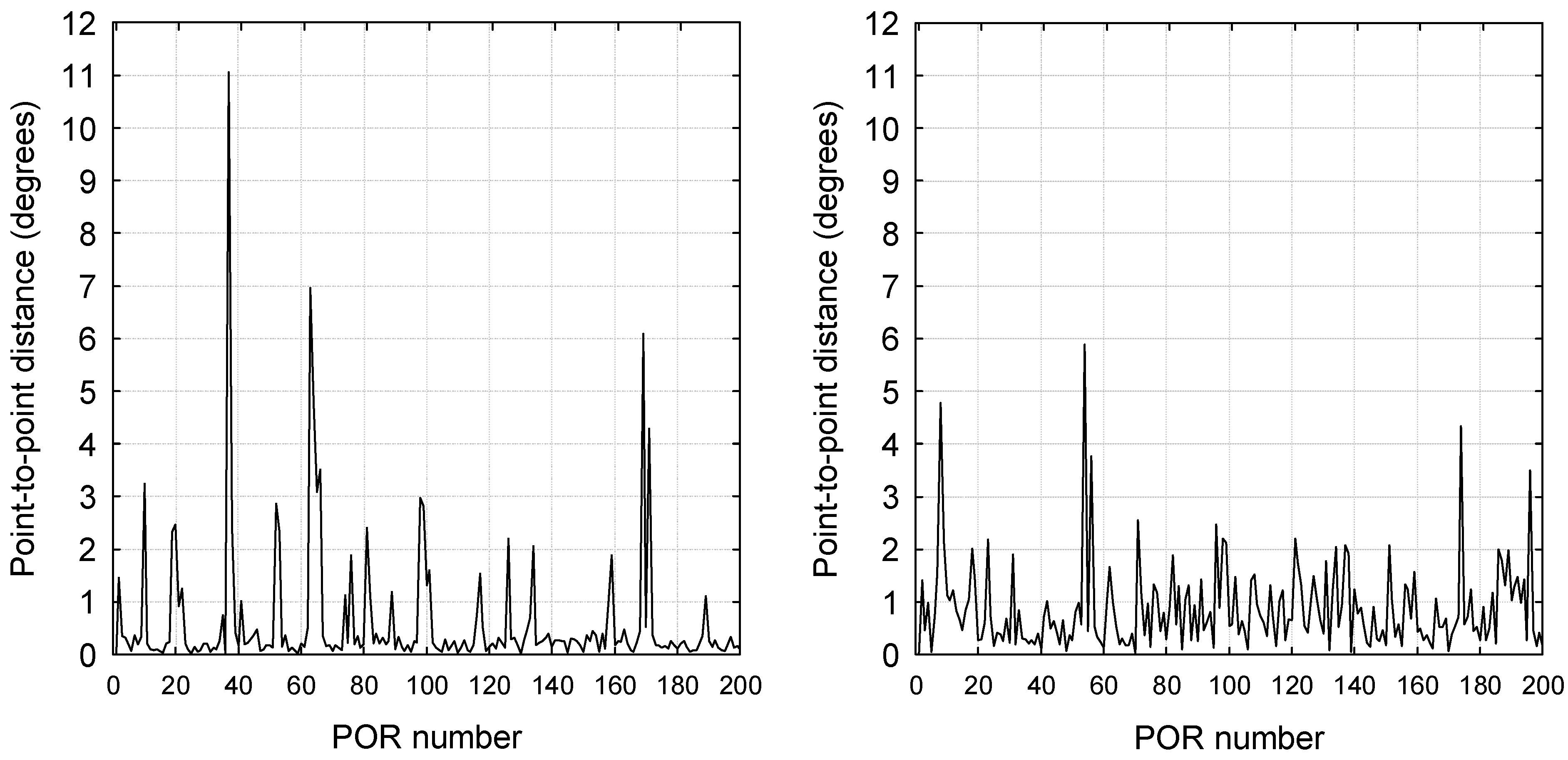
Figure 2 shows the point-to-point distances of the first 200 PORs of the same two recordings as in Figure 1. The peaks indicate saccades while the PORs in between are parts of fixations. The average point-to-point distances within fixations are much higher for the participant with unstable eye gaze than for the one with stable eye gaze. In order to determine if the observations in Figure 1 can be generalized to all participants and expressed quantitatively, the average point-to-point distance of PORs within fixations were determined for each participant. Figure 3 gives a graphical overview of the results.

With regard to the introductory part of the hypothesis stated above, a one-way analysis of variance with participant recording as categorical predictor and the point-to-point distance of PORs within fixations as dependent variable confirmed that people differ significantly from one another with regard to the stability of eye gaze (F(30,18172)=179.33, p<0.001).

Origin of individual differences

The eye is subject to degeneration with age similar to other human organs. Specifically, the macula is a tiny part of the retina and contains the central focusing spot, known as the fovea. It is responsible for seeing details, such as reading, and also for colour vision. Age-related macular degeneration causes a measurable decrease in fixation stability (Timberlake et al., 1986) and an increase in the frequency of ocular tremor (Bolger et al., 2001). Furthermore, the effects of aging cause reductions in light sensitivity, colour perception, dynamic and static visual acuity, and contrast sensitivity (Murata, 2006).

Besides age, several health conditions could be responsible for fixational eye movements with larger-than-normal velocities and duration (Kennard, 2004). Typically, these conditions consist of a drift phase that could last for 200 ms while covering a distance of approximately 10° (velocity ~50 deg/s) followed by a quick correcting saccadic movement that will cover the same distance but in less than 50 ms (velocity >200 deg/s). Some of these conditions, e.g. peripheral vestibular nystagmus and gaze-evoked nystagmus, are fairly common (Dell’Osso & Daroff, 1999), the latter of which requires no treatment as it rarely causes severe visual problems (Kennard, 2004).

Individuals with Alzheimer’s disease are considered to have abnormal fixations with individuals typically fixating on a target and then glancing away and fixating on the target again (Fletcher & Sharpe, 1986). In much the same way, patients with Attention-Deficit Hyperactivity Disorder (ADHD) invariably lack the ability to suppress unwanted saccades and show less ability to control fixations (Munoz et al., 2003).

Discussion of observed variability

Taking into account the spatial resolution of the eyetracker that was used, i.e. 0.25° (Tobii Technology AB, 2003), much of the point-to-point movement within fixations could be ascribed to uncertainty due to equipment limitations and not necessarily to fixational eye movements. For example, the observed point-topoint distances within fixations of the recording of Figure 2a falls well within this limit. For some of the participants, however, the average point-to-point distances were significantly more than could be attributed to equipment limitations and can only be declared in terms of fixational eye movements: tremor, drift and/or microsaccades:

Tremor occurs with a typical frequency of about 90 Hz (Martinez-Conde et al., 2004), meaning that the eyetracker that was used in this study (Tobii 1750, 50Hz) would be unable to pick up individual oscillations.

Although typical drift movements last long enough (minimum 200 ms) to be picked up by this eye-tracker, the maximum reported drift speed of 0.5 deg/s (Martinez-Conde et al., 2004; Engbert & Kliegl, 2004) is well below the minimum average point-to-point velocity of 8.0 deg/s that was observed (Figure 3).

The observed velocity of point-to-point movements ranged from 8 deg/s to 30 deg/s (avg 14.8 deg/s, sd=5.85) which agrees with the typical speed of microsaccades, i.e. ~10 deg/s (Martinez-Conde et al., 2004). Furthermore, the fact that the typical duration (25 ms) and amplitudes (~0.3°) of microsaccades are large enough to be captured by the eye-tracker that was used in this study, suggests that microsaccades could possibly explain the observed point-to-point movements. However, microsaccades normally occur only once or twice in a fixation of 300 ms (Martinez-Conde et al., 2004) while our data shows more frequent point-to-point movements of this order for some individuals.

Therefore, based on the observed data, the characteristics of fixational eye-movements and the limitations of the equipment, the observed point-to-point movements in excess of 0.25° can only be explained in terms of atypical behaviour due to, for example, age or health related conditions as discussed above. In fact, although not enough data was available to do a reliable correlation analysis, it was observed that the three participants with the highest point-to-point velocity (>24 deg/s) were the only three participants over the age of 60.

For the purposes of this paper, it is, however, not important as to why some individuals show atypical behaviour as far as gaze stability is concerned, but rather that there are differences from normal behaviour.

Identification of fixations

Two basic conditions exist for a cluster of PORs to constitute a fixation: The total duration must be long enough and the PORs must be spatially close enough to one another while forming a temporal sequence. These conditions can be more precisely defined in terms of a duration threshold and a distance or velocity threshold.

Existing algorithms for fixation detection

The algorithms that can be used to identify fixations within raw gaze data can roughly be categorized in terms of the way in which the above-mentioned conditions for fixations and the corresponding thresholds are handled. The velocity-threshold algorithm discussed by Salvucci and Goldberg (2000) and Kumar et al. (2008) separates fixation points (PORs belonging to a fixation) and saccadic points (PORs that do not belong to a fixation) based on their point-to-point velocities. The velocity of a fixation point is less than a chosen threshold value while a saccadic point has a velocity that is larger than or equal to the threshold. Thereafter, consecutive fixation points are collapsed into fixations and saccadic points are discarded.

The dispersion-threshold algorithm was originally proposed by Widdel (1984) while adaptations and implementations thereof are discussed in Camilli et al. (2008), Salvucci and Goldberg (2000), Shic et al. (2008) and Urruty et al. (2007). The algorithm utilizes the fact that fixation points, because of their low velocity, tend to cluster close together. Fixations are identified as groups of consecutive PORs within a particular dispersion or maximum separation. Various metrics can be used for dispersion, e.g. the distance between points in the fixation that are the furthest apart (Salvucci & Goldberg, 2000), the distance between any two consecutive points (Shic et al., 2008; Spakov & Miniotas, 2007) and the distance between points and the centre of the fixation (radius) (Camilli et al., 2008; Shic et al., 2008).

Recently, two promising approaches towards fixation detection were proposed: The mean shift procedure proposed by Santella and DeCarlo (2004) searches for a local maximum in a d-dimensional space by shifting each point of the space towards higher density areas in order to separate clusters until such movements involve a small number of points. Urruty et al. (2007) proposed a clustering algorithm in which clusters are formed in subspaces of lower dimensionality which are then used to identify clusters in the original dataset.

Importance of threshold values

One of the biggest restrictions of the available algorithms for fixation detection is the fact that the parameter settings are crucial. Karsh and Breitenbach (1983) have shown that the different algorithms for detecting fixations can lead to totally divergent results. Shic et al. (2008) indicated that the mean fixation duration is a linear function of the parameters chosen. Shic et al. (2008) also showed that specific findings of an eye-tracking analysis can be made insignificant or even reversed by changing parameter settings.

If the duration threshold is set too low, false fixations might be identified; if it is too high, actual fixations might be missed (Camilli et al., 2008). Manor and Gordon (2003) have also shown that significantly more fixations are identified with a duration threshold of 100 ms than with a threshold of 200 ms.

If the dispersion threshold for a dispersion-based algorithm is too low, the algorithm might exclude fixations of people with a large amount of fixational eye movements. If the dispersion threshold is too high, intermediate PORs that are actually part of saccades might be mistaken to be part of a fixation or else separate fixations could be merged.

Duchowski (2007) indicates that parameters may be determined empirically and refers also to Tole and Young (1981) who suggested an adaptive approach to overcome the criticality of threshold values by recalculating the thresholds based on recently observed noise. It might also be possible to personalize the threshold for individual users in order to accommodate individual differences with regard to fixational eye movements (refer to Figure 1a and Figure 1b).

The threshold values for fixation duration and dispersion that are normally used during research are motivated from physiological characteristics. Depending on the nature of the task, it is normally recommended that the threshold for minimum fixation duration is 100-200 ms (Manor & Gordon, 2003) while the dispersion threshold should include a visual angle of 0.5° to 1°, i.e. a radius of 0.25° to 0.5° (Camilli et al., 2008; Eyenal, 2001; Jacob & Karn, 2003; Salvucci & Goldberg, 2000). For stimuli that contain mostly pictures, Tobii Technology (2008) recommends a fixation radius of 50 pixels (1.6° on a 17” eye-tracker with 1024×768 screen resolution at 600 mm viewing distance).

Blignaut (2009) argues that the above-mentioned recommendations are mostly too low and found a radius threshold of between 0.7° and 1.3° to be optimal, i.e. leading to the most accurate identification of scan paths. In this study these results are taken a step further: it was investigated whether individual differences with regard to gaze stability affect the value of the optimum threshold.

Methodology

A software tool was developed to identify fixations from raw gaze data. The tool allows the analyst to choose from several algorithms and set the relevant parameters. The tool also allows the manual identification of fixations from raw data.

For the purposes of this paper the dispersion-threshold algorithm for fixation identification (I-DT) of Salvucci and Goldberg (2000) was used. Six metrics were applied one after the other as a measure of the dispersion of PORs within a fixation. For each metric, a scan path (fixation sequence) was generated for each threshold value in a range of values between 0.2° and 3.0° at regular intervals, e.g. 0.20°, 0.25°, 0.30°, ... , 2.95°, 3.0°.

For each participant, the average point-to-point distance of PORs within a fixation is used as indicator of the amount of fixational eye movements. Accuracy of fixation identification is expressed in terms of the difference between (i) the scan path as identified by the dispersion based algorithm with a specific metric / threshold combination and (ii) the benchmark scan path as identified manually from the raw gaze data.

Details about the participants, stimulus, equipment, the algorithm and metrics used, the procedure to determine the benchmark scan paths as well as the procedure to measure the difference between two scan paths, are discussed below.

Participants and stimulus

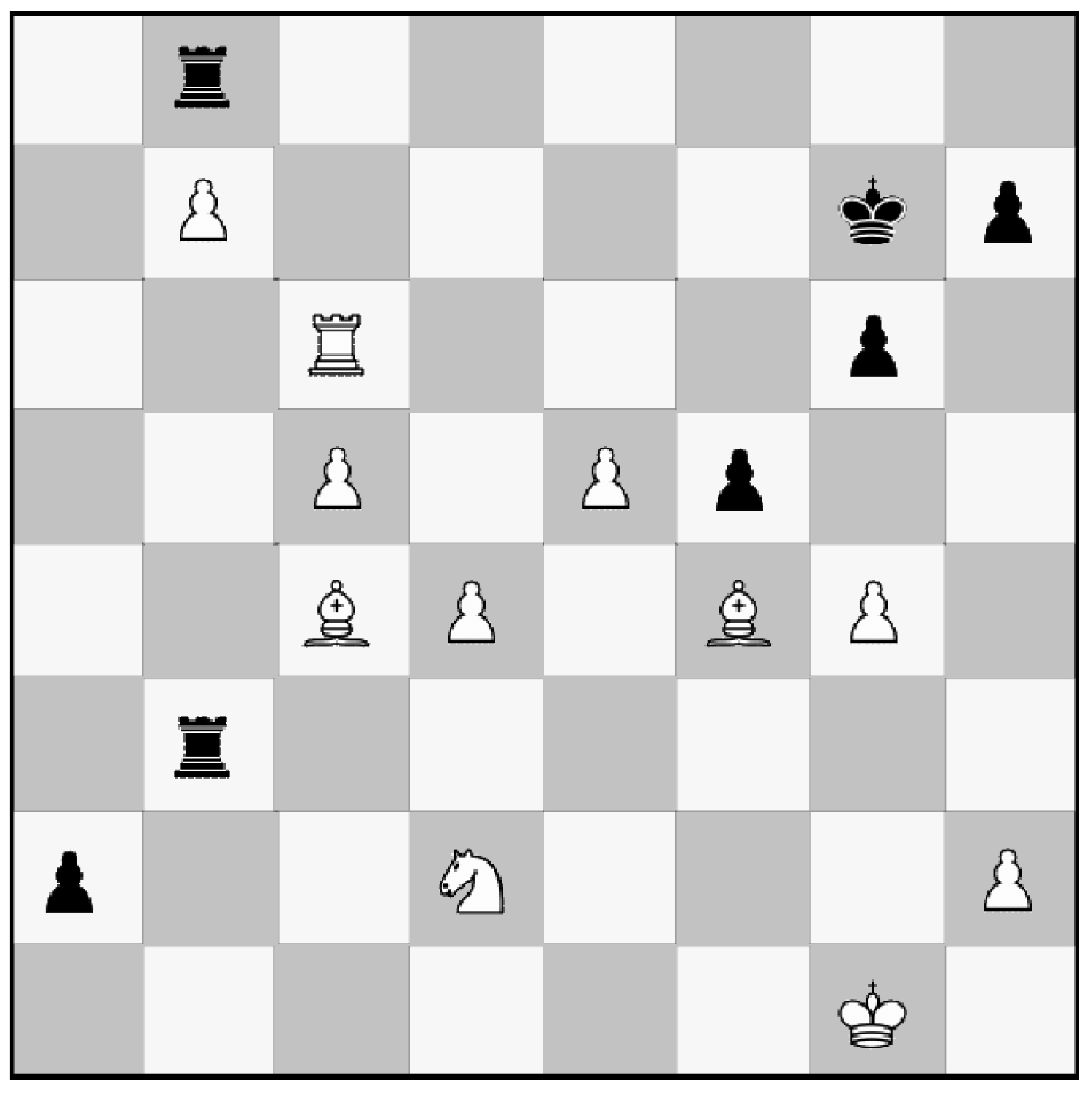
As mentioned above, the results for this study are taken from an experiment that was originally intended to test the memory recall ability of chess players. The stimulus that was presented to chess players for fifteen seconds is shown in Figure 4.

The chess players were approached between rounds of a chess tournament and participation was voluntary. All participants had normal or corrected-to-normal vision. The sample included 28 males and 4 females with average age 31.0 (sd=13.2). One of the male participants could not be calibrated; hence his data was excluded from the subsequent analysis.

Chess expertise was expressed in terms of the ELO rating – a system that was developed by Arpad Elo as a means to measure and rate the average playing ability of chess players (Elo, 1978). The expertise of participants in this study varied from novice (rating 1000) to expert (rating 2400) with an average ELO rating of 1880 (sd=445). Although chess expertise could have an influence on scan paths, it was not considered to impact on fixation identification.

Equipment

Data was captured with a Tobii 1750 eye-tracker. The eye-tracker has a frequency of 50 Hz which means that the PORs were captured and written to the underlying database every 20 ms. The spatial resolution or frame-to-frame variation of the recorded PORs (also referred to as “noise”) of the eye-tracker was about 0.25° (Tobii Technology AB, 2003).

The eye-tracker had a 17” screen and the stimuli were displayed with a resolution of 1024×768 on an eye-screen distance of ±600 mm. Therefore, 1° of visual angle is equivalent to about 33 pixels or 10.5 mm. The individual squares of the chess board spanned about 20 mm (≈2°) while each piece was displayed at about 7×8 mm (<1°).

Calibration was done by displaying five dots at known positions in the same area where the stimulus was displayed.

Determination of benchmark scan paths

As a specific feature of the software tool that was developed for this study, a selection of contiguous PORs can be highlighted manually (see Figure 5 for an example) and the corresponding dots on the stimulus are then displayed in blue (square d3 in the example). Although extremely time consuming, this technique can be used to manually identify fixations, i.e. groups of PORs that belong together both spatially and temporally. In this way, a scan path can be compiled through discretionary selection of a subset of PORs that can be used as benchmark against which the accuracy of fixation detection algorithms can be measured.

Using the tool, each one of the 31 recordings was manually analyzed through visual inspection in order to determine the most probable temporal sequences of PORs to constitute fixations. A rule was implemented that any cluster of PORs should consist of at least six points, i.e. a cluster of PORs should at least represent a minimum duration of 100 ms to be considered a fixation. The scan paths that were identified in this way were regarded as a good approximation of the actual scan paths against which the scan paths identified by the various metrics could be evaluated.

This way of fixation identification is, strictly speaking, also applying a dispersion threshold, but it is not bound to any specific threshold value. The threshold that is applied is variable and based on the discretion of a human observer who has an overview of the entire set of PORs and uses the clustering of PORs as guideline.

Although this way of approximating the actual scan paths could be regarded as subjective and subject to error, the error is believed to be minimal in terms of the number of fixations that were identified (31 participants, 1642 fixations, avg=52.97, sd=8.33).

With reference to Figure 5, it should be noted that fixations on empty squares are not unusual since chess players, especially better players, would look at empty squares to examine possible moves.

Algorithm and metrics

For the purposes of this paper the dispersion-threshold algorithm for fixation identification (I-DT) of Salvucci and Goldberg (2000) was used (Figure 6). This algorithm is quite robust with regard to identified fixation sequences as opposed to other algorithms, e.g. velocitybased algorithms, which may produce inconsistent results at or near threshold values (Salvucci & Goldberg, 2000) or at slow eye movements (Urruty, 2007). Furthermore, the I-DT algorithm is simple and easy to implement and end users have little difficulty comprehending the meaning of the parameters and relating them to published recommendations. The algorithm is also used commonly in analysis tools (Tobii, 2008; Camilli et al., 2008; Gitelman, 2002; Salvucci, 2000). The algorithm is, however, very sensitive to parameter settings (Salvucci & Goldberg, 2000) which necessitates the need to establish the optimum settings.

The algorithm is based on the supposition that fixation points tend to cluster around the same point as a direct consequence of their low velocity. Therefore, PORs that are situated within the dispersion threshold are classified as a fixation. Essentially, the algorithm uses a moving window that spans a minimum number of consecutive data points while inspecting the dispersion of points in the window. If the dispersion is less than a threshold value, the points constitute a fixation. Points are added to the fixation provided that the dispersion is less than the threshold value. When the dispersion is no longer below the threshold a new fixation is identified and the process is repeated until there are no more points.

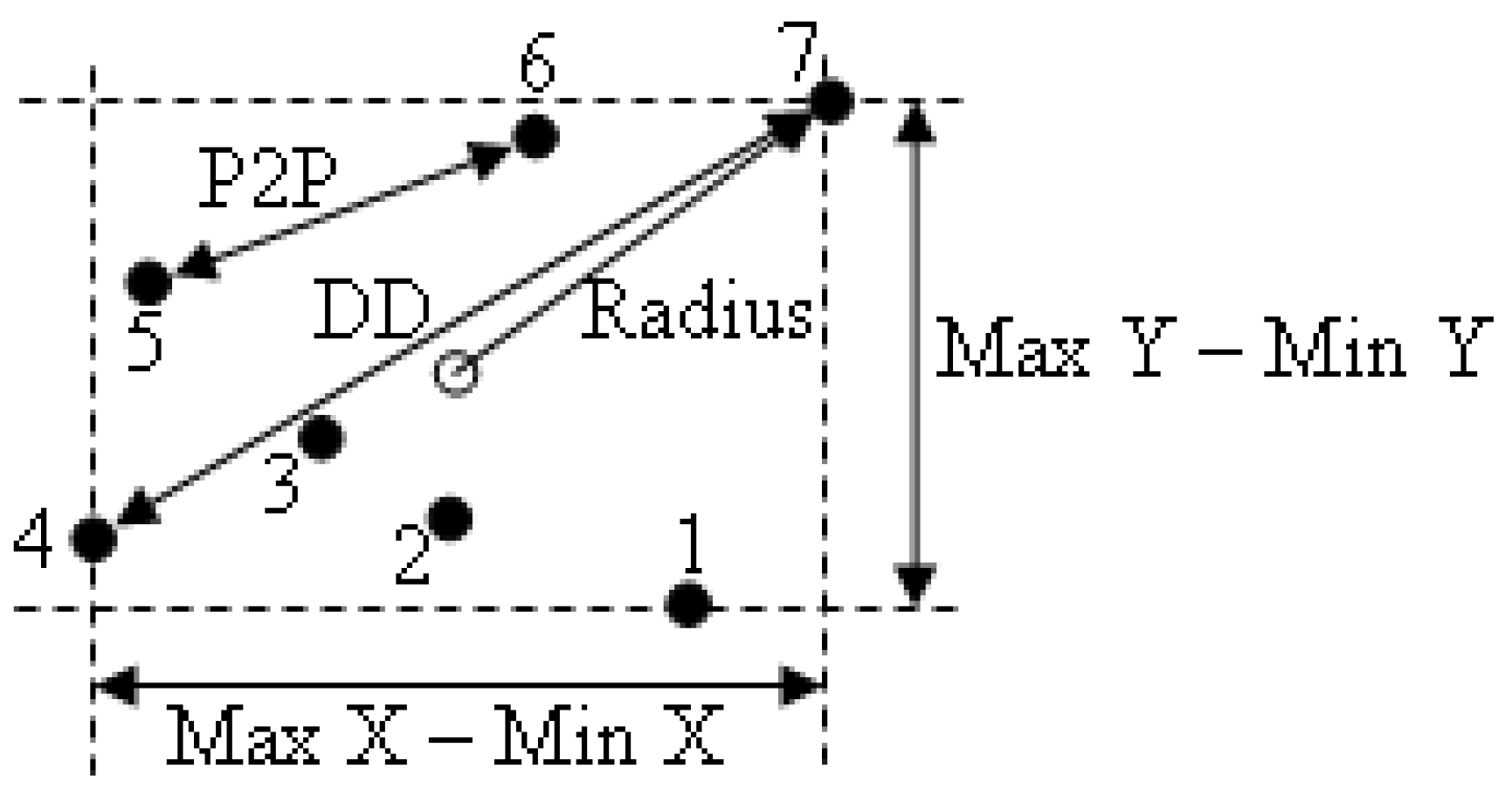
In this study, six metrics were used to measure the dispersion of PORs within a fixation. The metrics were compared with one another in terms of the accuracy of the scan paths that they return and the criticality of the dispersion threshold. The metrics used were:

(i)

the maximum horizontal and vertical distance covered by the PORs in a fixation. i.e. ( (Max X – Min X) + (Max Y – Min Y) ) / 2 ≤ Threshold (Salvucci & Goldberg, 2000) (hereafter referred to as the Salvucci metric),

(ii)

the distance between points in the fixation that are the furthest apart (DD) (Salvucci & Goldberg, 2000),

(iii)

the distance between any two successive points (P2P) (Shic et al., 2008; Spakov & Miniotas, 2007),

(iv)

the distance between points and the centre of the fixation (Radius) (Camilli et al., 2008; Shic et al., 2008),

(v)

the average (Avg) and

(vi)

standard deviation (SD) of the distances of all points from the centre of a fixation (Anliker, 1976; Eyenal, 2001).

Figure 7 shows seven consecutive PORs with the DD, DT, Radius and Salvucci measures of dispersion indicated. The distance between points 4 and 7 is the largest of all the inter-point distances while the distance between points 5 and 6 is the largest of all differences between two consecutive points.

For all metrics of the I-DT algorithm, the duration threshold was set at 100 ms to ensure comparability with the benchmark scan paths. This minimum duration is also in line with Manor and Gordon (2003) who found 100 ms to be a useful and practical balance between the theoretical minimum and maximum limits of fixation duration.

Difference between scan paths

The difference between two scan paths can be expressed in terms of the Levenshtein distance (LD) between them. Specifically, the Levenshtein difference between the benchmark scan path and an estimated scan path as returned by a fixation identification algorithm can be used as indication of the accuracy of fixation identification: The higher the LD, the higher the error in the estimated scan path.

The Levenshtein distance between two character strings is given by the minimum number of operations, defined as insertion, deletion or substitution, needed to transform one string into the other (Levenshtein, 1966). The LD has no cost function and every operation has equal weight. The metric has been applied previously in eye-tracking research in the comparison of scan paths of different participants (West et al., 2006), the scan paths of a participant viewing the same stimuli repeatedly (Foulsham & Underwood, 2008) and the comparison of scan paths returned by an algorithm with a benchmark (Blignaut, 2009). This study follows the latter approach in the sense that scan paths that were returned from different metric / threshold combinations were compared with the benchmark scan path for a specific recording. Other metrics for comparison of scan paths exist, but it was found that they produce similar results (Foulsham & Underwood, 2008) and it was therefore decided that the Levenshtein difference would suffice.

Scan paths were indexed according to the squares on the chess board, a technique that resembles that of Foulsham and Underwood (2008) who divided the stimulus in a 5×5 grid of squares with dimensions 6.4°×4.8° (compared with 2° squares in this study). For example, if the benchmark scan path is d4,c4,c6,f6,g7,g5 and a sequence d4,c4,c6,f6,g7,g5 was reported by a specific metric at a specific threshold, the difference between the sequences would be 2 (one substitution and one deletion). In order to compare the Levenshtein distances of the various recordings, it was expressed as a percentage of the length of the longest sequence. For the above-mentioned example, the LD would thus be 33.3%. The average length of the scan paths in this study was 52.97 (sd=8.33), meaning that if such a scan path contained 5 missing or misplaced fixations or fixations that were wrongly inserted, the LD would be 9.4%.

The optimum threshold for a specific metric would be a value where the Levenshtein distance between the estimated scan path and the benchmark scan path is a minimum. The best metric would be the one that returns the lowest minimum Levenshtein distance.

It is possible that an identified fixation might consist of a different subset of PORs than the corresponding fixation in the benchmark scan path, therefore having different coordinates for their centres. These fixation centres could be in the same or adjacent squares in the grid, meaning that the displacement can either be reflected in the Levenshtein distance between the scan paths or not. Inspection revealed that this uncertainty occurs only for fixations that are located right on the edges of squares and when a POR that is quite some distance from the centre of the fixation falls in the adjacent square. The frequency of occurrence of this scenario is, however, very low.

Results

The effect of threshold and individual differences on the accuracy of scan paths

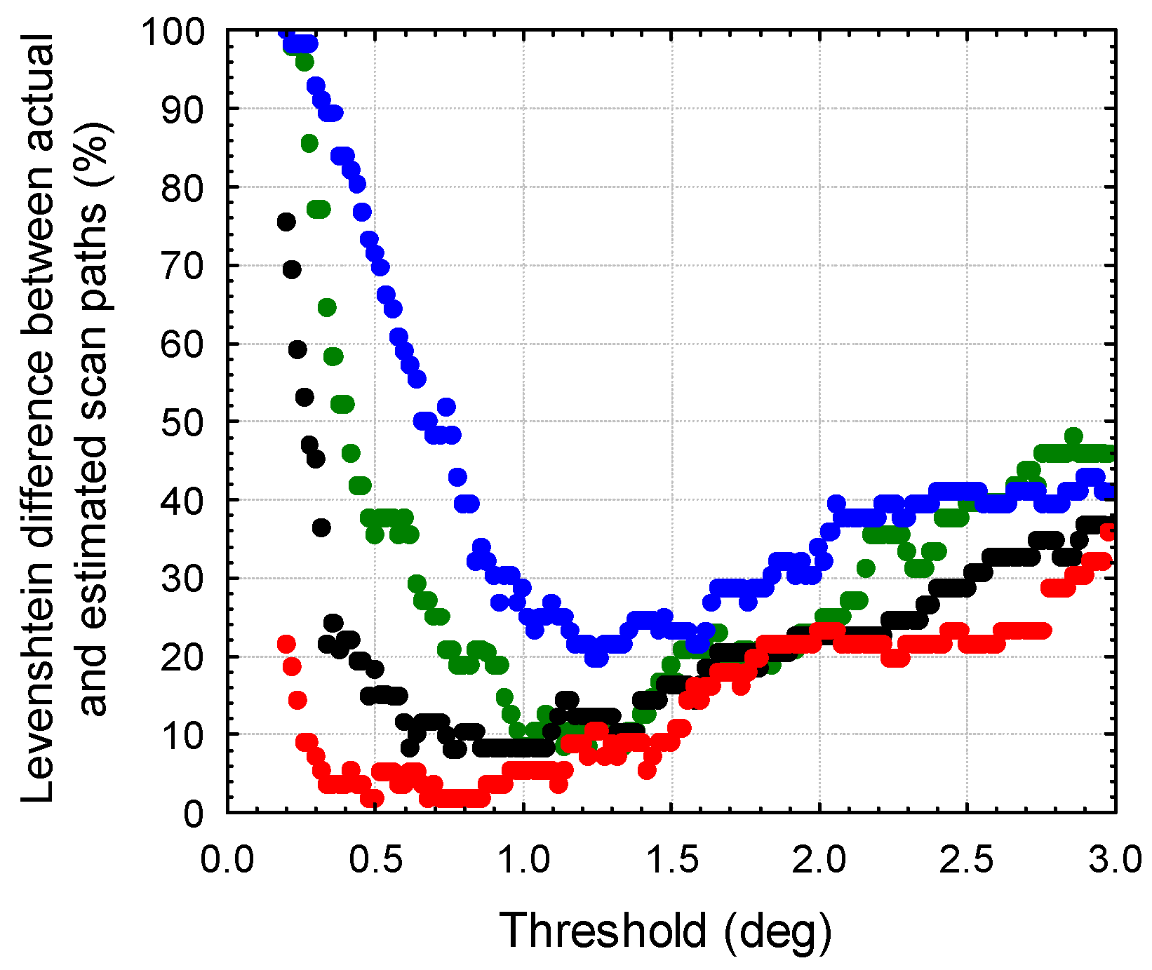
It was found that the accuracy with which scan paths can be identified differs from one individual to the other as well as with regard to the threshold value that is used. Also, the minimum Levenshtein difference is different for different individuals and these minima occur at different thresholds.

As an illustration, Figure 8 shows the Levenshtein distance (LD) against the threshold value for four participant recordings after application of the Radius metric for fixation identification. Each data point represents the LD for a specific participant at the respective threshold.

Comparison of metrics and identification of an optimum per-metric threshold

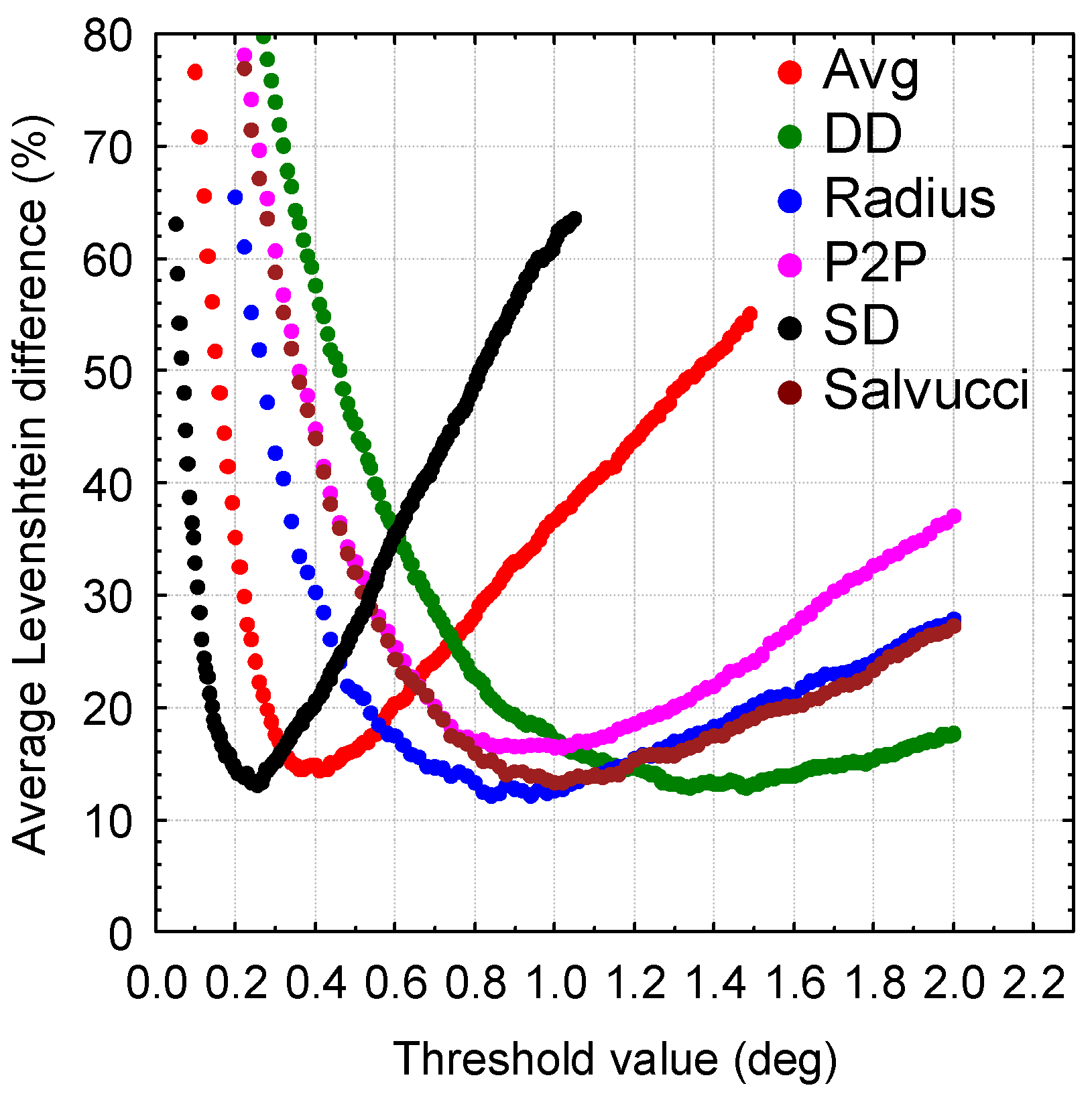
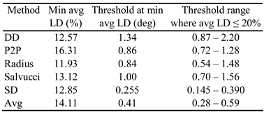
Instead of a separate data point for each recording as in Figure 8, Figure 9 shows the average LD of all recordings against threshold. Curves for all metrics are combined on the same graph. The minimum of the average LDs and corresponding threshold values are given in

Table 1. Minimum average Levenshtein distance and corresponding threshold value.

along with a range of threshold values where the LD is below 20%.

The Radius metric has the lowest minimum average Levenshtein distance (11.93%). The threshold at minimum LD (0.84°) agrees with the recommendation by Blignaut (2009) and it is also clear that, at least for the type of stimuli that were used in this study, the 0.5° threshold that is sometimes recommended (Salvucci & Goldberg, 2000; Hornof & Halverson, 2002) is too low. In fact, looking at the slope of the various portions of the curves in Figure 11, it is clear that it is less critical to err with a threshold that is too high than having it too low.

The DD metric also has an LD which is quite low (12.57%) but it has a wider range of threshold values where LD is less than 20%. The P2P metric has a much higher minimum LD (16.35%) with a narrow range of acceptable threshold values. The Avg and SD metrics have extremely narrow ranges of acceptable threshold values. The Avg and SD metrics have extremely narrow ranges of acceptable threshold values. Taking all this into account, it seems that the DD and Radius are the preferred metrics for the I-DT algorithm.

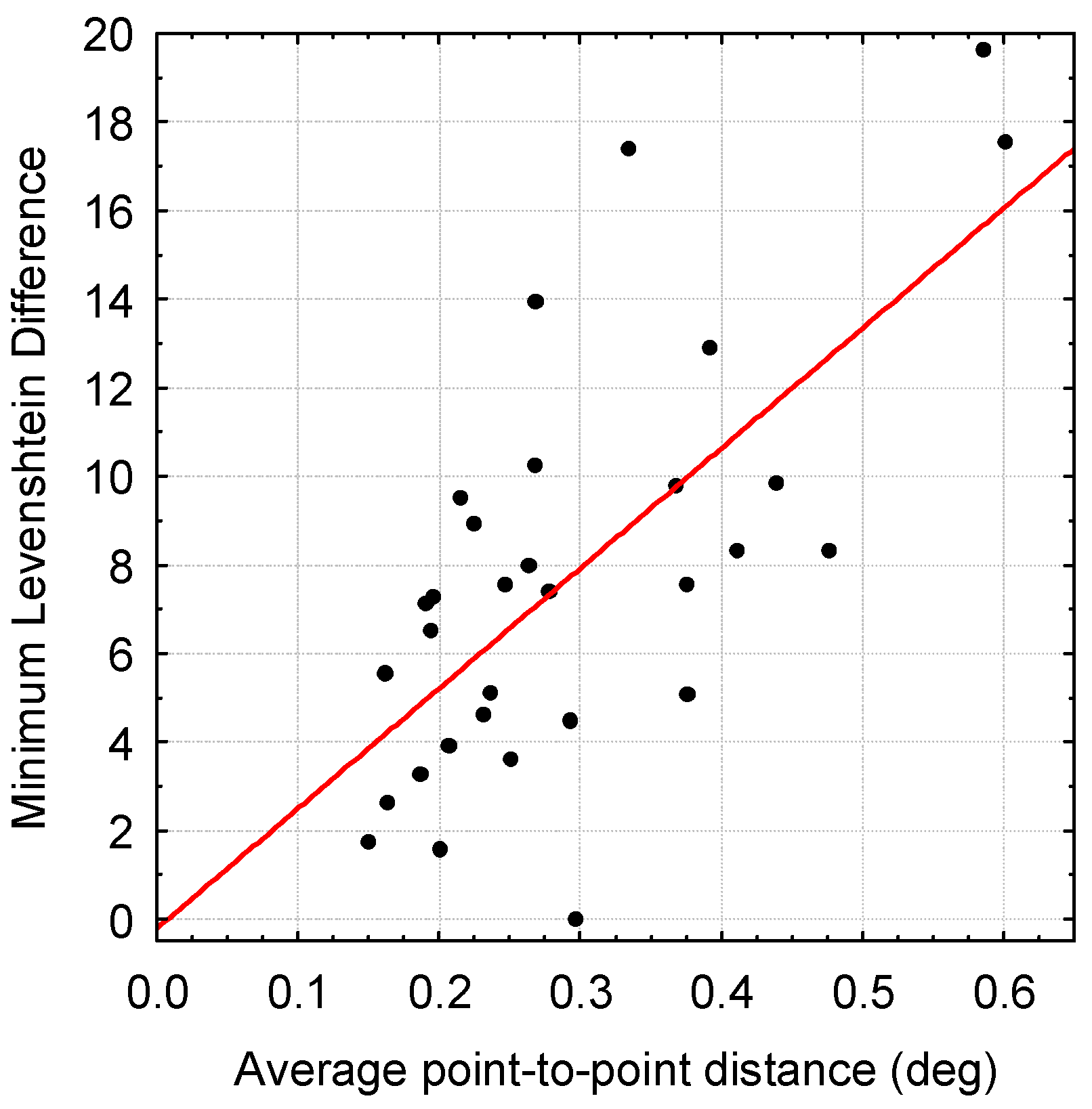
The effect of fixational eye movements on the accuracy of scan paths

Figure 10 shows a graph with a linear regression line of the minimum LD against average point-to-point distance for the 31 individual participants after application of the Radius metric for fixation identification.

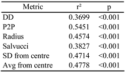
The significance of the linear regressions for all metrics is given in

Table 2. Significance of linear regressions of minimum Levenshtein difference against average point-to-point distance per participant for each of the metrics.

. Since r² is significant for all the metrics, the hypothesis as stated above can be confirmed: the differences amongst people with regard to fixational eye movements have an effect on the accuracy with which fixations are identified from raw gaze data. The less stable the eye gaze, the less accurate the fixation identification is.

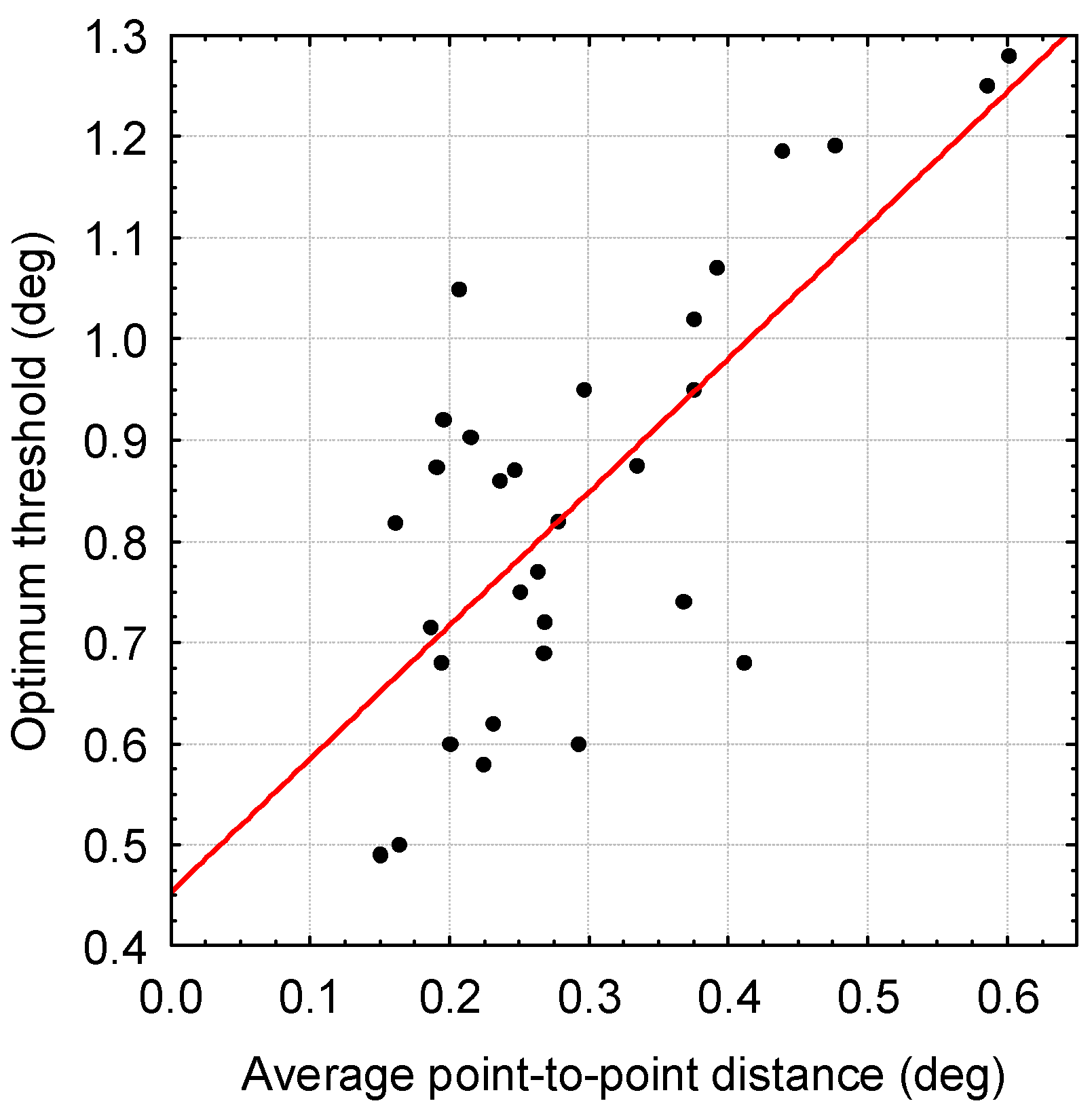
The effect of fixational eye movements on optimum threshold

Figure 11 shows a graph with a linear regression line of the optimum threshold (the threshold where LD is a minimum for the specific participant) against the average point-to-point distance of PORs within fixations for the Radius metric for each individual participant. The significance of the linear regressions for all metrics is given in

Table 3. Significance of linear regressions of optimum threshold against average point-to-point distance per participant recording for each of the metrics.

.

There is a significant (p<0.001) positive correlation between the optimum threshold values for each of the metrics and the average point-to-point distance within fixations for individual participants. With regard to the hypothesis stated above, it is thus confirmed that the differences amongst people with regard to fixational eye movement also have an effect on the optimum dispersion threshold for the various metrics. The less stable the eye gaze, the higher the optimum dispersion threshold that should be used in the fixation identification algorithm.

Applicability of a common per-metric threshold to all participants

Table 4. Average Levenshtein distances (sd in brackets) between the benchmark scan path and the scan paths as returned by the various metrics and threshold settings.

* 1: A different threshold for each participant, i.e. the threshold at which the LD is a minimum for the respective participant 2: The generic optimum for a specific metric as given in Table 3.

shows the average and standard deviations of the average Levenshtein distances that were obtained with the two possible sets of threshold settings along with the results of an analysis of variance. For all the metrics, the average LD based on the optimum threshold per participant is significantly (p<0.05) lower than the average LD based on the generic optimum threshold for the specific metric. Therefore, it is clear that a generic threshold for each metric is not optimal for all participants. However, since it is not practical to have a separate threshold for each participant and because it is not easy to determine the optimum threshold for each participant beforehand, this is the only viable solution.

Fortunately, if the threshold is chosen with care, the results can still be acceptable with an average error of less than 20%.

Summary and Conclusions

Cognitive processing of a visual stimulus occurs during fixations – a period of time in which the eye remains relatively still. During fixations, the eye is subject to different types of low velocity movements, such as tremors, drifts and microsaccades. The challenge to identify fixations from raw gaze data is, therefore, subject to two basic sources of error:

(i) The amount of fixational eye movement. It was hypothesized that individuals differ from one another with regard to the amount of fixational eye movement and that these movements have an effect on the optimum threshold setting for a dispersion-based algorithm as well as the accuracy with which fixations can be identified from raw gaze data. An inevitable consequence of this hypothesis is that a common dispersion threshold is not necessarily optimal for all participants.

(ii) The algorithm used for fixation identification. Depending on the nature of the algorithm, the choices made and parameters chosen have an effect on the accuracy of the scan paths that are identified. This paper focused on the dispersion threshold algorithm and the various metrics for dispersion as described in Salvucci and Goldberg (2000). The nature of the various metrics for this algorithm is such that each metric has a different optimum threshold (Table 1).

A graph of the average Levenshtein difference of all participant recordings against threshold was used to determine a generic optimum threshold value for each metric (Figure 9). Visual inspection of this graph revealed that the Radius and distance dispersion (DD) metrics return the most accurate scan paths while the correct threshold settings are not as crucial as for the other metrics.

The average point-to point distance of PORs within fixations was used as indicator of fixational eye movement of a specific participant recording. Using this indicator, it was confirmed statistically that individuals differ from one another with regard to the amount of fixational eye movement during fixations (Figure 3).

A software tool was developed to identify fixations from raw gaze data. Six metrics of dispersion were applied one after the other. For each combination of participant and metric, a scan path was generated for each threshold value in a range of values between 0.2° and 3.0° at regular intervals. The accuracy of these scan paths was expressed in terms of the number of edit operations that would be necessary to transform them to the respective benchmark scan paths (the so-called Levenshtein difference). The optimum threshold for each recording was considered to be the dispersion value where the Levenshtein difference is a minimum.

The hypothesis as stated was found to hold in all respects. A regression analysis of error in the scan path (minimum LD) against fixational eye movement proved that the latter has an effect on the accuracy with which fixations are identified from raw gaze data (Table 2). The less stable the gaze is, the less accurate the fixation identification is. This holds for all metrics of the dispersion algorithm.

A regression analysis of the threshold at which the minimum LD was attained against fixational eye movement also proved that fixational eye movements have an effect on the optimum dispersion threshold for each one of the metrics (Table 3). The less stable the gaze, the higher the optimum dispersion threshold that should be used in the fixation identification algorithm.

The average Levenshtein difference of all participant recordings at the generic per-metric optimum threshold was significantly higher than the average Levenshtein difference if the optimum threshold as applicable for each individual was applied (Table 4). Unfortunately, it is generally not feasible to have a separate threshold for each participant, essentially because it is difficult to determine what the unique threshold should be. Therefore, it is of utmost importance that the generic threshold should be chosen with care, especially if the participants are not homogeneous with regard to gaze stability. Homogeneity in this regard can be improved by ensuring that nobody has health problems that can affect gaze stability such as Alzheimer’s disease or ADHD and that the participants are of the same age group as far as possible.

It is acknowledged that the errors induced by the subjective method to approximate the actual scan paths and the uncertainty with regard to the centre coordinates of fixations on the edges of a square could have had minor influences on the numeric values of the Levenshtein differences and the F-values for the respective Anova tests. It is believed, however, that the influences are not large enough to impact on the significance of the F-values. This means that although the magnitude of the effects might be uncertain, the general trends of the above-mentioned findings still hold.

Future research

Although the result that PORs that are further apart require a higher threshold in order to aggregate them into fixations could have been expected, it is a principle that has been widely neglected by commercial eye-tracking applications to date. Currently, most commercial eyetracking applications recommend the same threshold setting for all participants and do not provide a way of analysing the amount of fixational eye movements or distinguishing between participants.

This paper now formalizes the principle that individuals differ with regard to the density of PORs within a fixation and provides motivation for further research on ways to adapt the threshold to individual differences easily and dynamically. It is suggested that commercial eye-tracking systems should provide for some kind of pre-test (possibly as part of calibration) in order to recommend a personalised threshold setting for individual participants.

The technique that was used in this paper to identify benchmark scan paths against which the accuracy of the fixation detection algorithm was measured, was subjective in the sense that it relied on the discretion of a human observer to identify clusters of PORs that designate a fixation. A future experiment could be devised in which the participants are instructed to specifically look at certain elements of a stimulus so that the exact positions of fixations are known.

The effect of the uncertainty with regard to the centre coordinates of fixations on the edges of a square could be examined by studying the same data set on grids that vary in size and/or position.