Probabilistic Approach to Robust Wearable Gaze Tracking

Abstract

This paper presents a method for computing the gaze point using camera data captured with a wearable gaze tracking device. The method utilizes a physical model of the human eye, ad-vanced Bayesian computer vision algorithms, and Kalman filtering, resulting in high accuracy and low noise. Our C++ implementation can process camera streams with 30 frames per second in realtime. The performance of the system is validated in an exhaustive experimental setup with 19 participants, using a self-made device. Due to the used eye model and binocular cam-eras, the system is accurate for all distances and invariant to device movement. We also test our system against a best-in-class commercial device which is outperformed for spatial accuracy and precision. The software and hardware instructions as well as the experimental data are pub-lished as open source.

1. Introduction

Gaze tracking is finally evolving from studies that are mainly performed in controlled laboratory environments and desktop trackers to field studies running on wearable hardware. These kind of mobile systems are applicable to actual operational environments and workplaces, e.g., walking, driving, operating machinery, and interacting with the environment and other people. Mostly due to the novelty and high price of the mobile gaze tracking tech-nology, application potential remains, for the most part, unutilized.

Current commercial systems for wearable gaze track-ers offer working solutions for industrial and research cus-tomers but are expensive and hide the implementation of their tracking hardware and algorithms behind proprietary solutions. This limits their accessibility, areas of applica-tion, and the scale and scalability of gaze tracking and in-hibits their further development, integration, customiza-tion, and adaptation by the expert community of gaze tracking users and researchers. Also, the reported perfor-mance metrics are hard to cross-evaluate between systems as they are typically reported for “optimal" tracking con-ditions and well-performing subjects. Therefore, while commercial systems can supply high-performing solu-tions, there is still a need for a low-cost alternative that opens up the further development of gaze tracking meth-ods and algorithms. Enabling the larger user community to build their own trackers opens the playground for innovations, novel approaches, and more rapid development cy-cles. Computationally, the big challenges in mobile gaze tracking include changing lighting conditions and move-ment of the device in relation to the eyes of the users.

In this paper, we present the algorithmic basis of our current open-source gaze tracker. The system provides a robust, probabilistic approach for realtime gaze tracking, especially for use with a mobile frame-like system, alt-hough the presented algorithms should also work for re-mote settings. The algorithms are based on advanced Bayesian modeling while utilizing a physical eye model. The system has proven very robust against dynamic changes in external lighting and possible movement of the gaze tracking frame in relation to the eyes of the user.

Our hardware implementation is built from off-the-shelf sub-miniature USB cameras and optical filters, a sim-ple custom printed circuit board, and a 3D printed frame. Apart from a standard laptop computer for running the software, the total cost for the system is ca. 700 euros of which 80 % is dictated by the cameras. The software and the design of the circuit board and frame are released as open source under a permissive license.

The temporal requirement of realtime systems (i.e., processing the video frames within the frame rate of the cameras) poses a challenge. Conventional USB-cameras capture 20–30 frames per second which our software im-plementation is able to handle. However, due to the com-plexity of the methods, using cameras with higher frame rates (such as 100 fps) may call for special solutions such as hardware acceleration or parameter optimization.

In addition to performance metrics, we provide a com-parison to a best-in-class commercial system (SMI Eye-tracking Glasses with iView 2.1 recording software and BeGaze 3.5 analyzing software) in the same setting. Based on our experiments with 19 participants, the commercial system is outperformed for spatial accuracy and precision. The recorded data is published openly, too.

Summarizing, the contributions of this paper are:

• A complete probabilistic gaze tracking model and its full implementation.
• Exhaustive evaluation of the performance of our system and publication of the recorded data openly for others to test.
• Validation of the performance of the commer-cial SMI gaze tracking glasses system.
• C++ software implementation and hardware instructions published as open source.

1.1. Related Work

The large majority of gaze tracking research thus far has been performed in desktop environments using remote trackers, with the eye tracker and light sources integrated to the desktop environment and calibrated for a planar computer monitor. A number of wearable gaze trackers, both commercial and open-source, are also available. These allow the user to move around more freely and track gaze outside a single screen space. While the basic track-ing methodology utilized is largely similar – tracking op-tical features of the eye – there is large variation in tech-nical details, performance, and robustness between the systems. A wide survey of gaze tracking methodology is presented by Hansen and Ji (2010). Hayhoe and Ballard (2005) offer a more mobile-centric review and Evans et al. (2012) focus on outdoor gaze tracking and some of the complexities inherent in taking gaze tracking out of the lab.

The most typical solution in video-based gaze tracking is to track the pupil and usually one corneal reflection (CR) from a light source to offer rudimentary compensation for camera movement relative to the eye. These methods use a multi-point calibration on a fixed distance, mapping changes in pupil and CR positions to interpolated gaze points (Duchowski 2003). A more sophisticated solution utilizing a physical model of the eye was suggested in the desktop genre (Shih and Liu 2004; Guestrin and Eizenman 2006; Hennessey et al., 2006). These require at least two light sources and the respective CRs for solving the geo-metrical equations involved and also some sort of user cal-ibration to compensate for the personal eye parameters. User calibration is usually lighter than with mapping meth-ods; Chen and Ji (2015) even proposed a calibration-free model based method.

The mobile setting poses more challenges than the desktop setting due to, e.g., changes in lighting and device orientation. As an added complication, the gaze distance varies when the user freely navigates her environment which leads to variable parallax error when gazing at dif-ferent distances as the eyes and the camera, imaging user’s view, are not co-axial (Mardanbegi and Hansen 2012). The gaze distance can be approximated with at least three so-lutions: use a fixed distance, use metric information about the environment based on visual (fiducial) markers, or em-ploy binocular trackers (i.e, having eye cameras for both eyes) and produce an estimate for gaze distance using the convergence of both eyes’ gaze vectors that can be com-puted with the physical model.

Commercial systems offer proprietary solutions to gaze tracking. Notable examples include Tobii Pro Glasses (http://www.tobiipro.com/product-listing/tobii-pro- glasses-2/), Ergoneers Dikablis system (http://www.er-goneers.com/en/hardware/eye-tracking/eye-tracking-head-mounted/), and SMI Gaze tracking glasses (http://www.eyetracking-glasses.com/), the latter used here as a reference for evaluating performance. A consid-erable number of open solutions for gaze tracking have also been suggested. Earlier mobile open source gaze tracker systems include the openEyes system (Li, Bab-cock, and Parkhurst 2006) that introduced the popular Starburst algorithm for detecting eye features; the ITU Gaze Tracker system (San Agustin et al. 2010) that aims at providing a low-cost alternative to commercial gaze track-ers; and the Haytham (Hales, Rozado, and Mardanbegi 2013), developed more toward direct gaze interaction in real environments. Pupil labs offer both commercial and open-source systems (Kassner, Patera, and Bulling 2014) and Ryan, Duchowski, and Birchfield (2008) aimed at a tracker operating under visible light conditions.

Here, we extend the physical eye model approach in-troduced by Hennessey, Noureddin, and Lawrence (2006). We utilize Bayesian methodology to provide a robust method for accurate gaze tracking in real time. Work to-ward the current system has been described by Lukander et al. (2013) which used a similar approach but with a dif-ferent optical setup, monocular tracking, and a heuristic feature tracking solution; Toivanen and Lukander (2015) who presented probabilistic ideas for tracking the eye fea-tures; and Toivanen (2016) who introduced a preliminary version of the Kalman filter for stabilizing the result.

2. Proposed method

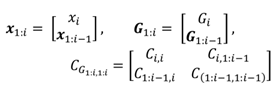
Before going into more details with the method, let us give some definitions. The method is supposed to be used with a wearable gaze tracking system, a.k.a., gaze tracking glasses. The glasses contain one or two eye cameras that point towards eyes. There is also a scene camera pointing towards user’s scene. The glasses contain LED light sources, attached to the frame of the glasses. Each LED causes a reflection on the eye surface as seen by the eye camera, called a glint. The mutual configuration of the glints is specific to the placement of the LEDs in the glasses although this configuration changes according to the shape of the eye and pose and distance of the glasses with respect to the eye. The (average) mutual configura-tion, or shape, of the glints is called a glint grid. The num-ber of LEDs is denoted with NL and the glint grid contains thus NL glints. The captured eye image is generally de-noted with $ℐ$ throughout the paper but its specific form (in terms of preprocessing) depends on the context and is clar-ified accordingly. An example of gaze tracking glasses with six infrared (IR) LEDs is shown in Figure 11, and an example of an eye image, captured with it, is given in Fig- ure 2. For the sake of clarity, throughout the paper the no-tation for matrices and vectors is not bolded except when being multivariate.

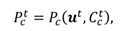
The objective of the presented method is to estimate the three-dimensional point-of-gaze (POG) and its 2D pro-jection in the image plane of the scene camera, utilizing a simplified eye model and knowledge about the configura-tion of the cameras and LEDs in relation to each other. The identified 3D POG can also be projected to other reference coordinate systems, such as one based on fiducial markers detected in the scene image, but here we concentrate on the case of scene video.

Mobile gaze tracking sets additional requirements for the performance as compared to desktop gaze trackers: dy-namic lighting conditions require better tolerance for changing luminosity and extra reflections and tracking the eyes of a moving subject calls for robustness against pos-sible movement of the device in relation to the tracked eyes. This necessitates using more LEDs than what is typ-ically used in desktop trackers which then again increases the probability of some glints being non-visible. Also, in wearable systems the LEDs must be located at the very edge of the view to minimize their disturbance whereas in remote systems the LEDs can be located near center of the field of view. In addition, with the desktop gaze trackers the gaze distance is approximately constant, as opposed to mobile tracking. While a simpler mapping-based approach may be sufficient for desktop trackers, the variable nature of mobile tracking is better handled with a model-based approach.

2.1. System overview

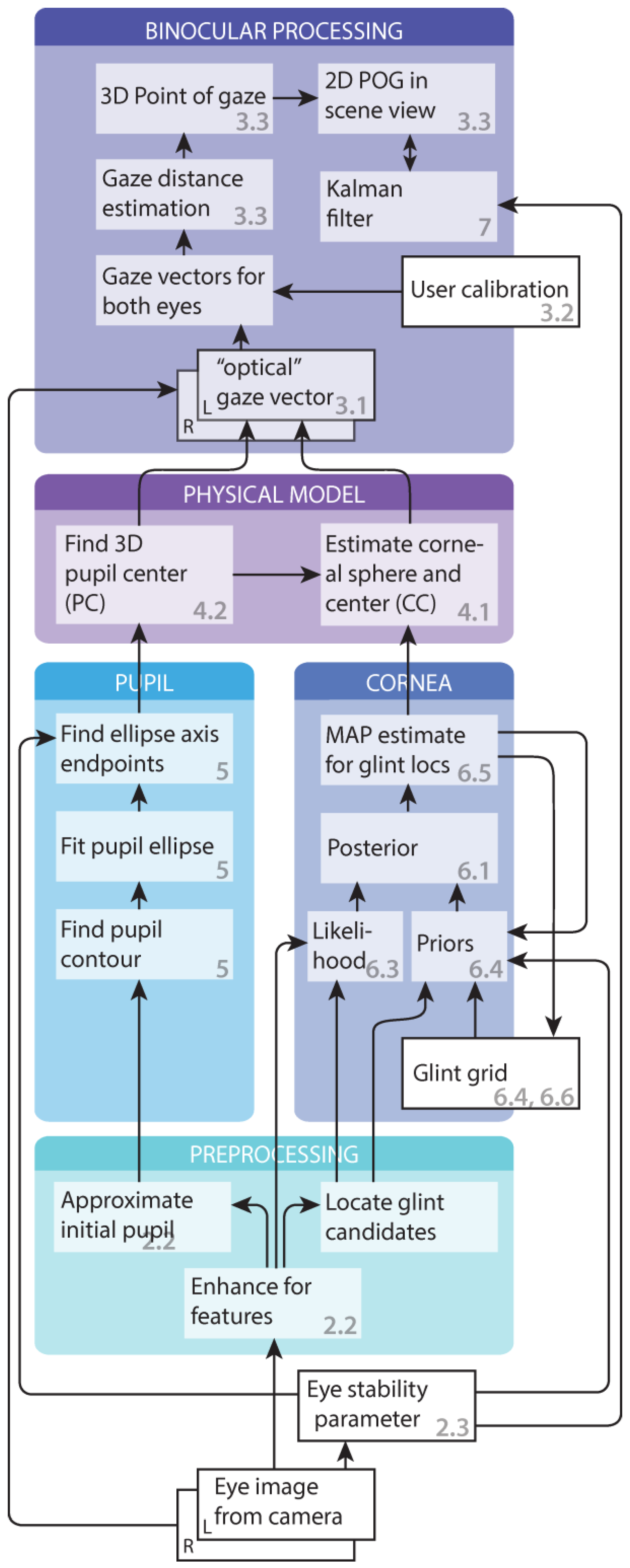
Figure 1 presents a flowchart of the processing pipeline for video frames. The frames grabbed from the cameras are first preprocessed for finding the pupils and the corneal features. These are used in computing the 3D cornea cen-ters and pupil locations of the physical eye model. From these, the gaze vectors, and ultimately the gaze point in the scene video can be computed utilizing user calibration in-formation. To stabilize the results, the gaze point can fur-ther be Kalman filtered. Here, the focus is on supplying gaze location and path. However, fixations and saccades can be roughly estimated using the eye stability parameter which estimates how stable the eye has been during the latest video frames. In addition, the frames where eye fea-tures cannot be detected can be assigned as blinks.

For the utilized physical eye model (“physical model" block in the flowchart) we use the model presented by Hennessey (2006); Shih and Liu (2004). The main contri-bution of this paper arises from applying the method to wearable gaze tracking and the methodology in the other blocks in Figure 1. Probably the greatest contributions are in the computer vision related tasks (“pupil" and “cornea" blocks) and in the Kalman filter. The glint grid is generally more difficult to locate than the pupil because there may be additional distracting reflections in the image and some of the glints may not always be visible. Therefore, we use a simpler detection scheme for pupil and a more advanced Bayesian tracking model for glints. The Bayesian ap-proach allows neatly combining the expectations about the appearance of the glints and their mutual configuration. In addition, glints are likely to depend on their locations in the previous image; for most of the time, eyes fixate on the same point and the glints are stationary. With the Bayesian tracking framework, we can utilize this information in a sophisticated manner.

The cameras are modeled as pinhole cameras. The in-trinsic and extrinsic parameters are estimated using the conventional calibration routines (Zhang, 2000).

2.2. Preprocessing the eye image and ap-proximating the pupil center

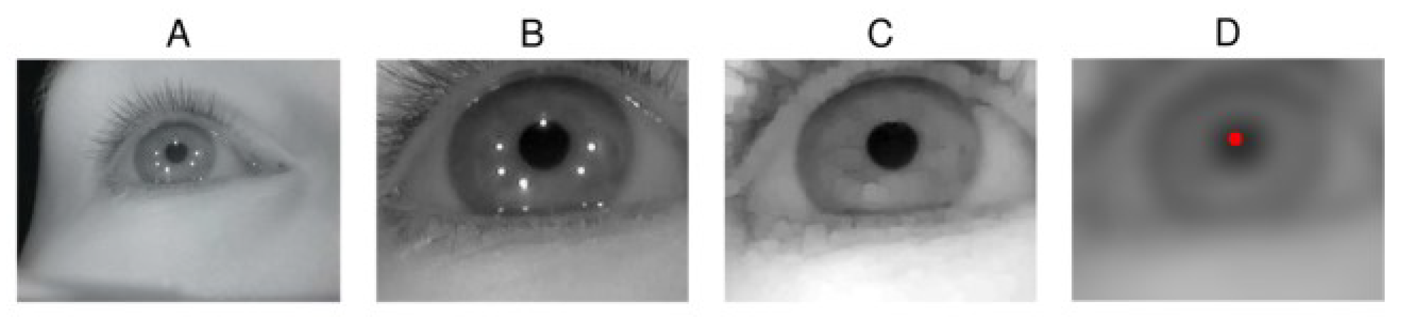
Figure 2A illustrates an eye camera image captured while wearing the glasses that are shown in Figure 11. The pupil and all the LED reflections (i.e., glints) are clearly visible. The eye images are preprocessed to decrease the image size by cropping away useless parts and color chan-nels in the image in order to accelerate the computations, and to remove noise and enhance certain image features. Images B, C, and D of Figure 2 shows some preprocessing stages.

The captured IR image is practically monochromatic so it is first converted to a grayscale image. Because the eye can be assumed to stay at a relatively fixed position in the image, the image is cropped around the assumed eye location, using a constant cropping area (B). For finding the initial approximation for the pupil, the cropped image is morphologically opened to remove the glints (C). Then, an approximate pupil center is located in order to further crop the image. For estimating the pupil center, the opened image is filtered by convolving it with a circular kernel whose radius approximately equals the expected radius of a pupil in the eye images; this removes dark spots that are smaller than the pupil so that after the filtering the pupil center would be the darkest pixel, which is considered to be the approximate pupil center (D). Despite the relative simplicity, this approximate pupil center detection per-forms well. In our experiments, only very dark and thick make-up in the eyelashes caused the pupil center to be misdetected in the eyelash area.

Different preprocessed stages are used in different parts of the algorithms: the eye stability estimator uses the filtered image (Figure 2D); the pupil localization uses the opened image (C) and estimated pupil center; and the glint localization uses the cropped and opened images (B and C) together with the estimated pupil center.

2.3. Estimating stability in eye image

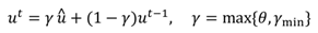
We use information about how stable the eye image has been during the most recent k + 1 previous video frames later in Sections 5, 6.4, and 7. To quantify this stability measure we use a simple scaled and smoothed estimator of an average change in the eye images that gives a value θ ∈ [0,1] which is close to unity if there have been large changes in recent frames and close to zero if the eye seems to have been relatively stable.

More formally, given parameters αm, λm > 0, w > 0, and the size of the smoothing window k + 1, we define the stability θ^t at time instance t as

(1)

where S^t = max{S^t−k, . . . , S^t} is the maximum value of the previous k + 1 sigmoid values, defined as

(2)

where m^t is a pixel-wise L₂ norm between subsequent frames:

(3)

where $ℐ$^t is the observed (cropped, opened, and filtered) eye image at time t (see Figure 2D for an example) and De is the number of pixels in the image. The parameter θ^t is estimated for the right eye image only since the eyes nor-mally move in synchrony. The parameter values that we use in our experiments are presented in Table 2.

3. Physical eye model

The following section details the basic principles of computing the POG with the physical model.

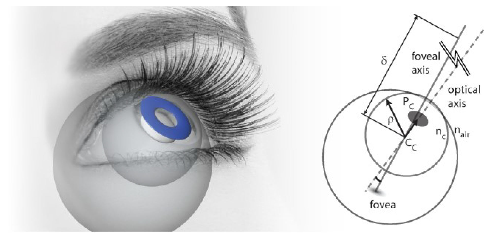
3.1. Gaze point computation

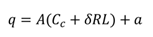
Figure 3 illustrates the used (simplified) physical model of the human eye. The axis that traverses the 3D centers of the pupil (Pc ) and the corneal sphere (Cc) is called the optical axis. The corresponding unit vector is called the optical vector, denoted as L. The actual gaze vector that we are interested in traverses (approximately) through the cornea center and fovea which is the spot on the retina with the highest density of photoreceptors. The optical and gaze vectors are not parallel. Hence, the gaze point gp is computed as

(4)

where R is a matrix that rotates the optical vector to coin-cide with the gaze vector and δ is the viewing distance be-tween Cc and the gaze point. Note that (4) applies for both eyes, each with its own gaze point. If two eye cameras are in use, the gaze distance δ can be estimated (see Subsec-tion 3.3).

3.2. User calibration

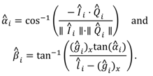
The rotation matrix R is a person-dependent constant as the location of fovea, and thus the angular difference between the optical and foveal axes vary between individ-uals. This section describes how to estimate R; this proce-dure is called user calibration.

Let us assume that we know the transformation be-tween the coordinate systems of each camera (both eye cameras and the scene camera). The 3D points Pc and Cc are originally defined in the coordinate system of the cor-responding eye camera. For computing the gaze point, the 3D points in the left eye camera coordinates are trans-formed to the right eye camera coordinates. Then we can transform both eye’s gaze point to scene camera coordi-nates. Let A and a denote the rotation and translation parts of this transformation. The gaze point in the scene camera, q, can thus be computed as

(5)

where Cc, δ, R, and L “belong" to either the left or the right eye.

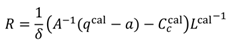
In the user calibration procedure, the user fixates sev-eral points which are a fixed distance δ away from the user and which are simultaneously annotated in the scene cam-era video. For each annotation, the cornea centers and gaze vectors are extracted as well as the annotated 3D target values which can be estimated using the camera calibration information and the fixed distance to the calibration target. The calibration routine with Nc samples results thus in a collection of points and vectors {qⁱ, Cⁱ, Lⁱ, i = 1,2, . . . , Nc} which we denote with q^cal, C^cal, and L^cal.

Eq. (5) should hold for each sample as well as possible so R is estimated in a least-squares sense as

(6)

where the inverse of L^cal can be solved with, e.g., pseudoinverse, as long as Nc ≥ 3. Note that the viewing distance δ must be set to the real distance between the viewer and target, which distance is also used for compu-ting the target points q^cal – this should lead to negligible error as it can safely be assumed that the distance from the scene camera origin to the target approximately equals the distance from the cornea center to the target because the target distance is much larger than the distance between the scene camera and the eye. Calibration sets C^cal and L^cal naturally differ between the eyes, resulting in separate cal-ibration matrices for both eyes, R^L and R^R.

The matrix R is, however, not strictly a rotation matrix but a general transformation matrix. This transformation can be thought of as dealing with all other kinds of (more or less systematic) inaccuracies present, apart from the an-gle between gaze vector and optical vector. Errors may stem from the following factors: some user-dependent eye parameters are set to constant population averages, the physical eye model is over-simplified, the used pinhole camera model is only approximate (while calibrated), the estimated transformation matrices between LEDs and cameras are imperfect, and there may be inaccuracies in the estimated corneal and pupil centers. Because R is not a rotation matrix, its determinant is not unity and it is not orthogonal. Therefore, the unit of δ is, strictly speaking, not metric but the norm of RL which might slightly deviate from unity and may thus attribute a minor error into the estimation (6). Finally, it should be noted that the user cal-ibration needs to be done only once for each user after which the same calibration information can be used repeat-edly.

3.3. Computing the binocular POG

The gaze point can be computed using Eq. (5) for both eyes separately and taking the middle point:

(7)

where superscripts ^L and ^R refer to left and right eye. We are left with estimating the gaze distances δ^L and δ^R for which we present two different methods. When gazing at a point, the left and right gaze vectors of the viewer are directed (approximately) to the same gaze point. Actually, due to possible fixation disparity there might be a slight mismatch between the gaze vectors (Jainta et al. 2015).

We can thus minimize the squared difference between the left and right gaze points (see Eq. (4)) for solving the left and right gaze distances δ^L and δ^R. We get equations (8) and (9), where g = RL/∥ RL ∥ is the normalized gaze vector.

(8)

(9)

When gazing at a long distance, the gaze vectors are nearly parallel and slight inaccuracy in the estimation may cause the gaze vectors to diverge, causing the intersection to be located behind the eyes. In a simpler approach, which avoids this problem, a common gaze distance δ = δ^L = δ^R is estimated by assuming both gaze vectors to have equal length, resulting in a configuration where the ap-proximated gaze vectors always cross directly on the mid-line between the eyes, in front of the nose. Here, we can define a right-angled triangle, where one of the angles is defined by the inner product of the gaze vectors, and one cathetus as half the distance between cornea centers. While in real viewing conditions where the lengths of the gaze vectors differ, the error is small as the viewing distance always clearly exceeds the distance between the eyes; in other words, the angle between the gaze vectors is typi-cally small. For instance, when fixating a target 30 degrees to the left of the midline and one meter from the viewer, the resulting error in scene camera coordinates (located be-tween the eyes) is only 0.03 degrees.

4. Fitting the physical model

As described in the previous section, the physical eye model uses pupil and cornea centers, Pc and Cc, for com-puting the POG. This section presents ways to compute these from certain features in the eye image – namely the LED reflections (that is, glints) and the pupil ellipse.

Ideally, we would like to track the 3D points P and C in time using, e.g., Bayesian estimation scheme for a Mar-kov process. However, the resulting likelihood turns out to be problematic to solve as we would need to know the lo-cations of the reflections on the surface of a sphere, pro-jected to the 2D image plane, given locations of the light sources and the radius and center of the sphere. This ap-pears intractable, at least in closed form and in realtime.

However, the inverse problem is solvable, that is, it is possible to compute the 3D pupil and cornea centers from the detected pupil and glint locations in the 2D image:

(10)

(11)

where x is the vector of 2D glint locations in the observed image and u is a set of 2D coordinates of opposing point on the pupil perimeter. The following two subsections pre-sent these computations.

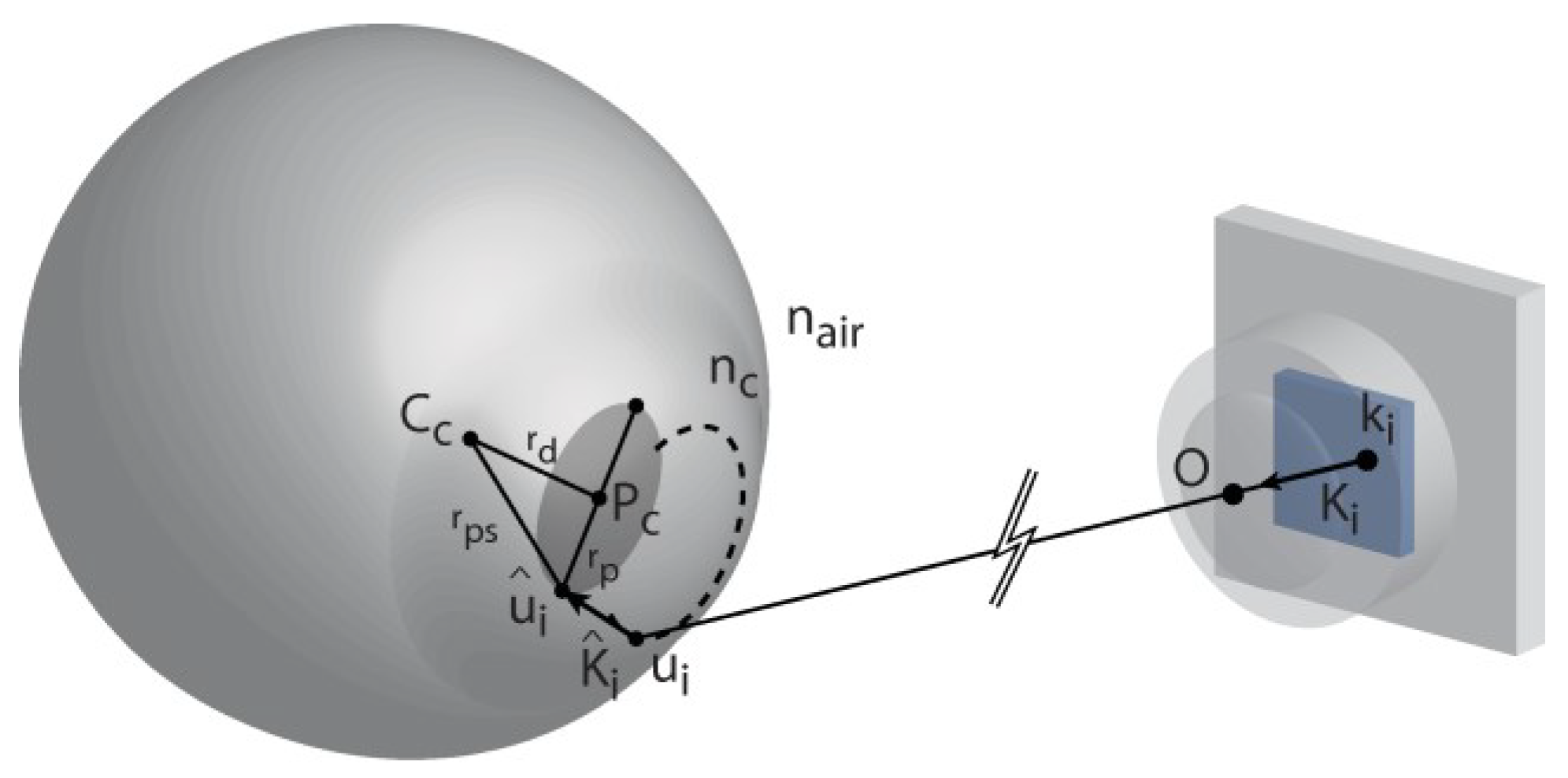
4.1. Cornea center computation

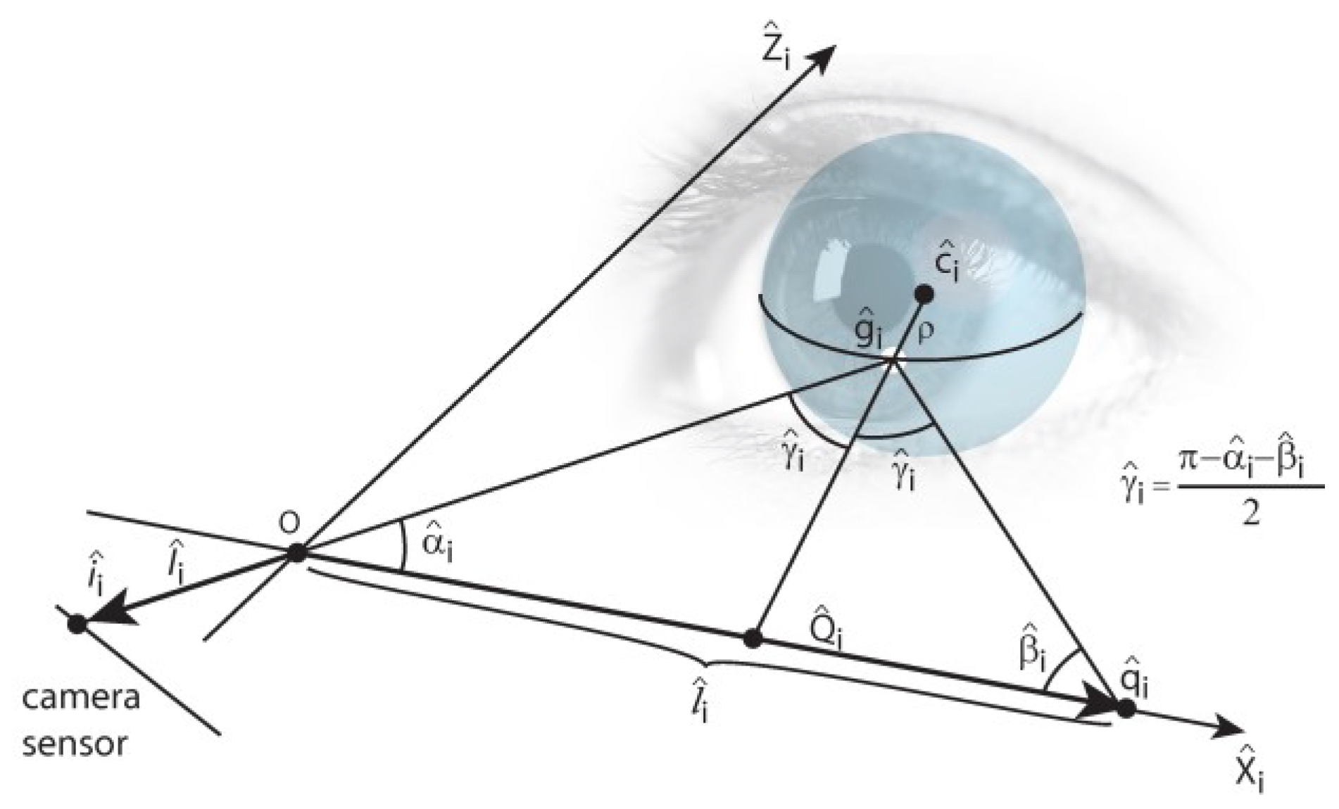
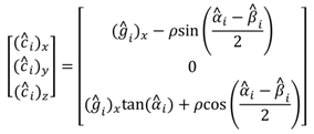
Computing the cornea center from the detected glints, Eq. (10), is done using a scheme that is presented by Hen-nessey et al. (2006) and Shih and Liu (2004) and explained here in brief. It is based on the law of reflection, according to which the LED source, its reflection from the corneal surface, the cornea center, camera’s optical center, and the image of the reflection on the camera’s image plane are all co-planar. Hence, we can form a glint specific auxiliary coordinate system whose origin is at the optical center of the camera, as described in Figure 4.

For the sake of clarity, the cornea center is denoted here with c. A light ray from q^ reflects at g^ and traverses through O and ^i i. Because the LED locations are assumed to be known in camera coordinates and the vectors ^I i (which point from O to ^i i) are known, it is possible to com-pute the rotation matrix R^i between the camera’s own co-ordinate system and the auxiliary coordinate system.

The cornea center can then be defined in the auxiliary coordinates as

(12)

where ρ is the (fixed) radius of the corneal sphere and

(13)

The cornea center in the auxiliary coordinates, ^ci, can be transformed back to the camera coordinates, c = R^−1 ^c, which results in an underdetermined system of 3 equations with 4 unknowns: (ci)x, (ci)y, (ci)z, and (gi)x. However, having at least two LED sources and corresponding glints provides an overdetermined system because the cornea centers equal (ci = cj∀j ≠ i) and so with two LEDs there are 6 equations and 5 unknowns. Each additional LED (and corresponding glint) increases the rank of the system so that the difference between the number of equations and unknowns behaves as 3NL − (3 + NL) = 2NL − 3 where NL is the number of LEDs. The resulting system of (non-linear) equations can be solved numerically using, e.g., Le-venberg-Marquardt method.

4.2. Pupil center computation

In the pupil center estimation, Eq. (11), we again fol-low Hennessey et al.(2006). The (3D) pupil center is com-puted as the average of different opposing points on the pupil perimeter. In order to determine the ith perimeter point, a ray is traced from its image point ki on the cam-era’s image plane, through the optical center O and point ui on the surface of the corneal sphere where the ray re-fracts according to Snell’s law towards the perimeter point u^i (see Figure 5).

Let us first estimate the point ui. The origin of the cam-era coordinate system is at the optical center so ui can be described with a parametric equation

(14)

because the point ui lies on the surface of the corneal sphere with center c and radius ρ, ∥ ui − c ∥= ρ, we have a set of 4 equations with 4 unknowns (si and the three com-ponents of ui) from which we can explicitly solve s and thus obtain ui.

Tracing the refracted vector K^ (with the known refrac-tive index of the cornea nc) gives another parametric equa-tion:

(15)

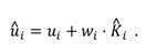
Because the distance between the pupil perimeter point and cornea center is ∥ u^i − c ∥= √r² + r² where r is given by population averages and rp is half of the length of the major axis of the fitted ellipse, we get a determined system of 4 equations with 4 unknowns (wi and the three components of u^i) which is solvable for wi. The perimeter point u^i can therefore be computed and the pupil center Pc can be estimated as the average of opposing points. We use two pairs of points: the endpoints of the major and minor axis of the fitted ellipse.

5. Locating the pupil features

The pupil detection is relatively straightforward, utiliz-ing conventional computer vision methods. Since the com-putation of the 3D pupil center requires locating at least two opposing points on the pupil perimeter, we search for an ellipse that most closely follows the pupil perimeter and use the endpoints of the ellipse axes for computing the 3D pupil center.

The opened eye image is cropped around the approxi-mate pupil center (see Section 2.2) and low-pass filtered. The filtered image is morphologically closed to emphasize the pupil using a circular structural element with size close to the pupil size. As this may, however, disturb the pupil edges, it is heuristically summed with the non-closed im-age. In order to achieve invariance to average brightness of the image, the summation image is scaled so that the intensity values are in the range [0,1]. The scaled image is thresholded, using a fixed threshold value. The connected components (“blobs") of the resulting binary image are computed, using a four-way connectivity. The blob that encloses the approximate pupil center is considered to be the pupil blob. The contours of the pupil blob are found and an ellipse is fitted to the found contours by minimizing the average distance between the ellipse and contour points (Fitzgibbon and Fisher 1995). Figure 6 gives an example of the filtered image, the binarized image, the found pupil contours, and the fitted ellipse.

Finally, in order to increase robustness against image noise, the endpoints of the major and minor axes of the fitted ellipse are filtered using the eye stability parameter θ (Eq. (1)) so that during the eye movements we would rely more on the measurements:

(16)

where u depicts any of the four endpoints and u^ is the cor-responding measured endpoint. The thresholding of θ with γmin is there to force the measurements to be always con-sidered by at least small amount. This is especially im-portant in case of smooth pursuits, during which θ can be too low.

6. Locating the cornea features

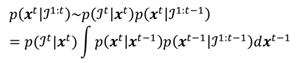
Locating the group of glints in the eye image is gener-ally a more complex task than locating the pupil. While the glints are typically very bright in the image, it should be easy to find the possible glint pixels by their intensity val-ues. However, the surface of the eye is approximately spherical and smooth only on top of the corneal bulge. On top of the sclera (the white of the eye), the surface is une-ven and can create additional distracting and distorted re-flections. Identifying true glints from the corneal surface is alleviated by the fact that the grid shape is relatively sim-ilar across eye images: the glints should approximately conform to a specific shape. In addition, during fixations the glints should appear at the same location as in the pre-vious video frame. These three assumptions about (i) the appearance of a glint, (ii) the shape of the glint grid, and (iii) the dynamical behavior of the glints can be combined within the Bayesian framework used here. The Bayesian approach allows locating the glint grid even when some glints may be occluded or distorted due to extra reflections or the eyelid. In our previous implementation (Lukander et al. 2013), the glints were identified heuristically; with the presented model grid based approach this error-prone step is avoided as an additional benefit.

6.1. Bayesian model for glints

Let x denote the glint grid, i.e., the coordinates of the glints in the eye image. The size of x is hence the number of LEDs, NL. The unnormalized posterior distribution for x, under Markov assumption, is

(17)

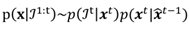
where $ℐ$^t denotes a “general" eye image, captured at time t. Due to our chosen likelihood function, we are unable to compute the integral in Eq. (17) in closed form since the (unnormalized) posterior distribution is not of a standard integrable function. The integral could be estimated with numerical methods, such as variational Bayes or Monte Carlo sampling. These methods are computationally heavy, making them unfeasible for realtime use. We thus use MAP (maximum a posteriori) estimate, that is, take the posterior to be a delta function at its maximum value:

(18)

where x̂^t-1 is the MAP estimate of the posterior at previous time instance. Thus the only data we have to store in memory is the previous estimate, x̂^t-1, and we can write

(19)

6.2. Implementation of the model

Section 2.2 presented cropping and opening of the in-put eye image and a method for finding the approximate pupil center in it. In a practical implementation of our probabilistic model for finding glints, the cropped image is filtered with the morphological top-hat operation, de-fined as the difference between original and opened image. The top-hatted image is cropped according to the pupil center and filtered using a small kernel to remove noise. This operated image is the input observation in the Bayes-ian model, denoted $ℐ$. An example of $ℐ$ is given in Figure 7.

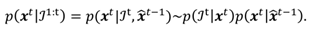
In our practical algorithm for finding the MAP esti-mate, the components are estimated one at a time. We are therefore interested on a conditional distribution, given the already estimated subset of the glint grid. The conditional posterior distribution for any component i of x^t can be written as

(20)

where x^t denotes the already estimated components of the parameter vector of which the likelihood is independ-ent. For convenience, we have dropped the “hat" symbol in the estimate of previous t so that x^t−1 ≡ x̂^t−1. Luckily, we do not need to know the normalization constant of the posterior as we are interested only on the relative values of it. Note that the dimension of a single glint xi is two as there are horizontal and vertical components. When esti-mating the first component, i = 1, there are no already es-timated components: x1:i-1 = x1:0 = {}, and x₁ must be esti-mated by other means (our way of doing this is described in Section 6.5).

6.3. Likelihood model

The likelihood function should give high values for the glint locations. As these pixels are assumed to be bright (see Figure 2B), a natural form for the likelihood is

(21)

where $ℐ$s is an eye image which is scaled by its maxi-mum value: $ℐ$s(x) ∈ [0,1] ∀ x, and β is a pre-fixed param-eter.

6.4. Prior model

Our prior assumptions are that, a priori to seeing a new image, the shape of the glint grid will be similar to what it is on average (in reality, the shape of the glint grid varies according to the position and rotation of the eye, and the individual shape of the corneal surface) and that the move-ment of the glints from the previous frame is in accordance with the estimated eye stability, θ. These assumptions are realized by combining two independent prior distributions, both modeled as Gaussian distributions.

The prior model for the shape utilizes a model grid which depicts how the glint grid is typically distributed, how it (co)varies, and its scale. For computing the model grid, a set of training images is collected and the glint lo-cations are manually annotated in each image. The average grid and covariance is computed from the collected point set in a mean and scale free space which makes the system invariant to the location and scale of the eye with respect to the eye camera(s). Including rotation invariance would be useless as the pose of the glasses with respect to user’s eyes is in practice always horizontal and the rotation invar-iance would only increase search space and computation time. An example of a model grid is shown in Figure 7. Note that the manual annotation needs to be done only once for each device setup (not for each user).

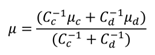
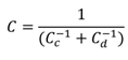
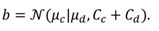
The grid point set is denoted with G and its covariance with CG. The “total" prior distribution is a product of the two Gaussian distributions:

(22)

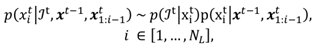
The subscript c stands for “conditional" and d for “dy-namical". The expected location of ith component of the conditional Gaussian, without yet taking the covariance into account, is

(23)

where E[⋅] denotes the averaging operation and s is the estimated scale. That is, to get the expected location of the current point (without covariance’s effect), the scaled dis-tance of the current point of the model grid to the average of previous points of the model grid is added to the average of previously estimated grid.

The scale s is estimated (when i > 2) as

(24)

where σu denotes the standard deviation of the hori-zontal components of the points and σv that of vertical components (note that xi is two-dimensional with horizon-tal and vertical coordinates). Thus, if the glints appear in the eye image in same scale as in the model grid, we have s ≈ 1; if the eye is closer to the camera or the corneal ra-dius is larger, compared to what was used for generating the model, we have s > 1. As more components are esti-mated (that is, i increases), the uncertainty in the scale es-timation decreases. For the second component (i = 2), the scale is the grid model’s scale, i.e., we assume the scale to be the average scale of the training samples used for build-ing the model grid (yet updated, see Subsection 6.6).

In order to compute the conditional mean and covari-ance, considering also the covariance CG , we partition x, G, and CG:

(25)

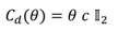
We get for the (scaled) conditional mean and covari-ance of the conditional prior distribution $𝒩$c :

(26)

(27)

where the term κ i 𝕀₂ regularizes the covariance (𝕀₂ is a 2 × 2 sized identity matrix). This is because as i gets larger, the covariance gets smaller and we found in prac-tice that eventually the prior distribution may restrict the search space too much. An alternative would be to use a prior distribution with heavier tails, such as the t-distribu-tion.

Let us study the “dynamical" prior distribution, $𝒩$d , of Eq. (22). Its mean value is simply the location of the cor-responding glint in previous image:

(28)

and the covariance is a diagonal matrix

(29)

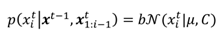
where c sets the upper bound for the diagonal elements. Hence, if the eyes seem to be in the same location as in the previous image based on the eye stability estimate de-scribed in Section (2.3), the glints are searched for in the close vicinity of their corresponding previous location and if the eye seems to be moving, the search space is in-creased. Note that θ ∈]0,1[ and due to the ubiquitous and omnipresent image noise, θ is always clearly positive. However, one might want to use a lower bound on the di-agonal elements of (29) to be on a safe side with its inver-sion.

Finally, the combined prior distribution, which is the product of two Gaussian distributions (22), is another Gaussian:

(30)

where

(31)

and

(32)

and the normalization factor is

(33)

6.5. MAP estimation

As mentioned in Section 6.1, for the glint locations, we search for values that maximize the posterior distribution: the MAP estimate. This is done by maximizing Eq. (20) one component at a time. In order to increase robustness, instead of a single MAP estimate many estimates are searched independently by using different ordering for the components of x^t. As this approach resembles Particle fil-tering – also known as Sequential Monte Carlo sampling (Doucet, De Freitas, and Gordon 2001) – we call the inde-pendent searches “particles" which may be considered as hypotheses for the parameter values. For examples on us-ing Particle filtering for locating image features, see (Tam-minen and Lampinen 2006; Toivanen and Lampinen 2011).

First components of the particles are initialized in the brightest pixel locations of the image $ℐ$. The number of these “candidate" glint locations is denoted Ngl.cand.. For each such candidate location, NL particles are initialized with different component order. Hence, the number of par-ticles is Npart. = NL × Ngl.cand..

When searching the Ngl.cand. brightest image pixels, the vicinity of the previously found location is overpainted so that neighboring pixels will not be chosen. The glint can-didates may naturally contain also false glints but the more candidate points there are, the higher is the probability of correct glints being chosen. After each particle has searched their MAP estimates, they are compared and the one with the largest maximum value of the joint posterior (i.e., product of the MAP values of the conditional distri-butions) is defined as the “winner" whose parameter val-ues are taken to be the final MAP estimate. Figure 8 exem-plifies the MAP estimation procedure.

Note that the used method always localizes the glints, whether they are visible or not. Non-visible glints are lo-cated in their supposed location as suggested by the grid model (that is, prior). Figure 9 illustrates such a case. How-ever, when computing the cornea center (see Section 4.1), including the estimated location of the non-visible glints may increase the estimation error as opposed to including only the visible glints. Therefore, the cornea center is com-puted from a subset of the detected glint grid which con-sists of glints whose score exceeds a threshold. The score is defined simply as the intensity value at the glint in the scaled image, i.e., log likelihood (Eq. (21)) divided by β. The allowed minimum size for the subset is naturally two to be able to solve the 3D cornea center. Figure 10 gives an example of having additional distracting reflections around the “correct" glint. With a reasonable prior model, the MAP estimate is at the correct location.

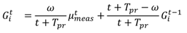
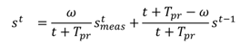
6.6. Updating glint grid

The shape of the glint grid, G, varies from person to person, mainly due to different eye shapes. As noted, we use an average glint grid model which is a typical repre-sentation of the grid. This grid model can be modified to adapt to the personal grid by updating the mean, covari-ance, and scale recursively:

(34)

(35)

(36)

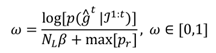
where Tpr is the number of prior measurements assumed to have occured before the first frame and where the weight ω is defined as the logarithm of the MAP value di-vided by the largest possible value for the logarithm of the posterior:

(37)

where max[pr] is the sum of the maximum values of the logarithms of the conditional prior distributions, Eq. (30), summed over the components.

7. Kalman filter

Despite all the advanced tracking algorithms for the glints and pupil, the estimated gaze point is often still noisy. This is understandable since even the tiniest differ-ences in the glint locations or the endpoints of the fitted pupil ellipse cause deviation in the calculated gaze point. Because images always contain noise, the estimations of the eye features, and therefore also the gaze point, fluctu-ate even when steadily fixating a single point. This is at best just irritating but often disturbs the analysis and can even make the use of gaze information impractical.

As a remedy, the gaze point is smoothed by Kalman filtering which has been shown to improve performance (Toivanen 2016). A Kalman filter produces a statistically optimal closed form point estimate for the unknown state of a linear dynamic model which has Gaussian distribu-tions for process and observation noises; see, e.g., Särkkä (2013). A Kalman filter can predict the state also in case of missing observations which may happen here if the eye features of both eyes are misdetected. Comparing to prior work, Zhu and Ji (2005) used a Kalman filtering for track-ing the pupil and Komogortsev and Khan (2007) used Kal-man filter directly on the gaze signal, as is done here, but they had no observation model for the velocity component which compromises the performance with a noisy signal.

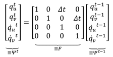
Let us denote the horizontal and vertical gaze coordi-nates (in the scene camera) at time instance t with q^t and velocity observations could q^t and their velocities with q̇ and q̇ . The movement of the gaze point is assumed to be piece-wise linear so that the state can be modeled to evolve linearly as

(38)

The process is assumed to be noisy with zero-mean Gaussian distribution so we get

(39)

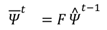
where Q^t is the covariance of the process noise. The pre-dictions for the state estimate (Ψ ) and its covariance (P ) at time instance t, given the previous estimates Ψ^ t−1 and P^t−1, are

(40)

(41)

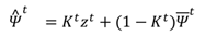
Gaze coordinates and their velocities are measured with a zero-mean Gaussian noise distribution. The obser-vations z^t at time t are thus related to the state by

(42)

where R^t is the covariance of the measurement noise. The (unknown) true state Ψ^t of the system, depicted with Equations (39) and (42), and its covariance P^t can be esti-mated as

(43)

(44)

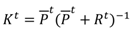
that is, the estimate for the state is a weighted average of the latest measurement and the prediction. Computing the weight as

(45)

is known as Kalman filtering.

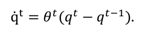
The gaze point observations are naturally the estimated gaze points, see Eq. (7). The velocity observations could be simply the derivative of the gaze point observations but then the noise in the gaze point estimates would affect the velocity estimates, too. A better approach is to utilize the eye stability parameter θ since it is (almost) independent on the gaze point estimates. This is beneficial especially during fixations when the pixel-wise difference in subse-quent eye image frames is close to zero (⇒ θ ≈ 0) while the difference in gaze point estimates can be relatively large. Because θ only estimates the amount of movement, the direction of the velocity is computed from the gaze point estimates and the velocity observations are

(46)

One problem with the presented Kalman filter is that the saccades are relatively sudden and fast which can lead to the assumption about the piece-wise linearity failing, es-pecially with a low frame rate (like 30 fps). Luckily, the covariances of the process noise (Q^t) and measurement noise (R^t) can depend on the time instance t, that is, they can be modified realtime. Here the process covariance is taken to be constant, Q^t ≡ Q ∀t, but the measurement co-variance is modified in realtime so that the larger the ve-locity estimate, the more the location observations are trusted and when the eyes seem to fixate, the location pre-dictions are trusted more. In practice, this means that the gaze signal is filtered (almost) only during fixations; dur-ing saccades and blinks, the Kalman filtered gaze point ap-proximately equals the “raw" gaze signal. The covariance of the measurement noise is defined as a diagonal matrix

(47)

where Rv is a constant variance of the velocity observation and R^t is a time-dependent variance of the location obser-vation:

(48)

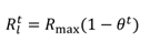
where Rmax is a pre-fixed maximum variance for the meas-urement noise. Remember that θ ≈ 1 during and also slightly after the saccade so there is a small lag after be-ginning of a fixation before the signal is filtered heavier, exactly as wanted. Due to the modification of the measure-ment noise, the Kalman filtering causes no latency.

If the measured point is clearly outside the image area or if the measured velocity exceeds a threshold (as often happens during blinks), the measurement is considered an outlier; in this case, the prediction is used for the estimated location and the velocity is set to zero.

8. Algorithmic nutshell

The whole algorithm of tracking the gaze point is re-capped below. The number in brackets shows the corre-sponding sections and subsections.

• Preprocess eye images (2.2)

  (a)

  Transform the images into grayscale and open and crop the images

  (b)

  Locate the approximate pupil centers

• Estimate the eye stability (2.3)

  (a)

  Localize glints (6)

  (b)

  Use the likelihood and prior models (6.3, 6.4)

  (c)

  Estimate MAP (6.5)

• Update the model glint grid (6.6)
• Localize pupil (5)
• Estimate cornea center (4.1)
• Estimate pupil center (4.2)
• Perform user calibration, if not already done (3.2)
• Compute POG (3.3)
• Kalman filter (7)

Sometimes the localization of pupil and/or glints fail (steps 3 and 4 above). In case of pupil, the failure can be deduced from the difference between the left and right pu-pil sizes which should approximately match. The validity of the estimated glint locations is inferred from the weights ω, see Eq. (37). Thresholding the weight, either of the gaze vectors can be excluded from the computation in which case the gaze point in Section 3.3 is computed using the “good" eye only and the gaze distance is estimated to be the previous successfully estimated distance. If features from both eyes are poorly localized, the frame is concluded to be part of a blink, during which the eyelid naturally oc-cludes the pupil and glints.

9. Experimental evaluation

This section evaluates the performance of the presented algorithms. First, we present our hardware and software solutions, used for testing the algorithms. Next, we intro-duce the experimental setup, provide the used parameter values, and show some qualitative results. Then we present the performance measures which are used for reporting the numerical performance. Finally, we discuss the challenges of the system through some example cases. The study pro-tocol has been reviewed by the Coordinating ethics com-mittee of the Hospital District of Helsinki and Uusimaa. The recorded data is published openly (https://github.com/bwrc/ooga/tree/master/public_data).

9.1. Hardware and software

For testing and utilizing the presented algorithms we have built a glasses-like 3D printed headgear where the cameras and circuit boards are attached (see Figure 11). The cameras are standard USB cameras that have no IR filters and have high pass filters inserted for blocking vis-ible light. For both eyes there is a circuit board powering six IR LEDs, powered via the USB camera cables. As the frame is 3D printed, the positions for the cameras and LEDs relative to the cameras are extracted from the 3D model. The cameras we used capture images with VGA (640 x 480 px) resolution. The average frame rate during the experiments was 25 fps (the cameras used have a fixed iris, and the frame rate depends on available illumination). The safety issues were considered in the design so that the overall emitted radiation power is in line with the safety standard IEC 62471 (International Electrotechnical Com-mission 2006).

Figure 11. The implemented gaze tracking glasses. There are six LEDs around each eye. The scene camera is lo-cated above the nose.

Figure 11. The implemented gaze tracking glasses. There are six LEDs around each eye. The scene camera is lo-cated above the nose.

We have implemented all the presented algorithms in C++ utilizing the following libraries: The OpenCV library for computer vision tasks, the Eigen library for matrix op-erations, the GSL library for numerically solving the sys-tem of nonlinear equations in estimating the cornea center, and the Boost library. During the experiments, for maxi-mum control, the software was used just to record the vid-eos which were processed afterwards with a Dell E6430 laptop (containing i5-3320M @2.60 GHz and a Linux Ub-untu 16 LTS operating system).

9.2. Experimental setup

The performance of the presented system, and for ref-erence the commercial SMI system (with iView 2.1 re-cording software and BeGaze 3.5 analyzing software) was tested in a laboratory setting with 19 participants (9 males, age 31 ± 8, all had normal vision with no corrective op-tics). The subjects sat in a chair in a dimly lit room (the lighting in the room was dim to enable automatic detection of the gaze targets in the scene video) and viewed a display while wearing the gaze tracking glasses whose camera streams were recorded. Different gaze distances were used to test performance outside the calibrated distance. The ex-periment included three different displays with three view-ing distances (a 24” monitor at 60 cm, a 46” HDTV at 1.2 m, and a projector screen at 3.0 m) so that at each distance the resolution of the stimulus was adequate and the viewed stimuli spanned a similar visual angle.

The subjects were asked to sit relaxed and hold their head still during the measurements. User calibration was performed at only one of the three viewing distances for each subject. The presentation order of the displays and the calibration distance was permuted between the participants and each calibration distance was used equally often.

The calibration procedure cycled a stimulus dot through nine different locations on the selected calibration distance. The duration of the fixation stimuli was jittered between 2–3 s to prevent anticipatory gaze shifts. To de-crease artifacts in the evaluation data, after every third lo-cation the dot changed from black to gray for three seconds signaling the subject to blink freely, while avoiding blinks during the rest of the sequence. The actual calibration of the system in this scenario was performed offline as de-scribed in Section 3.2.

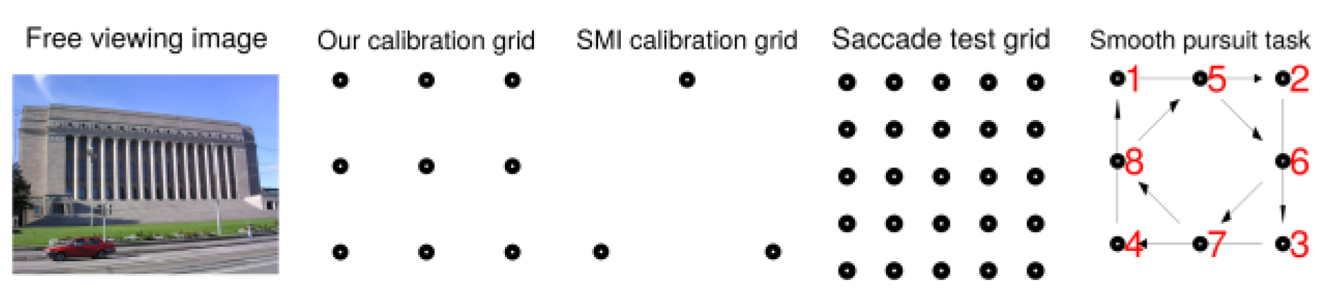
The calibration also included a 20-second free viewing task with a picture of the Finnish Parliament House (the leftmost image in Figure 12). The stimulus was selected to supply evenly spread fixation targets across the image sur-face. The data recorded during free viewing was used for forming the initial grid model by manually annotating glint locations in ten eye images (per eye) for each subject. In the evaluation, a grid model was constructed from all the other subjects’ glint location data but the one being meas-ured, as a leave-one-out scenario, to avoid overfitting. The SMI offers a 1-point and 3-point calibration routines; we used the 3-point calibration, with a triangle of dots (see Figure 12).

The test phase comprised two tasks: a saccade task and a smooth pursuit task. The saccade task included 25 stim-ulus locations forming a regular 5 × 5 grid – see Figure 12 – with a random presentation order (however, matching between subjects). Again, blinking was discouraged ex-cept after every third stimulus location ending with a blink pause. The smooth pursuit task presented a dot moving with a constant velocity of 3.0 degrees per second. The se-quence is depicted in the rightmost panel of Figure 12. In each corner, the dot stopped for the blink pause. In each phase and for each distance, the size of the dot was one degree and the dot grid spanned an area of 24 degrees in both directions.

The performance of the presented and the SMI system was evaluated by running each stage two times, once for each system. For both devices, the calibration was per-formed at the first presentation distance and the same cal-ibration information was used for all distances. The track-ers were swapped during each distance and between changing distances and the order of the glasses was bal-anced, each system going first the same number of times.

Unfortunately, some human errors were committed during the recordings. For two subjects, the recordings for the calibration phase were accidentally deleted. In these cases, the first nine fixations in one of the other two sur-viving test phase recordings were used for user calibration. Additionally, for one subject the calibration display was not fully visible in the scene camera recording, inhibiting performing the calibration. One subject wore heavy mas-cara, challenging pupil detection for both systems, and the SMI calibration for one subject was poor. These anomalies are reported in

Table 1. The anomalies of the dataset.

.

The videos, recorded during the experiments, were pro-cessed using the presented method, producing gaze coor-dinates in scene camera coordinate system, the weights ω (see Eq. (37)), blink classification, and estimated gaze dis-tances. If the frame was classified as a blink, it was not used in the analysis – sometimes the participants blinked also when not supposed to. The videos were also processed with the SMI software, outputting the gaze coordinates and event classification (a fixation, blink, or saccade).

9.3. Parameter values

The algorithms require a set of fixed parameters, tuning their performance. However, the system is not very sensi-tive to these as long as they are within a “reasonable" range. The parameters, their explanations and the values used are tabulated in Table 2. These values were found to give satisfactory performance during previous testing, i.e., they were not optimized in any sense for this particular da-taset. The physical eye parameters were as follows: cornea radius ρ = 7.7 mm, the refractive index of cornea nc = 1.336, and the distance between cornea center and pupil plane rd = 3.75 mm.

The most effective parameters are probably the likeli-hood steepness β, the prior covariance regulator κ, and the threshold parameter in the pupil detection. Computation-ally, the most demanding part is the MAP estimation of the glint locations. There, the computation time is directly pro-portional to the number of particles, i.e., the number of glint candidates (Ngl.cand.) multiplied by the number of LEDs. Therefore, we also investigate the effect of decreas-ing Ngl.cand. on performance and computation time.

Table 2. The parameters of the model, their explanation, the corresponding equation or section in the text, and the values used.

param.	explanation	in text	value
β	likelihood steepness	Eq.(21)	100
κ	prior covariance reg-ulator	Eq.(27)	1
c	max. variance in dyn. prior	Eq.(29)	100
Q	process variance in Kalman filter	Eq. (39)	1
Rv	velocity meas. vari-ance in Kalman filter	Eq. (47)	1
Rmax	max. meas. variance in Kalman filter	Eq. (48)	100
λm	sigmoid parameter	Eq. (2)	0.02
αm	sigmoid parameter	Eq. (2)	500
w	increase of θ after saccades	Eq. (1)	0.7
Tpr	number of prior measurements	Eq. (36)	10
γmin	minimum θ value in pupil detection	Eq. (16)	0.2
Ngl.cand.	number of glint can-didates	Sec. 6.5	6
thold	threshold in pupil de-tection	Sec. 5	0.2

Table 2. The parameters of the model, their explanation, the corresponding equation or section in the text, and the values used.

param.	explanation	in text	value
β	likelihood steepness	Eq.(21)	100
κ	prior covariance reg-ulator	Eq.(27)	1
c	max. variance in dyn. prior	Eq.(29)	100
Q	process variance in Kalman filter	Eq. (39)	1
Rv	velocity meas. vari-ance in Kalman filter	Eq. (47)	1
Rmax	max. meas. variance in Kalman filter	Eq. (48)	100
λm	sigmoid parameter	Eq. (2)	0.02
αm	sigmoid parameter	Eq. (2)	500
w	increase of θ after saccades	Eq. (1)	0.7
Tpr	number of prior measurements	Eq. (36)	10
γmin	minimum θ value in pupil detection	Eq. (16)	0.2
Ngl.cand.	number of glint can-didates	Sec. 6.5	6
thold	threshold in pupil de-tection	Sec. 5	0.2

9.1. Qualitative performance

Figure 13 exemplifies a gaze tracking signal, blink events, and sigmoid values of Eq. (2), estimated from a video material recorded during the saccade and smooth pursuit tasks. The signal seems to behave smoothly during fixations, as expected from the utilized Bayesian tracking algorithms and Kalman filtering. On the other hand, the signal succeeds to follow the saccadic behavior without an “overshooting" effect, owing to the modified measurement variance of the Kalman filter. Also the sigmoid value, which reveals the stability of the eye images, seems to be-have as assumed: close to zero during fixations and unity during saccades. The signal seems reasonable during the smooth pursuits, too, albeit the signal “jerks" a bit when the stability is estimated to change. Remember that during blinks, the POG estimate is typically the Kalman filter pre-diction.

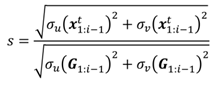
9.5. Performance measures

For an automatic performance analysis, the scene cam-era videos were processed with a Matlab script which au-tomatically localizes the stimulus dot, allowing the com-putation of the error between the estimated and true values and thereby the numerical performance. For analyzing gaze location accuracy, after each stimulus movement a period of one second was excluded from the analysis; it was assumed that the corresponding reaction time and sac-cade time was never longer than one second.

As performance measures, we report accuracy and pre-cision. Accuracy is defined as the angular error between the estimated gaze point and target point (Holmqvist et al. 2011). Note that the “true" fixation target remains un-known – we can only hope that the subjects were really fixating the dot. The angle is estimated by using the known gaze distance, the metric distance between the gaze and target points, and a right triangle rule. For computing the metric distance between the points, the mm per pixel rela-tion was estimated using known real-world dimensions of the displays and annotating the corresponding points in a few representative video frames

Precision reflects the ability of the eye tracker to relia-bly reproduce the same gaze point measurement and is thus related to the system noise. Good precision is desired in, at least, gaze based interaction and fixation analysis as noisy estimates during single fixation may be misclassified into several short fixations. Precision is usually defined as a root-mean-square (RMS) or root-median-square (RMedS) value of subsequent angular errors between esti-mated and target points, q^est and q^target, measured during a fixation (or a separate smooth pursuit movement) (Holmqvist et al. 2011). The RMS value would thus be

(49)

where Nf is the number of fixation samples and D is the gaze distance (note that q’s are metric vectors here). RMedS would be similar but using a median value of {ϵ², i = 1, . . . , Nf − 1} instead of mean. In addition, we re-port the standard deviation of the angular errors during a fixation (or smooth pursuit) as an alternative precision measure.

9.1. Numerical performance

The accuracy values of each subject in saccade and smooth pursuit tasks are given in Figure 14 for both gaze trackers. The figure shows the 25th, 50th (median), and 75th percentile values of the accuracies for all three gaze distances concatenated.

. Our tracker seems to outperform the SMI system with most of the subjects. In addition, the performance of the presented system stays relatively equal for each subject, whereas SMI’s varies a lot. The SMI’s accuracies of ID13 are out of figure range, with its median values being 19 and 17 degrees for saccade and smooth pursuit tasks. In our gaze tracker, subject ID06 performs poorly due to mascara.

Evaluating a “winner" from the median values and per-forming a pairwise Fisher Sign Test gives a p-value of only 0.0044 for the null hypothesis that ours and SMI systems perform equally well. We can therefore conclude that in this task our system outperforms the SMI’s (P=0.0044, pairwise two-tailed Fisher Sign Test).

A possible explanation for the difference in the perfor-mances is SMI’s apparent intolerance to the movement of the frame; based on our experiments, even slight change in locations of the cameras and LEDs with respect to the eye caused deviation in SMI’s estimated gaze point. Hence, the SMI glasses should not be moved at all once calibrated. In the experimental setup, however, the glasses were switched during each gaze distance and between them so the glasses were taken off and put back on after each dis-tance change. The presented system is invariant to the movement of the glasses – as long as the eye camera sees the pupil and at least two LED reflections, the fixated gaze point is stationary. 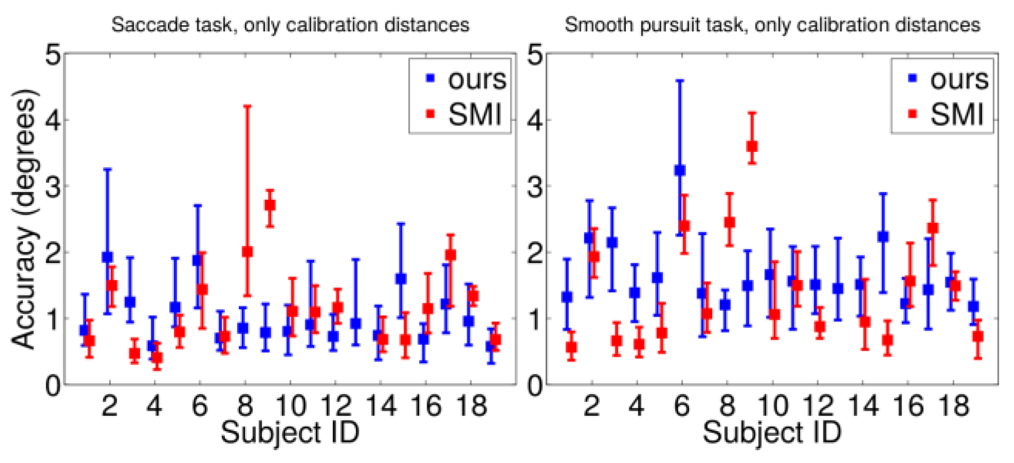Figure 15 illustrates the errors only for the calibration distances, including thus only the record-ings of the test phase following the calibration phase. Here the accuracy values for the SMI system show clear im-provement.

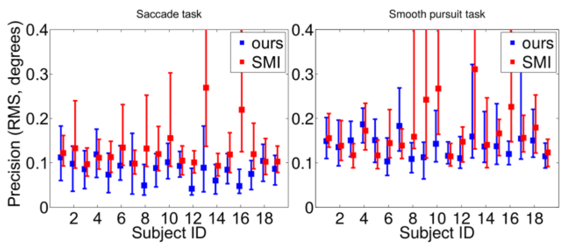
The precision (RMS) values are presented in Figure 16. For each subject, the RMS values of the subsequent angu-lar errors between estimated and actual target points for each fixation are concatenated over the three gaze dis-tances and the percentile values are computed from these. On average, the presented system provides better precision than the SMI device and the behavior is more or less sim-ilar over the subjects. For both systems, the precision is worse in the smooth pursuit task. In our case, this is be-cause the tracking components, especially the pupil ellipse end points tracker and Kalman filtering, may lag if the eye is estimated to be stable, as is the case during a smooth pursuit.

The averaged results of all subjects are tabulated in

Table 3. The performance over all test subjects’ data for both the saccade and smooth pursuit tasks, for the presented device (“ours") and the SMI system, in degrees of visual angle. The leftmost column lists the device; next four columns report the mean, median, ω-weighted mean (see Eq. (37)), and standard deviation (STD) values of accuracy; three rightmost columns report the precision measure which are the average root-mean-square (RMS) and root-median-square (RMedS) values of subsequent angular errors between estimated and target points during fixations or a smooth pursuit movement, and an average standard deviation of the angular errors during a fixation or a separate smooth pursuit movement (STD(a)). Before computing the values, the results from all gaze distances were concate-nated. The superscripts c refer to using data only from the calibration distance and * refer to excluded recordings ID06, ID07, ID11, and ID13 (see Table 1 for explanation). The values at the bottom show the average missing value rate in percentages, that is, the ratio of blinks and unavailable measurements to the number of all events. In each pair of ours and SMI results, the better result is written in italics. Lower values are better.

, which shows the outstanding numerical performance of the presented system – the mean and median accuracy of the saccade task is 1.68 and 1.20 and the RMS precision is 0.12 degrees of visual angle, averaged over all the sub-jects and viewing distances. Dropping the anomalous test subjects, as reported in Table 1, out of the analysis im-proves the performance and computing the results only for the distance where the device is calibrated gives even bet-ter results; half of the time the error is less than 0.92 de-grees. The probable reason for the slightly poorer perfor-mance when including also the data from other viewing distances is that the calibration scheme optimizes the cor-rection matrix R to give best accuracy in the calibration distance – remember that R is not a pure rotation matrix and it aims to correct all error sources there are, from im-perfect hardware calibration to incorrect eye parameters for the user. Still, the values of Table 3 demonstrate that the presented system performs well in all gaze distances. The performance in the saccade task is generally better than in the smooth pursuit task.

In the third column (“W. Mean"), the POG values have been weighted by the average of left and right eye’s weights ω which was defined as the logarithm of the MAP value of the fitted glint grid, divided by the largest possible value for the logarithm of the posterior (see Eq. (37)). This is another benefit of the probabilistic approach: we natu-rally get a “score" for the estimation, reflecting the (un)cer-tainty about it. For SMI, such value is unavailable and we used unity weights there so the weighted mean equals the ordinary mean. As our weighted mean values are better than ordinary means, the ω seems to indeed reflect the un-certainty about the gaze point estimate and taking it into account improves the results.

As mentioned, SMI clearly suffers from the movement of the frame after calibration, resulting in decreased accu-racy. However, the presented solution outperforms the SMI, in terms of accuracy and precision, also when includ-ing only the calibration measurements. The SMI performs better only in the smooth pursuit task at the calibrated dis-tance when the “bad" subjects’ data are removed. Our sys-tem also fails on less samples (SMI 17.4 % vs. 11.2 % in-cluding all data) and while these numbers include periods during blink breaks, there is no reason to suspect that the blinking behavior would differ between the devices so our system more often produces a valid measurement.

As a final comparison between the two systems, Figure 17 shows the histograms of accuracies in the saccade task, excluding the anomalous cases. Accuracy values for the presented systems are clearly concentrated around lower error values, whereas the distribution of the SMI device is wider, including values with larger errors.

Table 4. Real and estimated gaze distances (mean, me-dian, and STD), in meters, using all the data.

Real value	Mean estim.	Median estim.	STD of estim.
0.60	0.59	0.59	0.32
1.20	1.10	1.01	0.77
3.00	2.72	1.81	5.67

shows estimations of gaze distances with the presented system, including all the test data. The shorter distances seem to be more accurate than the largest dis-tance whose distribution is skewed due to some very large distance estimations, manifesting also as a large difference between the mean and median values. For 3D gaze points this might present a problem. However, when the gaze dis-tance is larger than three meters, the vergence angles of the eyes are practically in parallel and estimation errors above introduce very small changes to the 2D projected gaze point at these distances.

The effect of decreasing the number of glint candi-dates, Ngl.cand., and thereby the number of particles in the glint finding algorithm was studied by running the results again with value Ngl.cand. = 2 (corresponding to 2×6 par-ticles) instead of Ngl.cand. = 6 (36 particles). The compu-tation times were estimated by processing one of the rec-orded videos with the two different values for Ngl.cand.. The results are given in

Table 5. The result of comparing two different values for N_(gl.cand.), using all the data. The columns refer to mean and median accuracy, RMS precision, missing value rate, and mean and median computation times of single frame in milliseconds. The unit of accuracy and precision is degrees. Lower values are better.

and indicate that dropping the parameter value has a negligible effect on the perfor-mance but a large effect on the computation time. The lower particle number does have a slight effect on the rate of missing values as the algorithm may fail to find a good fit for the glint grid in difficult cases where only a small number of the glints are visible. Even with 36 particles, the running time of the algorithm is below 33ms, enabling realtime handling of 30 fps camera streams, whereas using 12 particles allows to process 80 frames per second.

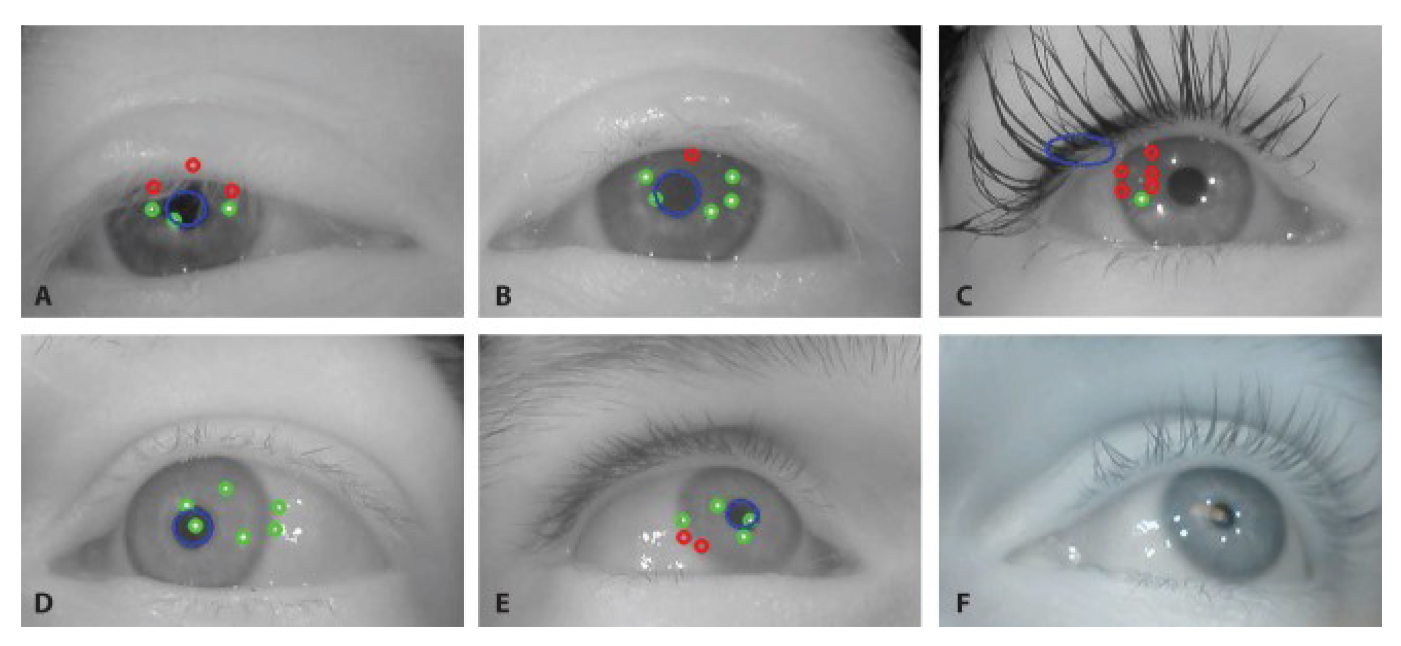
10. Challenges

While the presented solution seems robust for all eyes encountered so far, the dynamic, variable nature of eye im-ages presents occasional challenges for the algorithms. Typical examples of performance with artefactual images are presented in Figure 18: Half-closed eyelids or eyelids occluding the pupil and part of the glints as well as miss-ing, extra, or distorted reflections from the surface of the sclera outside the corneal bulge are generally well handled. The failure of approximating the initial pupil due to, for instance, heavy mascara ruins the performance. Addition-ally, external IR sources such as sunlight can create extra reflections and even block some of the features – the bot-tom right panel of Figure 18 exemplifies this.

11. Discussion and Conclusions

This paper has presented algorithms for tracking gaze with a mobile wearable device. The algorithms are based on a physical eye model, computer vision methods, Bayes-ian tracking of glints and a particle filter like method for computing the MAP estimate, binocular gaze estimation, and Kalman filtering. The main mathematical contribu-tions are in locating the LED reflection (glints) and the pu-pil in the 2D eye image robustly, performing user calibra-tion, and Kalman filtering the estimated gaze point in the 2D scene camera coordinates. The promise of the method was evaluated in experiments where 19 test subjects viewed a moving dot on three displays with different view-ing distances. Publication of this experimental data is an-other of our contributions. Benefits of an open source pub-lication compared to a proprietary architecture are that the full system becomes documented and the system can be modified for different needs; one can easily adjust any part of our algorithm, from image processing to system output. An additional contribution is testing the commercial SMI Eye Tracking Glasses – to the best of our knowledge, this is the first study to make a proper “scientific" quantitative evaluation of its performance.

The results show that when fixating only on the cali-brated distance, our spatial accuracy is approximately one degree of visual angle; the median is slightly below, and ordinary and weighted means are slightly above one de-gree. When viewing also other distances – as is the case in natural viewing conditions – the accuracy deteriorates slightly. This is because the user calibration not only cor-rects the deviance between the measured optical vector and the “real" gaze vector, but also compensates for the other imperfections of the eye model and algorithms, and is op-timal for the calibrated distance. However, the perfor-mance is good also when averaged over all the viewing distances: the median is 1.17 and weighted mean is 1.55 degrees when excluding the “anomalous" subjects. Addi-tionally, it should be noted that the automatic localization of the target point in the calibration procedure is imperfect and the corresponding error is included in the computed error – the real error in accuracy is thus likely less than the reported values (this of course applies to SMI, too). It can be concluded that during fixations, our accuracy is better than 1.5 degrees. The precision is also fairly good: the av-erage root-mean-square and root-median-square values of subsequent angular errors between estimated and target points during fixations are approximately 0.1 degrees. Also in the smooth pursuit task, with a moving target, the accuracy is better than two degrees.

The performance of the commercial SMI system is, in general, worse – the mean accuracy over all subjects is four degrees. This is mostly due to the intolerance of the SMI system against the movement of the device; due to the ex-perimental setup, the device had to be removed after re-cording the calibrated distance. Including only the cali-brated measurements gives better results but our system outperforms here, too, both in terms of accuracy and pre-cision. Additionally, our system has a lower missing value rate. The intolerance against device movement is problem-atic for the SMI device in practical measurements because it necessitates monitoring the subjects during the measure-ments and the experiment must be aborted when the device moves and the subject needs to be re-calibrated. Due to the model-based approach, our system provides tolerance against device movement. Another nice feature of our sys-tem owes to the probabilistic approach: the estimates can be weighted by their certainties, allowing more robust es-timation of the metrics that depend on the gaze point, such as the accuracy measure in our experimental evaluation.

During user calibration, the glints were sometimes misdetected and the corresponding gaze point could not be utilized in the calibration process. These were mostly some of the four corner points of the 3 × 3 dot grid which the subjects viewed in such a wide angle that the LEDs were reflected completely outside the corneal bulge. In retro-spect, in order to ensure the quality of the calibration sam-ples it would had been wiser to calibrate while recording, as is done in “live" usage – if the glints are not properly detected, the user is asked to move the head slightly until they are found. The user calibration scheme of SMI con-sisted of only three calibration points (three is the maxi-mum) and is therefore lighter to perform than our calibra-tion. While three points is theoretically enough for our cal-ibration, too, the used nine points which approximately cover the viewing area give a more reliable estimate of the calibration matrix.

Computationally, the biggest effort is spent on finding glints. The computation time here is controlled by the number of particles. The results show that, at least in this setup, the performance is similar between 36 and 12 parti-cles while the corresponding processing times were 30 and 12 ms per frame. However, in more challenging environ-ments with distracting reflections from external sources, e.g., sunlight, the particle number may have a larger effect on the performance. Using more particles gives more ro-bustness at the cost of computation time. In a practical im-plementation, the glint search process could be sped up by parallelizing each (independent) particle by making them run in their own threads or even utilizing hardware accel-eration. A ruder trick would be to skip the glint and pupil estimation if the eyes seem to be fixating (and the fixation has lasted for few frames) which can be assessed from the stability parameter θ. As most of the viewing time in typ-ical applications is spent fixating, this would speed up the computation significantly.

All algorithms and calibration routines were written in C++. Due to the involvement of the GSL library, the soft-ware is currently licensed under the GPL, version 3, while solutions for a more permissive license are sought for. The project is released in Github: https://github.com/bwrc/ooga. (OOGA is Open-source GAzetracker).