Downside-Sensitive Portfolio Optimization and Risk Overlays for Real Estate Securities

Abstract

We employ an empirical framework for real estate securities that incorporates portfolio optimization, return distribution tail diagnostics, risk metrics, modeling of long-range dependence in return volatility, regression against benchmark indices, and option pricing, treating these as necessary layers of a risk-management structure that concentrates on downside risk. Optimization compared mean–variance against downside-sensitive conditional value at risk. Tail behavior was assessed via skewness, kurtosis, and extreme value theory; volatility persistence was examined using ARMA–FIGARCH models. Benchmark dependence was examined via the capital asset pricing model (CAPM), employing endogenous and exogenous market proxies. Insurance instruments via European options were priced using a doubly subordinated normal inverse Gaussian pricing model capable of modeling skewed, heavy-tailed return distributions. Significant findings for the optimized portfolios include return distributions with losses that are heavier-tailed than gains; a transition in time from moderate-to-high long-range dependence in conditional volatility; smaller values of CAPM “alpha” and “beta” for minimum-risk portfolios compared to tangent portfolios; and significant implied volatility values.

1. Introduction

A Gaussian-based framework of portfolio optimization (e.g., mean–variance, Black–Litterman), risk measures (e.g., Sharpe ratios), and insurance instruments (e.g., Black–Scholes–Merton pricing), combined with non-parametric risk assessment (e.g., maximum drawdown), is a consistent model framework, but is well known to be “blind” to the stylized facts of asset returns and therefore vulnerable to market disruption. A mixed framework combining tail-aware optimization (e.g., CVaR) with Gaussian-based risk measures and insurance instruments incurs additional risk due to cross-model errors. We discuss the implementation of a framework consisting of portfolio optimization, return distribution tail analysis, risk metrics, and option pricing performed under a consistent emphasis on the stylized facts (skewness, kurtosis, heavy tails, volatility clustering) of real market returns. Consistent with this emphasis, we layer in analyses of long-range dependence in the return structure and regression against market indices. We work in the context of portfolios consisting of real estate securities.

The real estate industry occupies a unique place in the world financial ecosystem as a physical form of commodity with real value-added potential and a method of income production and saving against inflation (Fabozzi, 2008). Real estate investment trusts (REITs) and real estate exchange-traded funds (ETFs) are increasingly significant vehicles enabling investors to gain diversified exposure to real estate markets without sacrificing liquidity. The popularity of publicly traded real estate securities during the past two decades has turned an illiquid market into a dynamic part of global portfolios by granting investors access to a range of subsectors (residential, commercial, industrial, infrastructure, and healthcare).

Real estate securities are strategically attractive owing to the improved diversification and yield stability they can provide. Unlike direct property investments, real estate securities can be traded intraday, provide transparent pricing, and are commonly structured as index-based investment vehicles. Greater sensitivity to interest-rate fluctuations, sector segmentation, and liquidity shocks accompanies these advantages. In terms of empirical evidence, returns for real estate securities are characteristically tinged with heavy tails, volatility, and cross-market-dependent features that complicate mean–variance optimization and motivate tail-aware risk optimization (Cont, 2001; Embrechts et al., 2013; Markowitz, 1952; McNeil et al., 2015; Rachev et al., 2008). Moreover, as property capital markets have become more integrated with broader equity markets, the diversification benefits of real estate securities have become less pronounced.

The diversification benefits provided by real estate securities have been studied. Early research found that real estate securities can serve as portfolio diversifiers even when their correlated movement with broader capital markets is economically significant (Eichholtz, 1996; Gyourko & Keim, 1992; Ling & Naranjo, 1997). Later evidence showed that REIT and real estate security returns are exposed to systematic risk factors shared with equities and fixed-income instruments, including interest-rate sensitivity, term-structure effects, and time-varying risk premia (Clayton & MacKinnon, 2003; Ling & Naranjo, 1999). More recent research provides increased support for the view that, during periods of market stress, cross-asset correlations and tail dependence involving real estate securities increase, thereby reducing their diversification benefits (Hoesli & Oikarinen, 2012; Longin & Solnik, 2001; Oikarinen et al., 2011).

From a portfolio-design point of view, focusing exclusively on a long-only allocation may be excessively restrictive when implementable long–short strategies are available. Constrained long–short strategies are used to introduce hedging, factor tilts, and risk control while maintaining explicit limits on leverage, margin, and drawdown (Asness et al., 2012; Frazzini & Pedersen, 2014; Grinold & Kahn, 2000; Grossman & Vila, 1992). The usual objection to short positions is that losses can be unbounded. In practice, however, this concern can be addressed by imposing binding portfolio constraints that limit short exposure, control drawdowns, and prevent portfolio value from becoming negative. Under such constraints, long–short strategies provide an additional mechanism for controlling downside risk within the portfolio-optimization problem.

Investment in real estate securities is also a barometer of larger macroeconomic and monetary tides. Rising interest rates, inflationary pressures, and post-pandemic changes in commercial and residential property markets have affected valuations across these subsectors. Institutional investors use real estate ETFs to obtain targeted property-market exposure and, in some cases, as part of broader inflation-hedging strategies. ETF structures that involve leverage, concentrated holdings, or derivative use may also be more vulnerable to rapid price movements and liquidity disruptions. In addition, the microstructure of ETF trading and the creation–redemption mechanism can amplify price pressure and transmit liquidity shocks across linked portfolios during periods of market stress (Ben-David et al., 2018; Madhavan, 2012).

Mean–variance frameworks, despite their importance as classical models, do not accurately represent the likelihood of severe losses and asymmetric return distributions (Cont, 2001; Embrechts et al., 2013; Markowitz, 1952; McNeil et al., 2015). Alexander and Baptista (2004) have added the tail measures, value at risk (VaR), and conditional VaR (CVaR) as constraints to the mean–variance framework. A more structured approach, introduced by Rockafellar and Uryasev (2000), replaces variance by CVaR as the risk measure in the portfolio optimization. The tail-optimized formulations are now employed extensively in empirical portfolio applications (Jorion, 2007; Krokhmal et al., 2002). Extreme value theory allows for empirical quantification of heavy-tailed behavior (Balkema & De Haan, 1974; De Haan & Peng, 1998; Embrechts et al., 2013; Haeusler & Segers, 2007; Hill, 1975; Pickands, 1975). ARFIMA–GARCH and ARMA–FIGARCH models provide complementary time-series diagnostics: ARFIMA is used to examine fractional dependence in the conditional mean, while FIGARCH addresses persistence in conditional variance (Baillie, 1996; Bollerslev, 1986).

Portfolio optimization and derivative valuation are connected components of a coherent risk-management framework. When portfolio optimization is performed under a risk measure such as CVaR, which is sensitive to heavy-tailed, non-Gaussian returns, any derivative overlay written on that portfolio should be valued under a model compatible with the same risk measure. Otherwise, the allocation decision and the contingent claim used to assess downside exposure may rest on different assumptions about skewness, excess kurtosis, tail behavior, and volatility dynamics. Therefore, we value European options written on an optimized portfolio using a Lévy subordinated model capable of representing the non-Gaussian features documented in the return data.

The normal inverse Gaussian (NIG) Lévy process (Barndorff-Nielsen, 1997) provides a relatively flexible method for capturing the skewness, kurtosis, and heavy tails seen in real financial return distributions. Using the Carr and Madan (1999) fast Fourier transform (FFT) option-pricing method allows option prices to be computed efficiently under such non-Gaussian specifications. Related evidence indicates that implied volatility behavior can differ between ETF options and index options, possibly reflecting fund structure, liquidity, and other microstructure effects that are relevant when model-based implied volatilities are used to evaluate portfolio risk (Ivanov et al., 2011). We also note the work of Yang et al. (2012), which revealed evidence for asymmetric volatilities (volatilities increase after negative shocks) in sampled market indices for stocks, corporate bonds, equity and mortgage REITs, and corporate mortgage-backed securities.

Motivated by the above, using a dataset of real estate securities, we employed an empirical framework that incorporates portfolio optimization, return distribution tail diagnostics, risk metrics, modeling of long-range dependence in return volatility, capital asset pricing model (CAPM) regression against endogenous and exogenous benchmarks, and option pricing, treating these as complementary, rather than unrelated, layers.

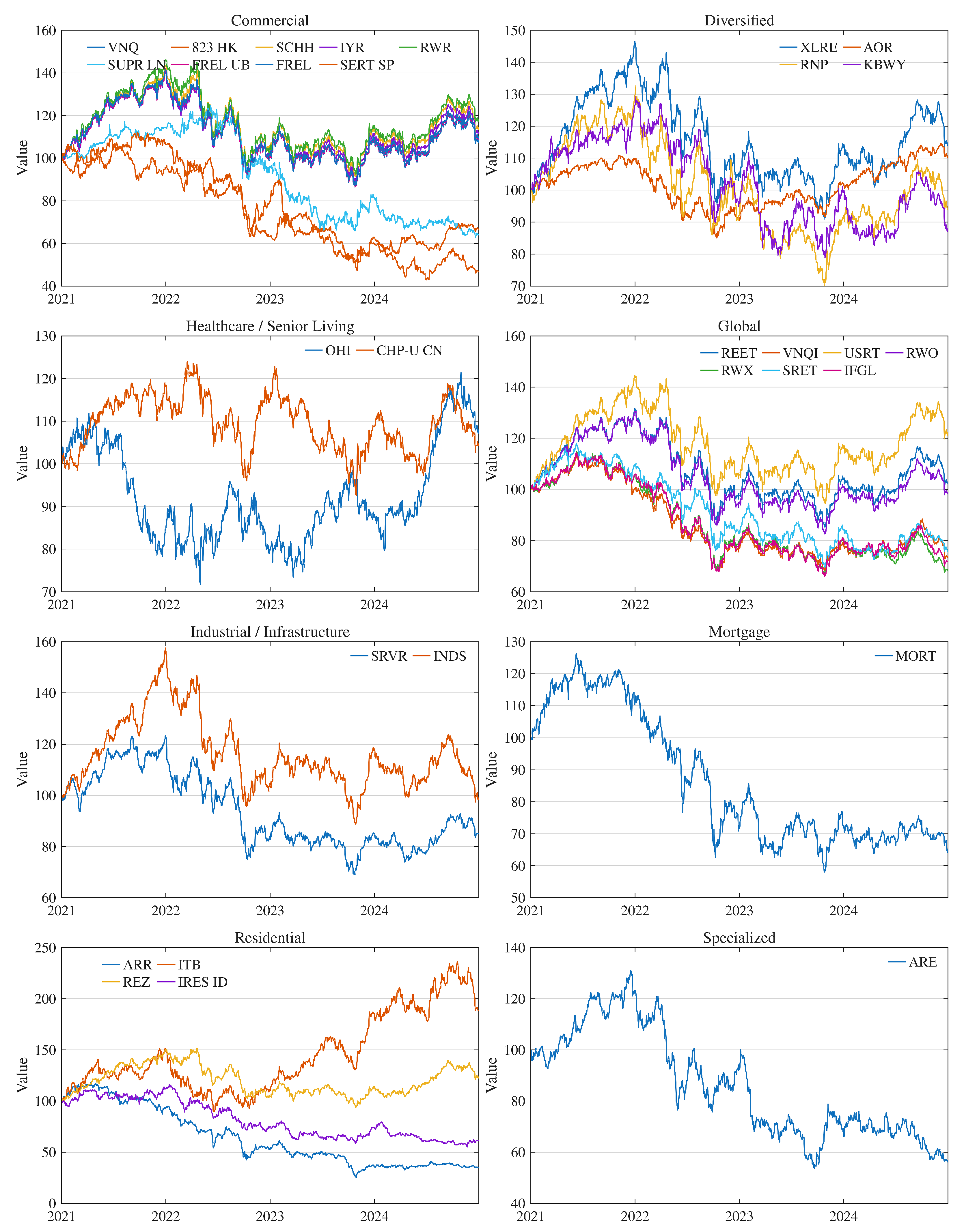
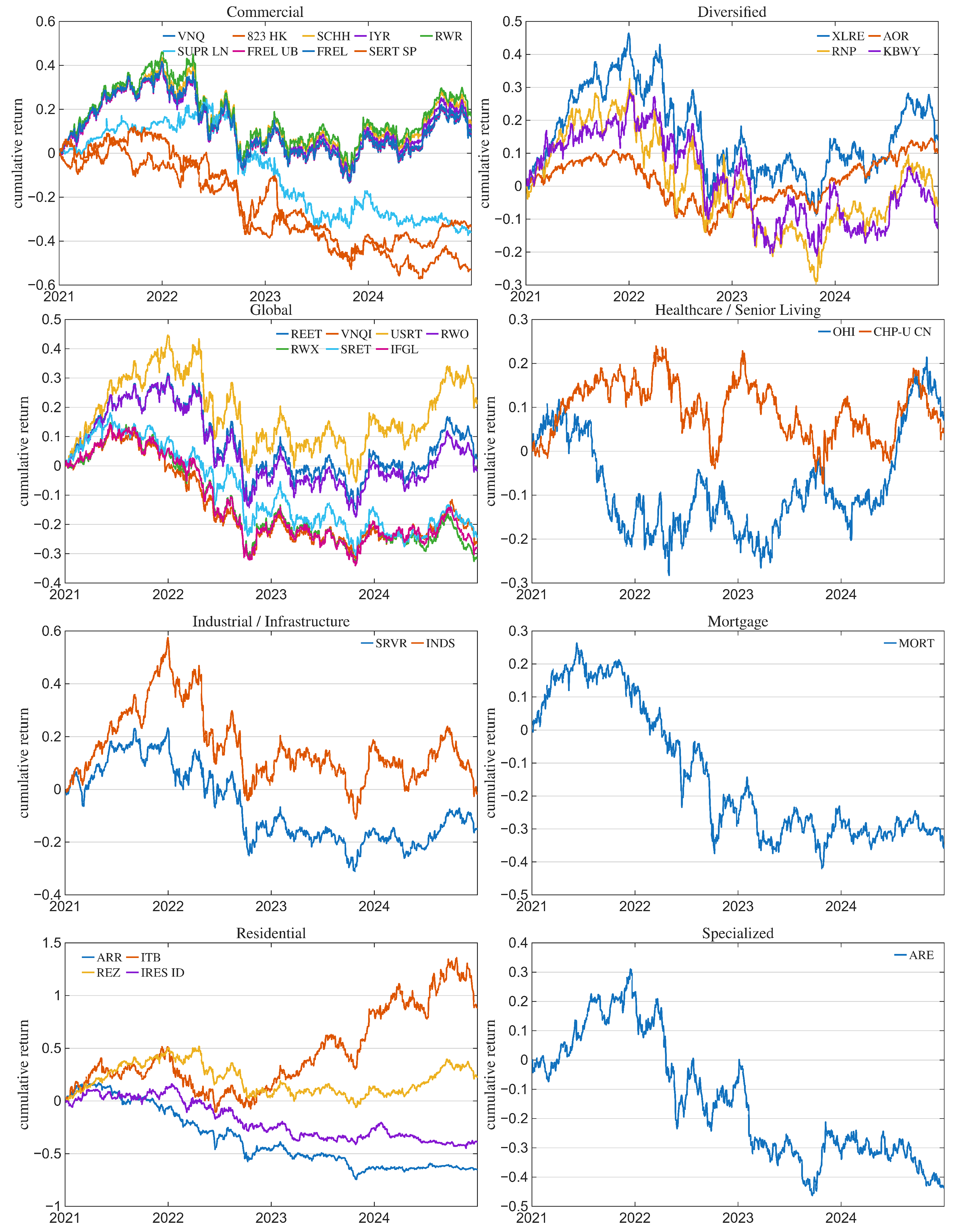
Section 2 describes the security universe of 30 U.S. and international real estate securities used in our study. Performance of the individual securities is compared by value and cumulative return.

We examined the comparative performance of historical optimization using long-only and long–short strategies under variance (Markowitz) and downside-risk (CVaR)-based optimizations. We considered the minimum-risk and tangent portfolios from each respective efficient frontier. Section 3 compares the relative value performance of the strategy-optimized portfolios. Examples of efficient frontiers for two dates during the study period are also provided.

We assessed the tail behavior of the distributions of optimized return series over the study period via skewness and kurtosis and the application of extreme value theory to determine the heaviness of the lower (loss) and upper (gain) tails. Section 4 presents the results of this analysis. Section 5 complements this analysis, presenting the results of selected risk-adjusted performance measures, including reward/risk ratios, for the strategy-optimized portfolios.

We examined persistence (long-range dependence) in the conditional mean and volatility of the optimized return series through ARFIMA–GARCH and ARMA–FIGARCH models (Baillie, 1996; Bollerslev, 1986). Section 6 discusses the model and parameter choices and presents the results of the fits.

We employed the CAPM to measure the extent to which the portfolio returns were explained by endogenous and exogenous market proxies. As an endogenous proxy, we used a buy-and-hold portfolio consisting of the 30 real estate securities; the Dow Jones Industrial Average was used as the exogenous proxy. To guard against outlier influence, we employed robust regression (Maronna et al., 2019; Rousseeuw & Leroy, 2003; Yohai, 1987) to obtain the CAPM parameters. Section 7 presents the results of the CAPM analyses.

We calibrated a normal double-inverse Gaussian (NDIG) subordinated option-pricing model to obtain option prices based, respectively, on each optimized portfolio as underlying. NDIG was employed as it has been shown that single subordination fails to explain the equity premium problem (Lundtofte & Wilhelmsson, 2013; Shirvani et al., 2021). NDIG retains the flexibility to capture non-Gaussian effects in return distributions. Section 8 briefly summarizes the NDIG option-pricing method. Example call price surfaces are presented and compared against prices computed using the Black–Scholes formula. Corresponding implied volatility surfaces are also computed from the NDIG model.

Section 9 presents a summary discussion of the work.

2. Data and Descriptive Statistics

Data Description

The sample consisted of 30 actively traded, real estate securities spanning domestic, worldwide, and regional funds in eight sectors. Daily adjusted closing price and market capitalization data for the period 4 January 2021 to 31 December 2024 were obtained from Bloomberg Professional Services.1 This period covers the post-pandemic recovery, the 2022 interest-rate tightening cycle, and the subsequent repricing of U.S. and global property markets.

Table A1. Real estate securities included in this study, categorized by sector and market capitalization as of 30 January 2025.

BBG Ticker	Name	Inception Date	Market Cap (Million)	Exchange
	Commercial
VNQ	Vanguard Real Estate ETF	9/29/2004	33,890 USD	NYSE Arca
823 HK	Link REIT	9/6/2005	108,461 HKD	HKEX
SCHH	Schwab U.S. REIT ETF	1/13/2011	7990 USD	NYSE Arca
IYR	iShares U.S. Real Estate ETF	6/19/2000	3760 USD	NYSE Arca
RWR	SPDR Dow Jones REIT ETF	4/27/2001	2030 USD	NYSE Arca
SUPR LN	Supermarket Income REIT plc	21/7/2017	1041 GBP	LSE
FREL US a	Fidelity MSCI Real Estate Index ETF	2/5/2015	1060 USD	NYSE Arca
FREL UB a	Fidelity MSCI Real Estate Index ETF	2/5/2015	1060 USD	BBG: US Composite
SERT SP	Sasseur REIT	30/10/2017	886 EUR	SGX
	Diversified
XLRE	Real Estate Select Sector SPDR Fund	10/8/2015	7490 USD	NYSE Arca
AOR	iShares Core 60/40 Balanced Allocation ETF	11/11/2008	2410 USD	NYSE Arca
RNP	Cohen & Steers REIT & Preferred and Income Fund	6/27/2003	1040 USD	NYSE
KBWY	Invesco KBW Premium Yield Equity REIT ETF	12/2/2010	224 USD	NASDAQ
	Global
REET	iShares Global REIT ETF	7/10/2014	3950 USD	NYSE Arca
VNQI	Vanguard Global ex-U.S. Real Estate ETF	11/1/2010	3320 USD	NASDAQ
USRT	iShares Core U.S. REIT ETF	5/4/2007	2990 USD	NYSE Arca
RWO	SPDR Dow Jones Global Real Estate ETF	5/13/2008	1120 USD	NYSE Arca
RWX	SPDR Dow Jones International Real Estate ETF	12/15/2006	382 USD	NYSE Arca
SRET	Global X SuperDividend REIT ETF	3/16/2015	183 USD	NASDAQ
IFGL	iShares International Developed Real Estate ETF	11/19/2007	92 USD	NASDAQ
	Healthcare/Senior Living
OHI	Omega Healthcare Investors, Inc. (Hunt Valley, MD, USA)	31/3/1992	10,713 USD	NYSE
CHP-U CN	Chartwell Retirement Residences	14/11/2003	10,461 CAD	TSX
	Industrial/Infrastructure
SRVR	Pacer Data & Infrastructure Real Estate ETF	5/16/2018	445 USD	NYSE Arca
INDS	Pacer Industrial Real Estate ETF	5/15/2018	141 USD	NYSE Arca
	Mortgage
MORT	VanEck Mortgage REIT Income ETF	8/17/2011	302 USD	NYSE Arca
	Residential
ITB	iShares U.S. Home Construction ETF	5/5/2006	2140 USD	NYSE Arca
ARR	ARMOUR Residential REIT, Inc. (Vero Beach, FL, USA)	5/2/2008	1374 USD	NYSE
REZ	iShares Residential and Multi-sector Real Estate ETF	5/4/2007	795 USD	NASDAQ
IRES ID	Irish Residential Properties REIT plc	16/4/2014	565 EUR	Euronext Dublin
	Specialized
ARE	Alexandria Real Estate Equities, Inc. (Pasadena, CA, USA)	27/3/1997	12,661 USD	NYSE

^a Data differences between FREL US and FREL UB are minor. FREL UB was included for diagnostic purposes.

in Appendix A summarizes the selected instruments by ticker, fund name, inception date, and market capitalization.

Figure 1 reports the value of a 100 USD buy-and-hold position in each real estate security over the sample period. The panels show that the 2022 tightening cycle affected most funds, with subsequent performance differing both within and across segments. Figure A1 (Appendix B) reports the corresponding cumulative arithmetic returns of the values displayed in Figure 1.

To document broader equity-market conditions, we used the Dow Jones Industrial Average (DJIA) as an external benchmark.2 The choice of the DJIA was based on the following. We recognize that a possible choice would have been a real estate-specific index (e.g., MSCI World Real Estate Index). However, our interest is the view of a multi-sector investor, for which real estate investment is one possible sector of interest. For general market indices, the S&P 500 or Russell 3000 would be possible candidates; the Dow was chosen due to its ubiquitous use. As a minor coincidence, the DJIA is based upon the same number of assets as our real estate security universe.

The three-month U.S. Treasury bill rate (converted to a daily rate) was used as the short-term risk-free proxy.3 We note that arithmetic returns were used for all computations in Section 3, Section 4, Section 5, Section 6 and Section 7, while log-returns were used in Section 8.

3. Portfolio Optimization

We examined historical portfolio strategies under mean–variance and CVaR risk measures. Mean–variance optimization minimizes portfolio return variance for a targeted return, whereas CVaR optimization minimizes expected loss for a targeted return. We report separate CVaR optimizations at 95% and 99% confidence levels. All portfolio weights were estimated using a rolling window of 504 days. This produced optimized returns for the time period 12 December 2022 to 31 December 2024. We refer to this as the study period.

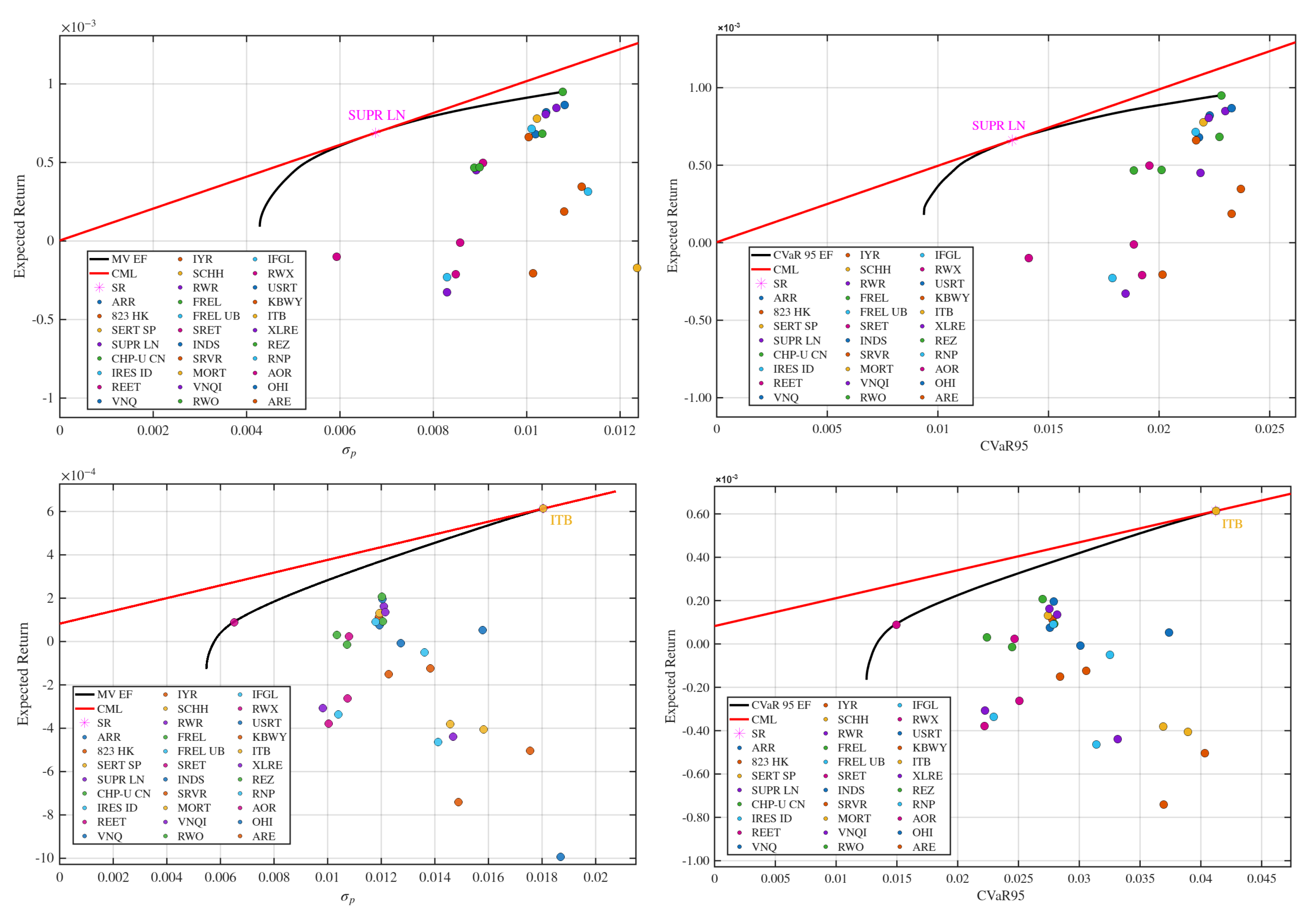
Figure 2 reports the mean–variance and CVaR95-efficient frontiers, the corresponding capital market lines, and individual security mean returns computed for two dates, 29 April 2022 and 31 December 2024. The April 2022 date falls within the monetary tightening cycle, when rising interest rates and repricing pressure weighed heavily on the real estate sector. For the December 2024 date, on both efficient frontiers, the tangent portfolio lies close to the ETF ITB, indicating that ITB had a substantial influence on the tangent allocation on that date.

We considered two investment strategies: long-only and long–short. The long-only strategy imposed the usual constraints

$$0\le w_i\left(t_k\right)\le 1,\sum _i{w}_i\left(t_k\right)=1,$$

where $w_i\left(t_k\right)$ denotes the weight assigned to asset i over the holding period $[t_k,t_{k+1})$. Our long–short strategy relaxed the bounds to

$$-w_{\mathrm{lev}}\le w_i\left(t_k\right)\le 1+w_{\mathrm{lev}},w_{\mathrm{lev}}={\displaystyle \frac{1}{30}},\sum _i{w}_i\left(t_k\right)=1,$$

The choice $w_{\mathrm{lev}}=1/30$ restricted the short position in any one security to no more than its allocation within an equally weighted portfolio.

Under both strategies, portfolio rebalancing was governed by the turnover constraint

$${\displaystyle \frac{1}{2}}{\displaystyle \sum _{i=1}^{30}}\left|w_i\left(t_k\right)-w_i\left(t_{k-1}\right)\right|<C_{\mathrm{TO}}.$$

We set

$$C_{\mathrm{TO}}={\displaystyle \frac{1}{30·252}}\approx 1.3228\times {10}^{-4}$$

at each rebalance date. The choice of the value for $C_{\mathrm{TO}}$ restricted the total annual weight turnover of the portfolio to less than 100%.

For each optimization type, we report two portfolios on the efficient frontier, the minimum-risk and tangent portfolios. For brevity, we refer to the strategy-optimized portfolios as

• LO MVP long-only, mean–variance, minimum-risk portfolio;
• LO TVP long-only, mean–variance, tangent portfolio;
• LO C95 long-only, CVaR95, minimum-risk portfolio;
• LO TC95 long-only, CVaR95, tangent portfolio;
• LO C99 long-only, CVaR99, minimum-risk portfolio;
• LO TC99 long-only, CVaR99, tangent portfolio.

The same notation, with LO replaced by LS, is used for the corresponding long–short strategy-optimized portfolios.

As an endogenous benchmark, we modeled a passive buy-and-hold portfolio (BHP) initialized with equal weights across the 30 securities. The BHP was not rebalanced; its weights changed over time under relative asset performance. Hence, the BHP became differentially concentrated in those assets that performed best in different time periods (Forsyth, 2024).

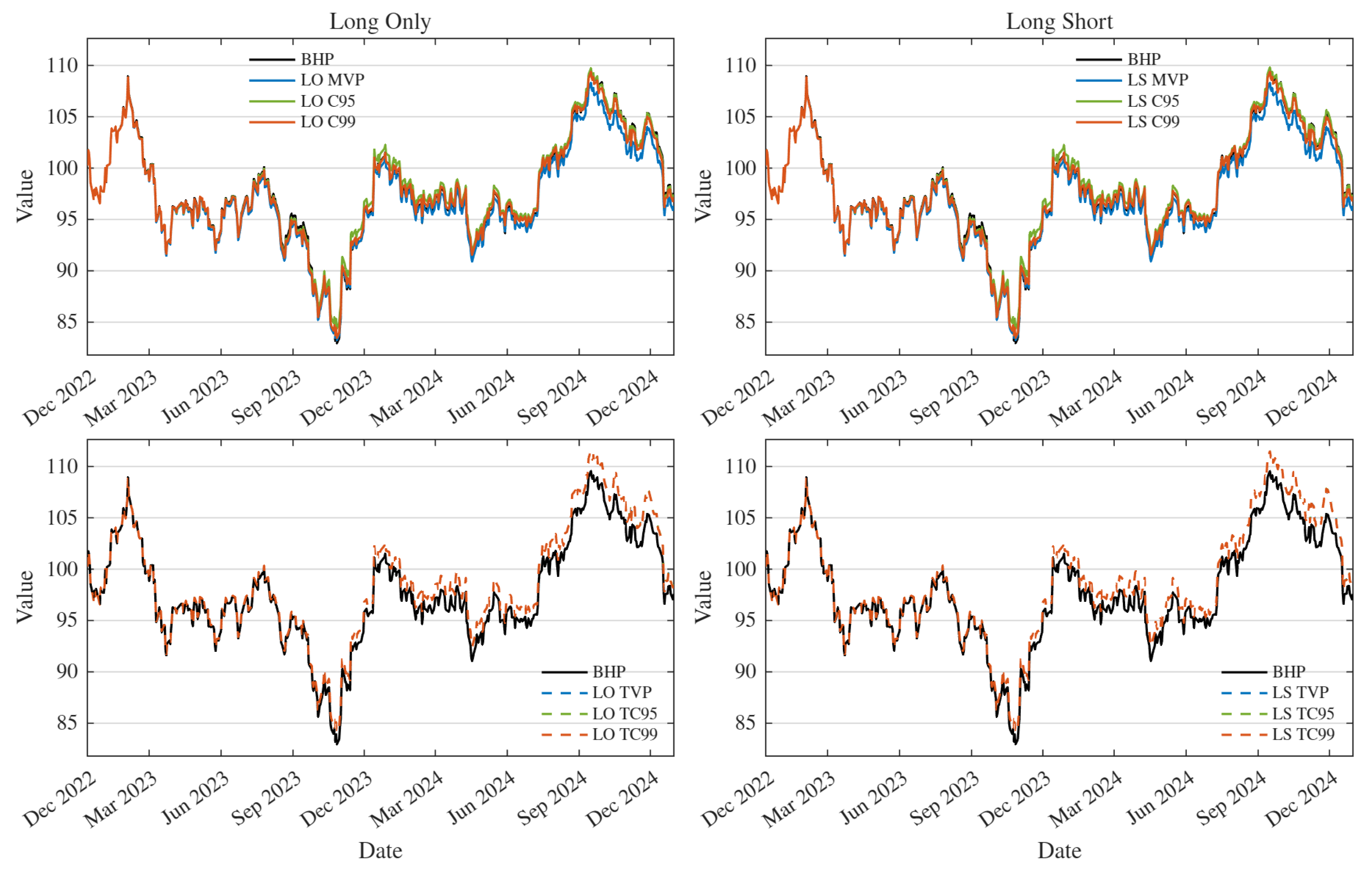
Figure 3 reports portfolio values based on an initial 100 USD investment. Prior to mid-2023, the optimized portfolio values remained close to the BHP. After mid-2023, LO MVP and LS MVP remained below the BHP, while the other minimum-risk portfolios remained close to the BHP. In contrast, after mid-2023, all tangent portfolios outperformed the BHP.

4. Tail Behavior

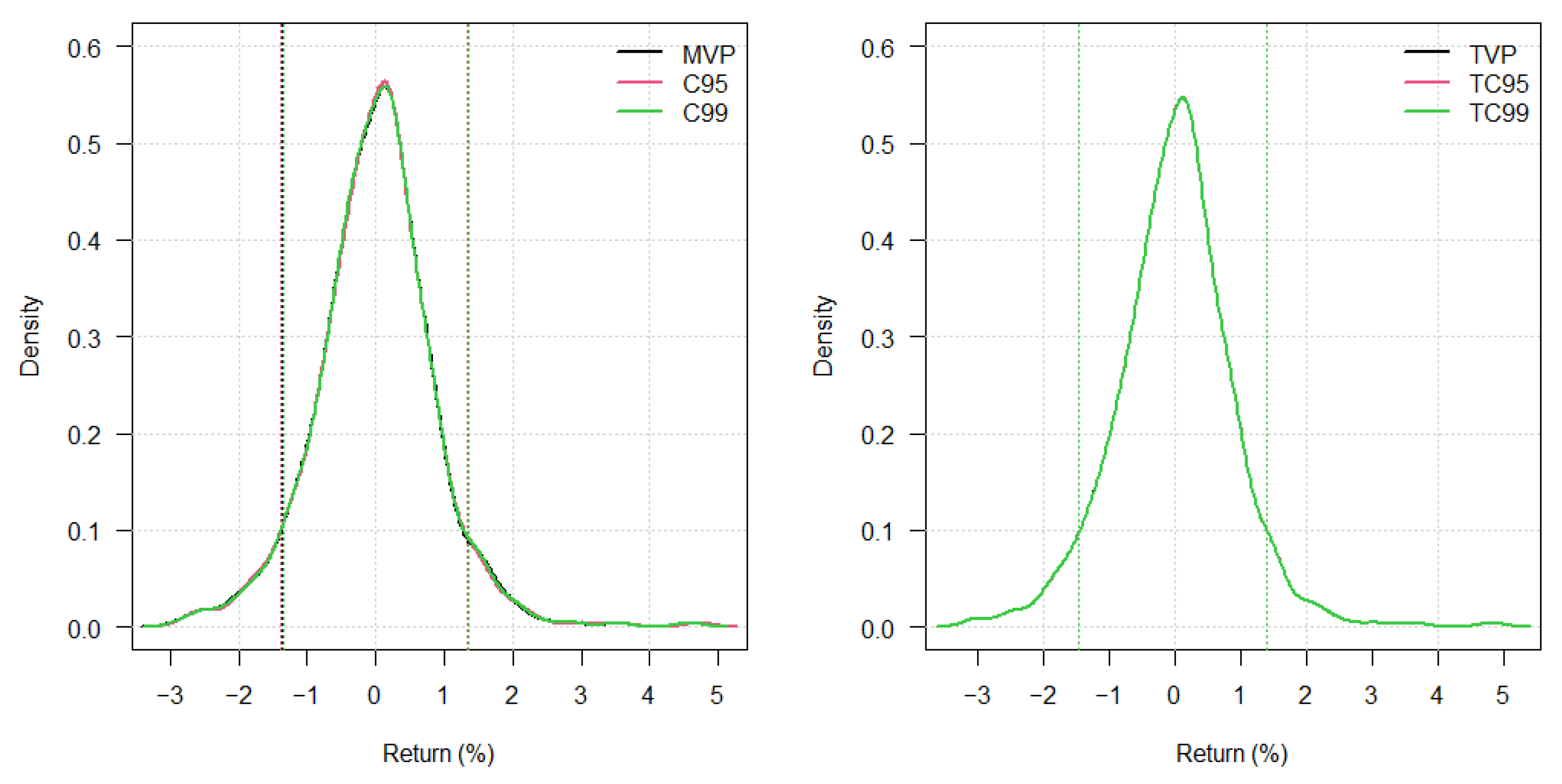
We address the impact of strategy-optimized portfolio choice on the tail behavior of returns. Figure 4 presents the kernel density plots of the long-only optimized minimum-risk and tangent portfolio distributions of returns over the study period. The distributions are remarkably visually similar (and equally similar to the long–short strategy optimizations). The mean values of the distributions were in the range $[-3.46·{10}^{-3},-1.28·{10}^{-3}]$ percent, whereas modal values were approximately $0.14$ percent.

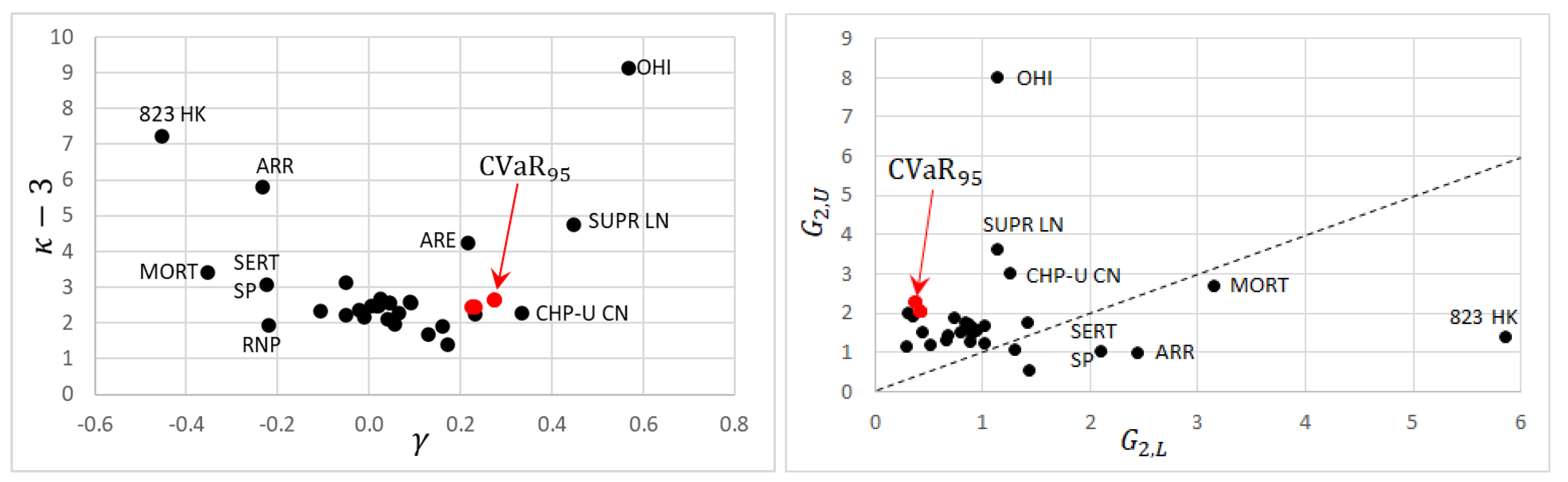
Focusing on tail behavior, Figure 5 plots the values $(\gamma ,\kappa -3)$, where $\gamma$ is the skewness and $\kappa -3$ is the excess kurtosis, for the distribution of returns of the individual securities and strategy-optimized portfolios over the study period. There is a substantial difference in skewness and excess kurtosis between the individual securities. The securities with “outlying” values are identified. In contrast, the $(\gamma ,\kappa -3)$ values for the 12 optimized portfolios were clustered into two tight regions. The four portfolios optimized under CVaR 95% comprised one cluster (identified by arrow in the figure) and the remaining eight comprised the second cluster. The optimized portfolios all had positive skewness $\gamma \in [0.225,0.272]$ and excess kurtosis values $\kappa -3\in [2.470,2.662]$ in narrow ranges.

Given a return series $R_t$, $t=1,\dots ,T$, an unbiased sample estimator for the excess kurtosis is

$$\begin{array}{cc}\hfill G_2& ={\displaystyle \frac{T-1}{(T-2)(T-3)}}\left[(T+1)g_2+6\right],\hfill \\ \hfill g_2& ={\displaystyle \frac{1}{T}}{\displaystyle \sum _{t=1}^T}{z}_t^2-3,z_t={\displaystyle \frac{R_t-\overline{R}}{{\sigma }_b}},\hfill \end{array}$$

where

$${\sigma }_b^2={\displaystyle \frac{1}{T}}{\displaystyle \sum _{t=1}^T}{(R_t-\overline{R})}^2\mathrm{and}\overline{R}={\displaystyle \frac{1}{T}}{\displaystyle \sum _{t=1}^T}{R}_t,$$

are, respectively, the biased sample variance and unbiased sample mean estimators. Defining

$$g_{2,\mathrm{L}}={\displaystyle \frac{1}{T}}\sum _{z_t\le 0}{z}_t^2-1.5,g_{2,\mathrm{U}}={\displaystyle \frac{1}{T}}\sum _{z_t>0}{z}_t^2-1.5,$$

we can compute the components of excess kurtosis

$$G_{2,\mathrm{L}}={\displaystyle \frac{T-1}{(T-2)(T-3)}}\left[(T+1)g_{2,\mathrm{L}}+3\right],G_{2,\mathrm{U}}={\displaystyle \frac{T-1}{(T-2)(T-3)}}\left[(T+1)g_{2,\mathrm{U}}+3\right],$$

coming from the lower and upper (relative to the mean) parts of the distribution. (Note that $G_2=G_{2,\mathrm{L}}+G_{2,\mathrm{U}}$.) Figure 5 plots the values $(G_{2,\mathrm{L}},G_{2,\mathrm{U}})$ for the distribution of returns of the individual securities and strategy-optimized portfolios over the study period. Six of the securities have dominant lower-tail excess kurtosis; the rest, including the optimized portfolios, have dominant upper-tail excess kurtosis.

While centered $p-$moments increasingly weight the tail regions as p increases, moment computations are still influenced by the central portion of the distribution. We therefore targeted the tail regions using extreme value theory. We define a heavy-tailed distribution $f\left(x\right)$ (sometimes equivalently, and other times distinctly, referred to as a fat-tailed distribution) as a distribution that exhibits large skewness or excess kurtosis, and which, for large x, goes to zero as $x^{-\alpha }$. The value $\alpha$ is referred to as the tail index.

We estimated the upper-tail index $\alpha$ using the non-parametric estimator of Hill (1975). Let $U_1,\dots ,U_m$ denote a sample of positive returns arranged in descending order, $U_1\ge U_2\ge \cdots \ge U_m$, where m is determined by some threshold tail value. For the largest $k\le m$ observations, the Hill estimator of the tail index $\alpha$ is

$${\alpha }_{k,m}^{\left(H\right)}={\left({\displaystyle \frac{1}{k}}{\displaystyle \sum _{i=1}^k}\log {\displaystyle \frac{U_i}{U_{k+1}}}\right)}^{-1}.$$

(1)

(To examine the lower tail of a return distribution sample $\left\{R_j\right\}$, define the loss values $L_j=-R_j$ and apply the Hill estimator to the upper tail of the loss distribution.)

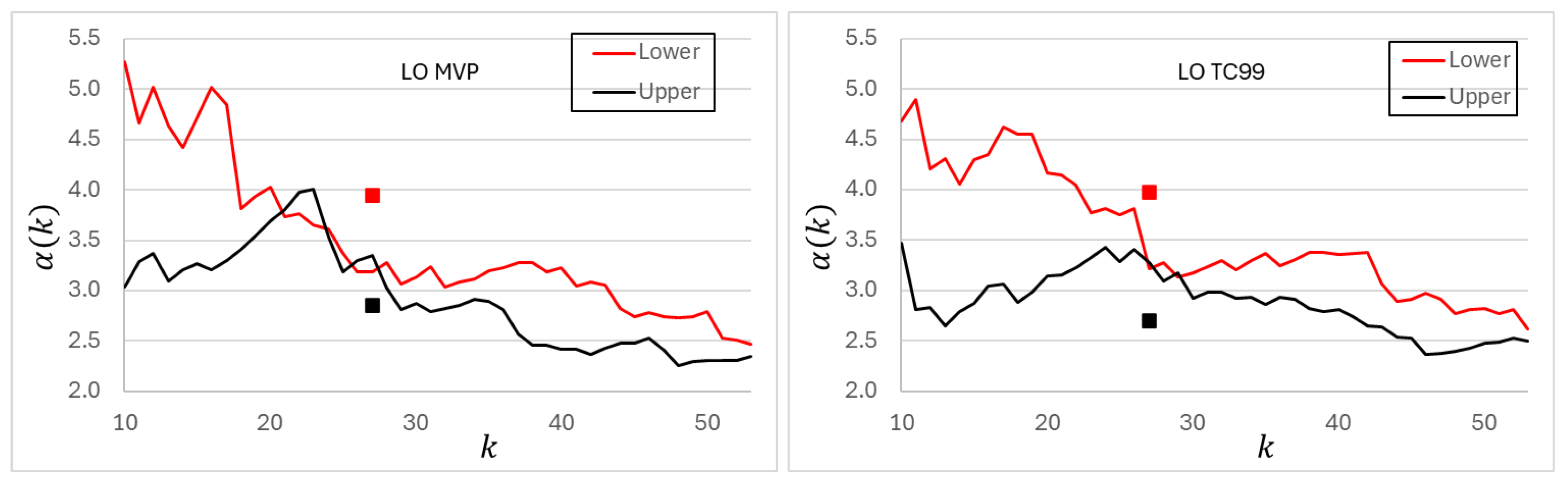
Figure 6 presents the Hill estimates of the tail index $\alpha \left(k\right)$ for $k\in [10,53]$ for the lower and upper tails of the return series of LO MVP and LO TC99. The range of k values corresponds to using the return distribution percentile ranges [1.89, 10.0] and [90, 98.01] to define the lower- and upper-tail regions, respectively. Using the Hill estimator, the choice of a single tail-representative value of $\alpha$ is k-dependent. Various procedures (e.g., de Sousa & Michailidis, 2004) have been proposed to choose the “best” k value for the Hill estimator. Our interest is to determine the range of k values estimated over a reasonable region of the tail (avoiding, unfortunately, the most interesting extreme region $k<10$ of the tail due to poor sample statistics).

The results for LO MVP and LO TC99 are representative of the other 10 strategy-optimized portfolios. Generally, at a given value of k, $\alpha \left(k\right)$ for the lower tail exceeded that for the upper tail. Lower-tail values of $\alpha \left(k\right)$ ranged over [2.5, 5.5], while those for the upper tail ranged over [2.3, 4.0]. The closest agreement between $\alpha \left(k\right)$ values for the two tails occurred within the range $20<k<30$.

We supplemented the Hill estimates with Pareto log–log survival diagnostics of the kernel density distributions computed for the strategy-optimized portfolio return series. Let

$$\overline{F}\left(x\right)=P(L>x\mid L>x_m)$$

denote the survival function above a tail threshold value $x_m>0$. Under a Pareto distribution approximation,

$$\overline{F}\left(x\right)\approx {\left({\displaystyle \frac{x_m}{x}}\right)}^{\alpha },x\ge x_m.$$

(2)

If the upper (or lower) tail of the kernel density is approximately Pareto over the range $x\ge x_m$, then a plot of $\log \overline{F}\left(x\right)$ against $\log x$ should be approximately linear with slope $-\alpha$.

Table A2. Fitted log–log survival fit parameter and goodness-of-fit values for the lower and upper tails of the return distributions for the strategy-optimized portfolios.

Portfolio	Lower Tail			Upper Tail
	α	SEα	${\mathit{R}}^2$	α	SEα	${\mathit{R}}^2$
LO MVP	3.956	0.198	0.941	2.859	0.087	0.977
LO C95	4.033	0.192	0.946	2.744	0.071	0.984
LO C99	3.920	0.194	0.942	2.834	0.078	0.981
LO TVP	3.978	0.138	0.971	2.708	0.062	0.987
LO TC95	3.978	0.138	0.971	2.708	0.062	0.987
LO TC99	3.978	0.138	0.971	2.708	0.062	0.987
LS MVP	3.956	0.198	0.941	2.859	0.087	0.977
LS C95	4.047	0.196	0.945	2.736	0.068	0.985
LS C99	3.909	0.191	0.943	2.838	0.080	0.981
LS TVP	4.014	0.145	0.968	2.704	0.063	0.987
LS TC95	4.024	0.145	0.968	2.704	0.063	0.987
LS TC99	4.022	0.145	0.968	2.703	0.063	0.987

SE: standard error.

(Appendix C) presents the resultant log–log survival fits for $\alpha$ for the lower and upper tails of the strategy-optimized portfolios for the values of $x_m$ corresponding to the lower and upper 5% of return values. The standard error and $R^2$ values indicate that the linear fit supposition was very good. The square points in Figure 6 show the values obtained from these log–log survival fits for the tail regions of LO MVP and LO TC99. The log–log survival plots are in good agreement with the range of $\alpha$ values obtained from the Hill estimator. This observation is true for the remaining 10 strategy-optimized portfolios.

5. Risk Metrics

We analyzed the historical performance of the optimized portfolios using a set of standard risk-adjusted measures: volatility, maximum drawdown, and the Sharpe, Sortino, Rachev,4 and information5 ratios. These measures variously address overall dispersion, drawdown severity, downside risk, tail asymmetry, and benchmark-relative performance.

Table 1. Risk measure values ordered by increasing Sharpe ratio.

Portfolio	Vol a (×10−3)	MDD b	Sharpe Ratio	Sortino Ratio	Rachev Ratio	IR c
LO MVP	8.50	0.235	−0.360	−0.351	0.998	−0.501
LS MVP	8.50	0.235	−0.360	−0.351	0.998	−0.501
LO C99	8.50	0.233	−0.329	−0.323	1.002	−0.211
LS C99	8.50	0.233	−0.326	−0.321	1.002	−0.186
LS C95	8.57	0.225	−0.319	−0.314	1.012	−0.120
LO C95	8.50	0.225	−0.319	−0.313	1.010	−0.116
BHP	8.82	0.239	−0.297	−0.289	0.989	NA
LO TC99	8.88	0.228	−0.255	−0.249	0.998	0.643
LS TC99	8.88	0.228	−0.254	−0.248	1.000	0.666
LS TC95	8.88	0.228	−0.253	−0.247	1.001	0.675
LS TVP	8.88	0.228	−0.253	−0.247	1.001	0.685
LO TVP	8.88	0.228	−0.253	−0.248	0.998	0.663
LO TC95	8.88	0.228	−0.253	−0.248	0.998	0.662

^a Vol: volatility; ^b MDD: maximum drawdown; ^c IR: information ratio; NA: not applicable.

reports estimates of the performance measures computed from the optimized portfolio return series over the study period. The Sharpe, Sortino, and information ratios reflect distinct performance differences between the minimum-risk and tangent portfolios: Sharpe ([$-0.360,-0.319$] versus [$-0.255,-0.253$]); Sortino ([$-0.351,-0.313$] versus [$-0.249,-0.247$]); IR ([$-0.501,-0.116$] versus [$0.643, 0.685$]). The difference was present, but less distinct, in the volatility ([0.00850, 0.00857] versus [0.00888, 0.00888]). The BHP had the greatest maximum drawdown. The Rachev ratios were close to one for the optimized portfolios, suggesting that the estimated upper-tail to lower-tail trade-off was broadly similar across the optimization strategies. With limited overlap, the Rachev ratios tended to be slightly higher for the minimum-risk portfolios ([0.998, 1.012] versus [0.998, 1.001]). For each measure, there was more variation in value among the minimum-risk portfolios than among the tangent portfolios. There appeared to be a negligible difference between the long-only and long–short versions of the same optimized portfolio.

We characterized the loss (negative return = positive loss) tail of the optimized return series using VaR95, CVaR95, VaR99, and CVaR99 values.

Table 2. Tail-loss measures for all portfolio strategies. The portfolios are listed in order of increasing value of VaR95.

Portfolio	VaR0.95	CVaR0.95	VaR0.99	CVaR0.99
LO C99	0.0136	0.0189	0.0225	0.0259
LS C99	0.0136	0.0189	0.0225	0.0259
LS MVP	0.0137	0.0190	0.0225	0.0260
LO MVP	0.0137	0.0190	0.0225	0.0260
LO C95	0.0140	0.0189	0.0225	0.0259
LS C95	0.0140	0.0188	0.0225	0.0259
BHP	0.0149	0.0197	0.0241	0.0271
LS TC95	0.0149	0.0196	0.0241	0.0271
LS TC99	0.0149	0.0196	0.0241	0.0271
LS TVP	0.0149	0.0196	0.0241	0.0271
LO TVP	0.0149	0.0196	0.0243	0.0273
LO TC95	0.0149	0.0196	0.0243	0.0273
LO TC99	0.0149	0.0196	0.0243	0.0273

reports these values for all portfolios. Befitting their definition, the minimum-risk portfolios record the smallest tail-loss measures. What is perhaps surprising is the relative similarity in any particular value for the different minimum-risk portfolios. The same observation holds for the tangent portfolios. The passive BHP attained values comparable to the tangent portfolios.

6. Long-Range Dependence in Conditional Mean and Variance

Testing for long-range dependence (LRD) in a time series using ARFIMA–FIGARCH models with specification of the distribution for the innovations is an elusive process. Experience has shown that specifying a heavy-tailed distribution (e.g., $t-$distribution) for the innovations tends to mask any LRD dependence in the conditional variance and mean. If a “light-tailed” distribution (e.g., normal or exponential) is used with ARFIMA–FIGARCH, any LRD in the volatility tends to be so strong as to mask any LRD in the mean. A compromise is to test separate ARFIMA–GARCH–normal and ARMA–FIGARCH–normal models to attempt some measure of LRD in the mean and volatility.

To test for LRD in the conditional mean, we fitted an ARFIMA($m,d,n$)–GARCH(1,1)–normal model to the study period return series of the optimized portfolios:

$$\begin{array}{cc}\hfill & (1-{\displaystyle \sum _{j=1}^{m_i}}{\varphi }_{i,j}{L}^j){(1-L)}^{d_i}(R_{i,t}-{\mu }_i)=(1-{\displaystyle \sum _{k=1}^{n_i}}{\theta }_{i,k}{L}^k){\epsilon }_{i,t},\hfill \\ \hfill & {\epsilon }_{i,t}=z_{i,t}\sqrt{h_{i,t}},z_{i,t}\sim \mathcal{N}(0,1),\hfill \\ \hfill & h_{i,t}={\omega }_i+{\alpha }_i{\epsilon }_{i,t-1}^2+{\beta }_i{h}_{i,t-1}.\hfill \end{array}$$

(3)

where L is the lag operator, $h_{i,t}$ is the conditional variance for portfolio i, and $d_i$ is the fractional differencing parameter for the conditional mean. For each portfolio i, the orders $m_i$ and $n_i$ were selected from the possibilities $m_i,n_i\in \{0,\dots ,3\}$ by requiring that the AR and MA coefficients ${\varphi }_{i,j}$, $j=1,\dots ,m_i$, and ${\theta }_{i,k}$, $k=1,\dots ,n_i$, have significant p-values. The choice $m_i,n_i$ corresponding to the lowest BIC value among the p-value significant solutions was selected.

For the optimized portfolios, the selected conditional-mean specification was ARFIMA(2,d,2). The parameter estimates and corresponding p-values for the ARFIMA(2,d,2)–GARCH(1,1) fit are reported in

Table A3. ARFIMA(2,d,2)-GARCH(1,1) parameter estimates for the indicated optimized portfolio return series. Numbers in parentheses indicate p-values.

Portfolio $\mathit{i}$	${\mathit{\mu }}_{\mathit{i}}$ (×10−4)	${\mathit{\varphi }}_{\mathit{i},1}$	${\mathit{\varphi }}_{\mathit{i},2}$	${\mathit{\theta }}_{\mathit{i},1}$	${\mathit{\theta }}_{\mathit{i},2}$	${\mathit{d}}_{\mathit{i}}$	${\mathit{\omega }}_{\mathit{i}}$ (×10−4)	${\mathit{\alpha }}_{\mathit{i}}$	${\mathit{\beta }}_{\mathit{i}}$
LO MVP	$-1.765$	$0.1740$	$-0.9925$	$-0.1943$	$0.9964$	$0.0704$	$1.204$	$0.0312$	$0.9508$
	$\left(0.7391\right)$	(****)	(****)	(****)	(****)	$\left(0.0626\right)$	$\left(0.1185\right)$	$\left(0.0066\right)$	(****)
LS MVP	$-1.766$	$0.1740$	$-0.9925$	$-0.1943$	$0.9964$	$0.0704$	$1.204$	$0.0312$	$0.9508$
	$\left(0.7390\right)$	(****)	(****)	(****)	(****)	$\left(0.0626\right)$	$\left(0.1185\right)$	$\left(0.0066\right)$	(****)
LO TVP	$-1.250$	$0.1734$	$-0.9926$	$-0.1950$	$0.9970$	$0.0649$	$2.060$	$0.0234$	$0.9490$
	$\left(0.8186\right)$	(****)	(****)	(****)	(****)	$\left(0.0858\right)$	$\left(0.1000\right)$	$\left(0.0214\right)$	(****)
LS TVP	$-1.250$	$0.1734$	$-0.9927$	$-0.1948$	$0.9970$	$0.0664$	$1.987$	$0.0240$	$0.9491$
	$\left(0.8193\right)$	(****)	(****)	(****)	(****)	$\left(0.0791\right)$	$\left(0.0976\right)$	$\left(0.0190\right)$	(****)
LO C95	$-1.622$	$0.1743$	$-0.9928$	$-0.1945$	$0.9969$	$0.0728$	$1.212$	$0.0297$	$0.9522$
	$\left(0.7638\right)$	(****)	(****)	(****)	(****)	$\left(0.0540\right)$	$\left(0.1143\right)$	$\left(0.0064\right)$	(****)
LS C95	$-1.587$	$0.1744$	$-0.9930$	$-0.1942$	$0.9971$	$0.0733$	$1.240$	$0.0294$	$0.9522$
	$\left(0.7697\right)$	(****)	(****)	(****)	(****)	$\left(0.0526\right)$	$\left(0.1100\right)$	$\left(0.0066\right)$	(****)
LO C99	$-1.637$	$0.1738$	$-0.9928$	$-0.1939$	$0.9965$	$0.0729$	$1.218$	$0.0298$	$0.9520$
	$\left(0.7612\right)$	(****)	(****)	(****)	(****)	$\left(0.0537\right)$	$\left(0.1157\right)$	$\left(0.0067\right)$	(****)
LS C99	$-1.641$	$0.1737$	$-0.9927$	$-0.1940$	$0.9964$	$0.0727$	$1.214$	$0.0299$	$0.9519$
	$\left(0.7604\right)$	(****)	(****)	(****)	(****)	$\left(0.0543\right)$	$\left(0.1177\right)$	$\left(0.0068\right)$	(****)
LO TC95	$-1.248$	$0.1734$	$-0.9926$	$-0.1950$	$0.9970$	$0.0649$	$2.062$	$0.0234$	$0.9490$
	$\left(0.8188\right)$	(****)	(****)	(****)	(****)	$\left(0.0860\right)$	$\left(0.1000\right)$	$\left(0.0214\right)$	(****)
LS TC95	$-1.259$	$0.1734$	$-0.9927$	$-0.1948$	$0.9970$	$0.0665$	$1.983$	$0.0241$	$0.9491$
	$\left(0.8182\right)$	(****)	(****)	(****)	(****)	$\left(0.0785\right)$	$\left(0.0979\right)$	$\left(0.0190\right)$	(****)
LO TC99	$-1.257$	$0.1734$	$-0.9926$	$-0.1950$	$0.9970$	$0.0649$	$2.066$	$0.0234$	$0.9490$
	$\left(0.8176\right)$	(****)	(****)	(****)	(****)	$\left(0.0857\right)$	$\left(0.1000\right)$	$\left(0.0214\right)$	(****)
LS TC99	$-1.262$	$0.1734$	$-0.9927$	$-0.1948$	$0.9970$	$0.0665$	$1.986$	$0.0241$	$0.9491$
	$\left(0.8178\right)$	(****)	(****)	(****)	(****)	$\left(0.0785\right)$	$\left(0.0979\right)$	$\left(0.0190\right)$	(****)

(****) indicates a p-value less than ${10}^{-4}$.

in Appendix D. The parameters ${\varphi }_{i,1}$, ${\varphi }_{i,2}$, ${\theta }_{i,1}$, ${\theta }_{i,2}$, and ${\beta }_i$ have significance levels (p-values) less than ${10}^{-4}$, while ${\alpha }_i$ has a significance level $<2.5$%. The small-valued parameters ${\mu }_i$ and ${\omega }_i$ have poor significance values. The null hypothesis for the fractional differencing parameter is $H_0:d_i=0$. The estimated $d_i$ values lie in the range $[0.0649, 0.0733]$. The corresponding p-values, which lie in the range $[0.0526, 0.0858]$, do not support rejection of $H_0$ at the 5% level. The GARCH estimates, however, show persistence in the conditional variance; the estimated values of ${\alpha }_i+{\beta }_i$ lie in the range $[0.9724, 0.9820]$.

To test for LRD in the conditional variance of the same return series, we used the ARMA(3,2)–FIGARCH(1,d,1) model

$$\begin{array}{cc}\hfill R_{i,t}& ={\mu }_i+{\displaystyle \sum _{j=1}^3}{\varphi }_{i,j}{R}_{i,t-j}+{\epsilon }_{i,t}+{\displaystyle \sum _{k=1}^2}{\theta }_{i,k}{\epsilon }_{i,t-k},\hfill \\ \hfill {\epsilon }_{i,t}& =z_{i,t}\sqrt{h_{i,t}},z_{i,t}\sim \mathcal{N}(0,1),\hfill \\ \hfill (1-{\beta }_{i}L)h_{i,t}& ={\omega }_i+\left[1-{\beta }_{i}L-{\alpha }_i{(1-L)}^{d_i}\right]{\epsilon }_{i,t-1}^2.\hfill \end{array}$$

(4)

(Values of $m_i$ and $n_i$ for the ARMA fit were chosen using the same criteria as in the ARFIMA fit.) In (4), $d_i\in [0,1]$ is the fractional differencing parameter for the conditional variance. When $d_i=0$, the variance recursion reduces to a short-memory GARCH-type specification. Larger values of $d_i$ indicate slower decay of volatility shocks.

Table 3. ARMA(3,2)–FIGARCH(1,d,1) parameter estimates for the indicated optimized portfolio return series. The numbers in parentheses are p-values.

Portfolio i	${\mathit{\mu }}_{\mathit{i}}$ (×10−4)	${\mathit{\varphi }}_{\mathit{i},1}$	${\mathit{\varphi }}_{\mathit{i},2}$	${\mathit{\varphi }}_{\mathit{i},3}$	${\mathit{\theta }}_{\mathit{i},1}$	${\mathit{\theta }}_{\mathit{i},2}$
LO MVP	$-0.5171$	$0.2923$	$-0.9990$	$0.0973$	$-0.2147$	$0.9981$
	$\left(0.8923\right)$	(****)	(****)	$\left(0.0036\right)$	(****)	(****)
LO TVP	$-0.0198$	$0.2853$	$-0.9988$	$0.0935$	$-0.2140$	$0.9971$
	$\left(0.9952\right)$	(****)	(****)	(****)	(****)	(****)
LO C95	$-0.3769$	$0.2895$	$-0.9992$	$0.0953$	$-0.2141$	$0.9979$
	$\left(0.9076\right)$	(****)	(****)	$\left(0.0008\right)$	(****)	(****)
LO C99	$-0.5344$	$0.6413$	$0.0117$	$0.0601$	$-0.5620$	$-0.1068$
	$\left(0.8941\right)$	$\left(0.2018\right)$	$\left(0.9737\right)$	$\left(0.2296\right)$	$\left(0.2608\right)$	$\left(0.7506\right)$
LO TC95	$-0.0192$	$0.2853$	$-0.9988$	$0.0934$	$-0.2140$	$0.9971$
	$\left(0.9953\right)$	(****)	(****)	(****)	(****)	(****)
LO TC99	$-0.0236$	$0.2852$	$-0.9988$	$0.0934$	$-0.2140$	$0.9971$
	$\left(0.9938\right)$	(****)	(****)	(****)	(****)	(****)
LS MVP	$-0.5174$	$0.2923$	$-0.9990$	$0.0973$	$-0.2147$	$0.9981$
	$\left(0.8924\right)$	(****)	(****)	$\left(0.0036\right)$	(****)	(****)
LS TVP	$0.0148$	$0.2867$	$-0.9990$	$0.0944$	$-0.2141$	$0.9974$
	$\left(0.9971\right)$	(****)	(****)	$\left(0.0054\right)$	(****)	(****)
LS C95	$-0.3038$	$0.2894$	$-0.9994$	$0.0950$	$-0.2141$	$0.9982$
	$\left(0.9389\right)$	(****)	(****)	$\left(0.0029\right)$	(****)	(****)
LS C99	$-0.5485$	$0.6361$	$0.0104$	$0.0603$	$-0.5571$	$-0.1044$
	$\left(0.8915\right)$	$\left(0.3033\right)$	$\left(0.9766\right)$	$\left(0.2280\right)$	$\left(0.3707\right)$	$\left(0.7542\right)$
LS TC95	$0.0063$	$0.2868$	$-0.9990$	$0.0944$	$-0.2141$	$0.9974$
	$\left(0.9987\right)$	(****)	(****)	$\left(0.0054\right)$	(****)	(****)
LS TC99	$0.0054$	$0.2867$	$-0.9990$	$0.0944$	$-0.2141$	$0.9974$
	$\left(0.9989\right)$	(****)	(****)	$\left(0.0052\right)$	(****)	(****)
Portfolio i	${\omega }_i$ (×10−6)	${\alpha }_i$	${\beta }_i$	$d_i$
LO MVP	$1.255$	$0.4208$	$0.7883$	$0.4067$
	$\left(0.2460\right)$	(****)	(****)	$\left(0.0004\right)$
LO TVP	$2.514$	$0.4745$	$0.7809$	$0.3389$
	$\left(0.0308\right)$	(****)	(****)	(****)
LO C95	$1.173$	$0.4297$	$0.7998$	$0.4108$
	$\left(0.0359\right)$	(****)	(****)	(****)
LO C99	$1.452$	$0.4593$	$0.7993$	$0.3837$
	$\left(0.2401\right)$	(****)	(****)	$\left(0.0005\right)$
LO TC95	$2.521$	$0.4748$	$0.7808$	$0.3386$
	$\left(0.0307\right)$	(****)	(****)	(****)
LO TC99	$2.531$	$0.4750$	$0.7806$	$0.3381$
	$\left(0.0238\right)$	(****)	(****)	(****)
LS MVP	$1.254$	$0.4208$	$0.7883$	$0.4067$
	$\left(0.2479\right)$	(****)	(****)	$\left(0.0004\right)$
LS TVP	$2.278$	$0.4683$	$0.7852$	$0.3501$
	$\left(0.0002\right)$	(****)	(****)	(****)
LS C95	$1.163$	$0.4270$	$0.8016$	$0.4138$
	$\left(0.5987\right)$	(****)	(****)	$\left(0.0804\right)$
LS C99	$1.469$	$0.4608$	$0.7980$	$0.3821$
	$\left(0.3387\right)$	(****)	(****)	$\left(0.0048\right)$
LS TC95	$2.244$	$0.4675$	$0.7860$	$0.3518$
	$\left(0.0300\right)$	(****)	(****)	(****)
LS TC99	$2.258$	$0.4678$	$0.7857$	$0.3512$
	$\left(0.0033\right)$	(****)	(****)	(****)

(****) indicates a p-value less than ${10}^{-4}$.

reports the parameter estimates and associated p-values for the ARMA(3,2)–FIGARCH(1,d,1) fits. For most portfolios, the parameters ${\varphi }_{i,1}$, ${\varphi }_{i,2}$, ${\theta }_{i,1}$, ${\theta }_{i,2}$, ${\alpha }_i$, and ${\beta }_i$ have significance levels (p-values) less than 0.01%. The main exceptions are LO C99 and LS C99, for which several ARMA coefficients are not statistically significant. Except for LO C99 and LS C99, the ${\varphi }_{i,3}$ values have significance levels less than 0.6%. The small values ${\mu }_i$ and ${\omega }_i$ generally have poor significance values. Values of the fractional integration parameter $d_i$ are statistically significant for all portfolios except LS C95, with most p-values less than 0.04%.

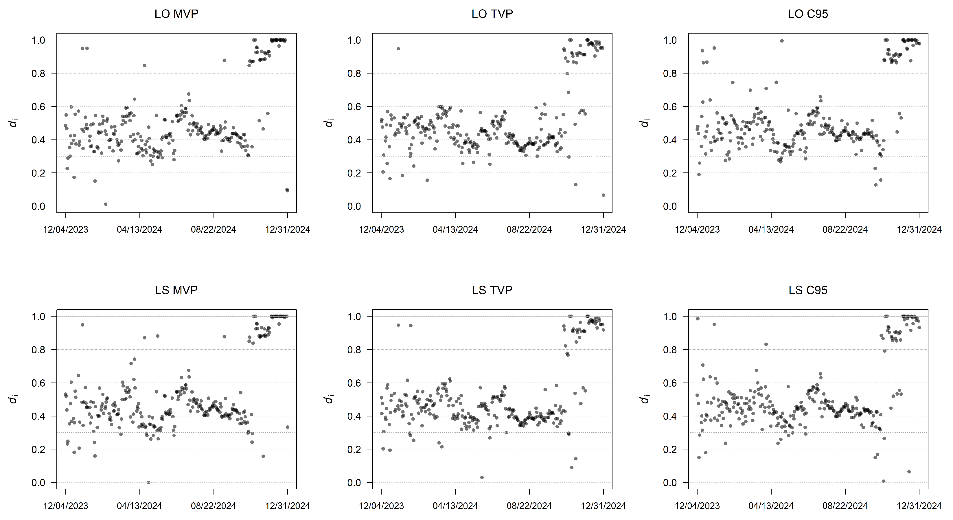
Values for $d_i$ lie in the range [0.3389, 0.4138], indicating persistence in the conditional variance. To examine whether this persistence was stable through time, we estimated the ARMA(3,2)–FIGARCH(1,d,1) model using rolling windows of length 252 trading days. Figure 7 reports the rolling window estimates for $d_i$ for the same six optimized portfolios. The rolling estimates suggest a transition toward stronger conditional-variance persistence near the end of the study period. With exceptions, the estimates tend to concentrate in the range $d_i\in [0.3,0.6]$ prior to the latter part of October 2024. During the end of October, there is a transition period, after which values of $d_i$ concentrate in the range [0.8, 1.0].

7. Regression on a Market Index

We estimated two single-factor regressions for the optimized portfolio strategies. Both are capital asset pricing models (CAPMs) (Lintner, 1965; Mossin, 1966; Sharpe, 1964); the first uses the BHP as an endogenous market index,

$$R_{i,t}-r_{f,t}={\alpha }_i+{\beta }_i\left(R_t^{\mathrm{BHP}}-r_{f,t}\right)+{\epsilon }_{i,t},$$

(5)

while the second

$$R_{i,t}-r_{f,t}={\alpha }_i+{\beta }_i\left(R_t^{\mathrm{DJIA}}-r_{f,t}\right)+{\epsilon }_{i,t},$$

(6)

uses the DJIA as an exogenous market index. In (5) and (6), $R_{i,t}$ is the return on strategy-optimized portfolio i, $R_t^{\mathrm{market}}$ is the market index return, and $r_{f,t}$ is the risk-free rate. $R_{i,t}-r_{f,t}$ and $R_t^{\mathrm{market}}-r_{f,t}$ are referred to as excess returns. Under CAPM, ${\beta }_i$ measures exposure to systematic market risk, ${\alpha }_i$ measures abnormal excess return relative to the market, and the residual ${\epsilon }_{i,t}$ is the idiosyncratic component of i. The residual can be standardized as $z_{i,t}={\epsilon }_{i,t}/{\sigma }_i$, where ${\sigma }_i^2$ (assumed time-independent) is the variance of ${\epsilon }_{i,t}$.

All regressions in this section were estimated using Huber $M-$estimation (Huber, 1981; Maronna et al., 2019) implemented in the MATLAB R2025a function robustfit. The pseudo-$R^2$ reported in the tables is the squared correlation between observed and fitted excess returns. RMSE is the root mean squared value of the error ${ϵ}_{i,t}$. Each regression used the 529 optimized returns computed for the study period.

Table 4. Parameter and goodness-of-fit estimates for the CAPM (5). The portfolios have been ordered in terms of increasing value of $\beta$.

Portfolio	$\mathit{\alpha }$ (×10−5)	SEα (×10−5)	${\mathit{p}}_{\mathit{\alpha }}$	$\mathit{\beta }$	SEβ (×10−3)	${\mathit{p}}_{\mathit{\beta }}$	Pseudo R2	RMSE (×10−3)
LS C99	−2.85	2.78	0.3065	0.967	3.150	****	0.9923	0.751
LO C99	−2.65	2.73	0.3309	0.967	3.085	****	0.9923	0.749
LO C95	−1.46	2.75	0.5968	0.968	3.112	****	0.9927	0.728
LO MVP	−4.74	2.85	0.0970	0.969	3.227	****	0.9911	0.805
LS MVP	−4.74	2.85	0.0970	0.969	3.227	****	0.9911	0.805
LS C95	−1.33	2.80	0.6352	0.969	3.172	****	0.9924	0.749
LS TVP	2.21	1.96	0.2621	0.998	2.223	****	0.9961	0.558
LS TC95	2.16	1.97	0.2734	0.998	2.226	****	0.9960	0.560
LS TC99	2.17	1.97	0.2703	0.998	2.227	****	0.9960	0.560
LO TVP	2.29	1.96	0.2426	1.000	2.219	****	0.9962	0.553
LO TC95	2.30	1.96	0.2420	1.000	2.221	****	0.9961	0.554
LO TC99	2.29	1.97	0.2448	1.000	2.224	****	0.9961	0.554

${\mathrm{SE}}_q$ denotes the standard error while $p_q$ denotes the p-value computed for parameter q. **** indicates a p-value less than ${10}^{-4}$.

reports the CAPM estimates obtained for the endogenous market index. The optimization strategies, listed in terms of the increasing value of the fitted values for $\beta$, cleanly separate into minimum-risk and tangent portfolios. This minimum risk versus tangent separation is seen in the fitted values of $\alpha$ (negative versus positive), ${\mathrm{SE}}_{\alpha }$ and ${\mathrm{SE}}_{\beta }$ (larger versus smaller values), $\beta$ ([0.966, 0.969] versus [0.998, 1.000]), pseudo-$R^2$ ([0.9911, 0.9927] versus [0.9960, 0.9962]), and RMSE (larger versus smaller values). For each numerical measure presented in Table 4, the variation in value for the tangent portfolios is much less than the variation in value for the minimum-risk portfolios. As expected for regression against an endogenous market index, the values of $\beta$ and pseudo-$R^2$ are very high. The positive values for $\alpha$ correlate well with the excess price values (relative to BHP) seen in the tangent portfolios of Figure 3. The fact that the p-values for $\alpha$ are not significant may reflect the difficulty in measuring the small values of $\alpha$. However, we judge the sign consistency in $\alpha$ between minimum-risk and tangent portfolios to be significant.

Table 5. Parameter and goodness-of-fit estimates for the CAPM (6). The BHP has been included as one of the portfolios regressed against DJIA. The portfolios have been ordered in terms of increasing value of $\beta$.

Portfolio	$\mathit{\alpha }$ (×10−5)	SEα (×10−5)	${\mathit{p}}_{\mathit{\alpha }}$	$\mathit{\beta }$	SEβ (×10−2)	${\mathit{p}}_{\mathit{\beta }}$	Pseudo R2	RMSE (×10−3)
LO MVP	−58.93	26.33	0.0256	0.763	3.67	****	0.4107	6.537
LS MVP	−58.93	26.33	0.0256	0.763	3.67	****	0.4107	6.537
LO C99	−57.66	26.14	0.0278	0.766	3.64	****	0.4141	6.512
LS C99	−57.35	26.08	0.0283	0.766	3.63	****	0.4138	6.514
LO C95	−58.18	26.00	0.0256	0.770	3.62	****	0.4148	6.522
LS C95	−58.45	25.92	0.0245	0.771	3.61	****	0.4152	6.525
BHP	−57.62	26.68	0.0312	0.809	3.72	****	0.4241	6.712
LS TVP	−55.06	26.66	0.0394	0.820	3.71	****	0.4258	6.722
LS TC95	−55.09	26.65	0.0392	0.820	3.71	****	0.4256	6.723
LS TC99	−55.11	26.66	0.0392	0.820	3.71	****	0.4256	6.724
LO TVP	−55.23	26.51	0.0377	0.824	3.69	****	0.4271	6.736
LO TC95	−55.22	26.53	0.0379	0.824	3.69	****	0.4270	6.737
LO TC99	−55.27	26.52	0.0376	0.824	3.69	****	0.4269	6.738

${\mathrm{SE}}_q$ denotes the standard error while $p_q$ denotes the p-value computed for parameter q. **** indicates p-value less than ${10}^{-4}$.

provides the CAPM estimates for the exogenous model (6). Optimization strategies are listed in the order of increasing value of $\beta$, which produces a reordering of the minimum-risk portfolios compared to that in Table 4. The clean separation between the minimum-risk and tangent portfolios is still seen in all measures, with the BHP “grouping with” the tangent portfolios. Compared to the tangent portfolios (and BHP), the minimum-risk values of all measures in Table 5 are smaller: $\alpha$ ([$-58.93,-57.35$] versus [$-57.62,-55.06$]); ${\mathrm{SE}}_{\alpha }$ ([25.92, 26.33] versus [26.51, 26.68]); $p_{\alpha }$ ([0.0245, 0.0283] versus [0.0312, 0.0394]); $\beta$ ([0.763, 0.771] versus [0.809, 0.824]); ${\mathrm{SE}}_{\beta }$ ([3.61, 3.67] versus [3.69, 3.72]); pseudo-$R^2$ ([0.4107, 0.4152] versus [0.4241, 0.4271]); and RMSE ([6.512, 6.537] versus [6.712, 6.738]). If the BHP values are excluded, the variation in each measured value for the tangent portfolios is less than the variation in value for the minimum-risk portfolios. In contrast to the results for the endogenous regression, the values of $\alpha$ computed for the exogenous fit are significant at the 5% level for the $p_{\alpha }$ values. As expected for regression against an exogenous market index, the values of $\beta$ and pseudo-$R^2$ are smaller than those found in the endogenous regression. The $R^2$ values of ∼40% correlate with the larger values of RMSE obtained for the exogenous fit compared with the endogenous fit.

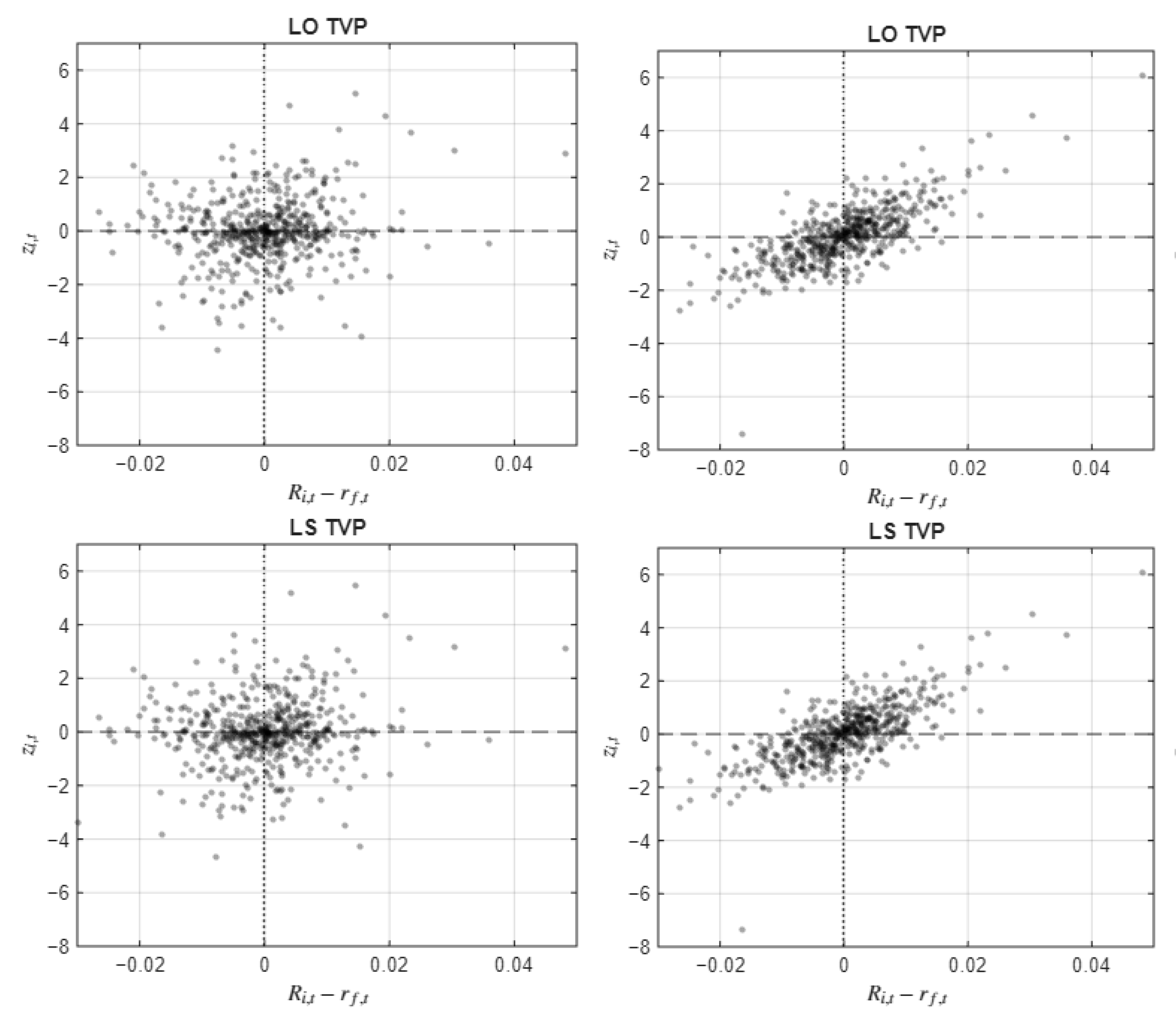
Figure 8 shows the standardized residuals $z_{i,t}$ plotted against the excess returns $R_{i,t}-r_{f,t}$ computed from the fits (5) and (6) for two of the strategy-optimized portfolios.

Table 6. Standard deviations of the excess returns and of the residuals and Pearson correlation coefficients from the CAPM fits for the strategy-optimized portfolios.

Portfolio	${\mathit{\sigma }}_{{\mathit{R}}_{\mathit{i},\mathit{t}}-{\mathit{r}}_{\mathit{f},\mathit{t}}}$	${\mathit{\sigma }}_{{\mathit{z}}_{\mathit{i},\mathit{t}}}$		${\mathit{\rho }}_{\mathit{z},\mathit{R}}$
$\mathit{i}$	(×10−3)	BHP	DJIA	BHP	DJIA
LO MVP	8.521	1.2293	1.0812	−0.0093	0.7654
LO C95	8.531	1.1531	1.0925	−0.0008	0.7613
LO C99	8.512	1.1951	1.0848	−0.0045	0.7627
LO TVP	8.904	1.2282	1.1066	0.1418	0.7469
LO TC95	8.905	1.2292	1.1059	0.1423	0.7469
LO TC99	8.905	1.2280	1.1066	0.1429	0.7469
LS MVP	8.521	1.2293	1.0812	−0.0093	0.7654
LS C95	8.537	1.1632	1.0963	−0.0022	0.7609
LS C99	8.513	1.1741	1.0877	0.0001	0.7629
LS TVP	8.876	1.2368	1.0982	0.1272	0.7479
LS TC95	8.876	1.2400	1.0987	0.1260	0.7479
LS TC99	8.876	1.2392	1.0985	0.1267	0.7480

provides the standard deviations ${\sigma }_{R_{i,t}-r_{f,t}}$ and ${\sigma }_{z_{i,t}}$ of the excess portfolio returns and residuals, respectively, and the Pearson correlation coefficients ${\rho }_{z,R}$ between $z_{i,t}$ and $R_{i,t}-r_{f,t}$ for the CAPM fits for the strategy-optimized portfolios. For the fit to the endogenous benchmark, the bivariate $(z_{i,t},R_{i,t}-r_{f,t})$ distribution appears uncorrelated for the minimum-risk portfolios and weakly positively correlated for the tangent portfolios. For the fit to the exogenous benchmark, the bivariate distribution is positively correlated, with a correlation coefficient just below 0.748 for the tangent portfolios and just above 0.760 for the minimum-variance portfolios.

8. Option Pricing Under NDIG Subordinated Dynamics

The NDIG subordinated price process introduced by Shirvani et al. (2024) defines the log-price dynamics $X\left(t\right)$ by

$$\begin{array}{cc}\hfill S_t& =e^{X\left(t\right)},t\in [0,\tau ],\hfill \\ \hfill X\left(t\right)& =X\left(0\right)+\mu t+\gamma U\left(t\right)+\rho T\left(U\right(t\left)\right)+\sigma B\left(T\right(U\left(t\right)\left)\right),\hfill \end{array}$$

(7)

where $B\left(t\right)$ is a standard Brownian motion, and $U\left(t\right)$ and $T\left(t\right)$ are Lévy subordinators. The Brownian motion produces the drift parameter $\mu$ and volatility $\sigma$. The subordinator $T\left(t\right)$ is modeled as inverse Gaussian (IG), $T\left(1\right)\sim \mathrm{IG}({\lambda }_T,{\mu }_T)$, having the probability density

$$f_{T\left(1\right)}\left(x\right)=\sqrt{{\displaystyle \frac{{\lambda }_T}{2\pi x^3}}}\exp \left(-{\displaystyle \frac{{\lambda }_T{(x-{\mu }_T)}^2}{2{\mu }_T^{2}x}}\right),{\lambda }_T>0,{\mu }_T>0,x\ge 0.$$

(8)

The subordinator $U\left(t\right)$ is also modeled as IG, $U\left(1\right)\sim \mathrm{IG}({\lambda }_U,{\mu }_U)$. The subordinators induce the additional drift terms with parameters $\gamma$ and $\rho$. Following Lindquist et al. (2022), to ensure unique values for $\gamma$ and $\rho$, we can assume ${\mu }_T={\mu }_U=1$. Using $U\left(t\right)$ to model stochastic time changes in the return process, we can reasonably assume $\gamma =0$, leaving five NDIG parameters in the model. The resultant model allows for skewness, kurtosis, and heavy tails in the stochastic return process. The parameters can be determined by matching to the first four centered moments and empirical characteristic function determined from a historical return sample (Lindquist et al., 2022).

Prices of European options were determined based on an optimized portfolio as the underlying risky asset. We report price surfaces for the LO C99-optimized portfolio. Specifically, we report options computed for the end date, $t=$ 31 December 2024, of the study period.

Table 7. NDIG parameters computed from the LO C99 portfolio log-returns.

$\mathit{\mu }$	$\mathit{\rho }$	$\mathit{\sigma }$	${\mathit{\lambda }}_{\mathit{T}}$	${\mathit{\lambda }}_{\mathit{U}}$
$-3.76\times {10}^{-4}$	$3.22\times {10}^{-4}$	$8.61\times {10}^{-3}$	$1.08$	$1.51$

presents the NDIG parameters estimated using the LO C99 portfolio log-returns over the study period.

To price the options, we followed the implementation of Lindquist et al. (2022, Chapter 12), which used the mean-correction martingale construction (Yao et al., 2016). Under the equivalent martingale measure $\mathbb{Q}$, the risk-neutral price process is

$$S_t^{\left(\mathrm{Q}\right)}=S_0\exp \left\{\left(r_f-K_{X_1}(1;\theta )\right)t+X_t\right\},$$

(9)

where $r_f$ is the (assumed time-independent) risk-free rate, $K_{X_1}(1;\theta )$ is the cumulant-generating function of the one-period log-return increment $X_1$, and $\theta =\{\mu ,\rho ,\sigma ,{\lambda }_T,{\lambda }_U\}$ is the parameter set upon which $K_{X_1}$ depends. This adjustment ensures that the discounted price process $e^{-r_{f}t}{S}_t^{\left(\mathbb{Q}\right)}$ is a martingale under $\mathbb{Q}$. The corresponding characteristic function of the log price is

$${\phi }_{\log S_t^{\left(\mathbb{Q}\right)}}(v;\theta )=S_0^{iv}\exp \left(\left[iv\{r_f-K_{X_1}(1;\theta )\}+{\psi }_{X_1}(v;\theta )\right]t\right),$$

(10)

where ${\psi }_{X_1}(v;\theta )$ is the characteristic exponent of $X_1$.

Call prices were computed using the Fourier transform method of Carr and Madan (1999),

$$C_{\mathrm{NDIG}}(S_t,\tau ,K,r_f;\theta )={\displaystyle \frac{e^{-r_f\tau -ak}}{\pi }}{\int }_0^{v_{\max }}{e}^{-ivk}{\displaystyle \frac{{\phi }_{\log S_{t+\tau }^{\left(\mathbb{Q}\right)}}\left(v-i(a+1);\theta \right)}{a^2+a-v^2+i(2a+1)v}}dv,$$

(11)

where $\tau =T-t$, T is the maturity time; $k=\log K$; $a>0$ is the Carr–Madan damping parameter, and $v_{\max }$ truncates the (infinite) upper limit of the Fourier integral. Put prices were obtained from put–call parity.

The damping parameter controls the exponential damping of the transformed call payoff. If a is too small, the computed option prices will violate the respective no-arbitrage upper bound. If a is too large, the computed option prices will violate the respective lower bound. The choice of a was adjusted until all computed option prices remained inside the no-arbitrage bounds

$$\begin{array}{cc}\hfill \max \{S_t-K{e}^{-r_f\tau },0\}& \le C_{\mathrm{NDIG}}(S_t,\tau ,K,r_f;\theta )\le S_t,\hfill \\ \hfill \max \{K{e}^{-r_f\tau }-S_t,0\}& \le P_{\mathrm{NDIG}}(S_t,\tau ,K,r_f;\theta )\le K{e}^{-r_f\tau }.\hfill \end{array}$$

(12)

(It is unnecessary to check both call and put option bounds. Under put–call parity, it is sufficient to ensure that the call option bounds are respected.)

The Fourier integral in (11) was evaluated on the finite interval $[0,v_{\max }]$. The computation of (11) as an FFT on a grid with N equally spaced values of v requires the discretizations $v_i=i\Delta v$ and $k_i=k_{\min }+i\Delta k$, $i=0,\dots ,N-1$, where

$$\Delta v={\displaystyle \frac{v_{\max }}{N-1}},\Delta k={\displaystyle \frac{2\pi }{N\Delta v}}.$$

(13)

The value of $v_{\max }$ must be large enough to produce a satisfactory truncation error, while the strike values $K_i=\exp k_i$ must cover an appropriate range of values.

Table 8. Additional parameter values used in the NDIG option-pricing computation for the LO C99-optimized portfolio.

${\mathit{S}}_{\mathit{t}}$	${\mathit{r}}_{\mathit{f}}$	a	N	${\mathit{v}}_{\mathbf{max}}$	Quadrature Rule
$97.18$	$1.107\times {10}^{-4}$	$1.25$	1024	595	Trapezoid

The value of $r_f$ was determined using the risk-free rate for 31 December 2024.

summarizes the numerical settings used in computing option prices for the date $t=$ 31 December 2024. Prices were computed for maturity times of $T=1,\dots ,200$ trading days and moneyness values $M=K/S_t\in [0.70,1.30]$.

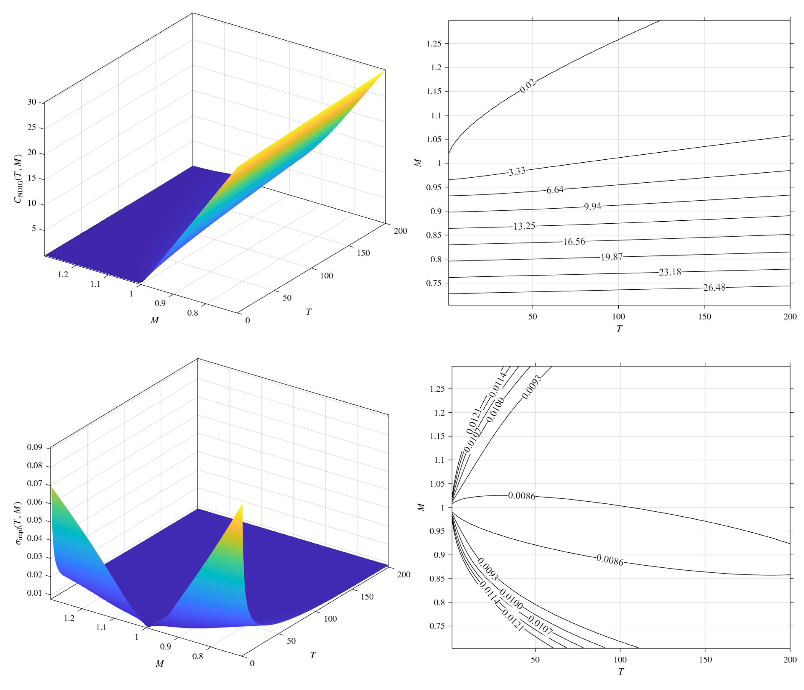
Figure 9 presents the computed NDIG call prices for options written on the LO C99-optimized portfolio. Prices are plotted as functions of maturity T and moneyness M. Also plotted are the projections of price contours onto the $T,M$ plane. Implied volatilities for empirical option data are frequently computed using the Black–Scholes formula. Considering the call prices $C_{\mathrm{NDIG}}(T,K)$ to be empirical data, we computed implied volatilities via

$${\sigma }_{\mathrm{impl}}(T,M)=\underset{\sigma >0}{\arg \min }{\left[{\displaystyle \frac{C_{\mathrm{BS}}(S_t,T,K,r_f,\sigma )-C_{\mathrm{NDIG}}(T,K)}{C_{\mathrm{NDIG}}(T,K)}}\right]}^2,$$

(14)

where $C_{\mathrm{BS}}(S_t,T,K,r_f,\sigma )$ denotes the Black–Scholes call price formula. The resultant surface ${\sigma }_{\mathrm{impl}}(T,M)$ and its contours projected on the $T,M$ plane are presented in Figure 9. A strong volatility smile is evident.

The contours labeled 0.0086 approximate the volatility value (0.0085) of the LO C99 portfolio as measured over the study period (Table 1). Generally over the $(T,M)$ plane, the computed implied volatility exceeded the study-period-measured volatility.

9. Discussion

We examined the performance of select strategy-optimized portfolios, each comprised of a universe of 30 real estate securities, over the period 4 January 2021 to 31 December 2024 using a variety of tail-sensitive techniques and measures (overlays). The tail-sensitive CVaR optimization performed better than mean-variance for minimum-risk portfolios; for tangent portfolios, there appeared to be no appreciable difference between CVaR and mean–variance optimization.

The analysis of the tail behavior of the optimized return distributions indicates control on overall skewness, kurtosis, and tail heaviness. The optimized portfolio return distributions had excess kurtosis restricted to the range [2.45, 2.65] and positive skewness in the range [0.225, 0.272]. Tail index estimates were slightly higher for the lower (loss) tail than for the upper (gain) tail of the return distribution.

Minimum-risk portfolios had lower Sharpe, Sortino, and information ratios, volatility, and maximum drawdown than tangent portfolios. In contrast, minimum-risk portfolios tended to have slightly higher Rachev ratios. The only noticeable difference between mean–variance and CVaR optimizations occurred in the Sharpe, Sortino, and information ratios for minimum-risk portfolios, where the ratio values were more negative for mean–variance than for CVaR optimization. As expected, minimum-risk portfolios had smaller values of ${\mathrm{VaR}}_{1-\alpha }$ and ${\mathrm{CVaR}}_{1-\alpha }$, $\alpha \in \{0.05,0.01\}$ than tangent portfolios. There was a negligible difference between mean–variance and CVaR optimization in these measures.

Tests using an ARFIMA-GARCH model with normally distributed innovations resulted in a finding of no significant evidence for long-range dependence in the conditional mean of the strategy-optimized portfolios. Tests using ARMA-FIGARCH with normally distributed innovations did produce a finding of moderate (fractional integration parameter $d\in [0.33,0.41]$) persistence in the conditional volatility. Performing the same analysis using moving windows revealed a transition period from moderate to higher persistence occurring during the later part of October 2024.

CAPM regression against the endogenous market index BHP produced a clean separation between minimum-risk and tangent portfolios, with minimum-risk portfolios having negative “alpha”, smaller “beta” (although all values of $\beta$ exceeded 96%), and larger RMSE. Variation in each respective value for the tangent portfolios was smaller than for minimum-risk portfolios. For the tangent portfolios, there was a suggestion of a consistent difference in values of $\alpha$ and $\beta$ between the long–short and long-only strategies. CAPM regression against the exogenous market index DJIA resulted in smaller values of $R^2$ (∼41%) and $\beta$ (∼0.8). Values of $\alpha$ were smaller and negative for all strategy optimizations. The clean separation between minimum-risk and tangent portfolios remained, with minimum-risk portfolios having $\alpha$ values that were slightly more negative and $\beta$ values that were slightly smaller. The suggestion of consistent difference in values of $\alpha$ and $\beta$ between the long–short and long-only strategies for the tangent portfolios remained. The CAPM residuals $z_{i,t}$ were either uncorrelated or only very weakly correlated with the excess return $R_{i,t}-r_{f,t}$ for the fit to the endogenous benchmark, but were positively correlated for the fit to the exogenous benchmark.

Option prices computed under the doubly subordinated NDIG model for the LO C99 strategy-optimized portfolio produced an implied volatility surface with a strong “smile” and implied volatilities that generally exceeded those computed for LO C99 over the study period. We recognize that this computation of an option price chain for a single date, for only one of the optimized portfolios, presents an extremely limited sample. Our goal has been to demonstrate the practical nature of performing portfolio optimization and derivative valuation within a common, tail-sensitive framework.

While we have pursued a fairly extensive downside-sensitive analysis of optimized portfolios based upon these 30 real estate securities, our results are clearly restricted to the 2021–2024 sample period, which does, however, include the post-pandemic recovery and the interest-rate tightening cycle. While an extension to a longer sample period covering additional market regimes would be of interest, our primary goal has been to demonstrate the benefits of a multi-layered approach to portfolio evaluation.