Article

Investigating the Relationship between Air Pollutants and Meteorological Parameters Using Satellite Data over Bangladesh

1
Laboratory of Atmospheric Physico-Chemistry, Anhui Institute of Optics and Fine Mechanics, Hefei Institutes of Physical Science, Chinese Academy of Sciences, Hefei 230031, China
2
Department of Electrical and Electronic Engineering, Pabna University of Science and Technology, Pabna 6600, Bangladesh
3
Department of Biosystems and Agricultural Engineering, Oklahoma State University, Stillwater, OK 74078, USA
*
Author to whom correspondence should be addressed.
Remote Sens. 2022, 14(12), 2757; https://doi.org/10.3390/rs14122757
Submission received: 22 April 2022 / Revised: 31 May 2022 / Accepted: 3 June 2022 / Published: 8 June 2022
(This article belongs to the Special Issue Stereoscopic Remote Sensing of Air Pollutants and Applications)

Abstract

:
Understanding of the relationship between air pollutants and meteorological parameters on the regional scale is a prerequisite for setting up air pollution prevention and control strategies; however, there is a lack of methodical investigations, particularly in the context of Bangladesh’s deficiency of information on air pollution. This study represents the first attempt to investigate the relationship between air pollutants (NO2, O3, SO2, and CO) and meteorological parameters over Bangladesh using satellite data (OMI and MOPITT) during the period from 2015 to 2020. Geographically weighted regression (GWR) modelling was utilized to assess the relationship between air pollutants and weather variables. The spatial representation and average values of geographically varying coefficients showed that the column densities of air pollutants were affected by the meteorological parameters. For example, NO2 was positively associated with temperature in most of the studied regions, with an average geographically varying coefficient value of 0.12 Dobson units (DU, 1 DU = 2.687 × 10¹⁶ molecules/cm2), indicating that NO2 concentrations increase by 0.12 DU/year with every unit increase in temperature. The sources of NO2 and SO2 in Dhaka were identified through emission inventory analysis, and transportation and industry emissions were the most significant influencing factors for NO2 and SO2, respectively. Temperature and pressure showed a higher degree of relationship with all four air pollutants compared with other parameters. The results and discussion presented in this study can be of benefit for policy makers in developing air pollution control strategies in Bangladesh.

1. Introduction

In recent decades, air pollution has become the prime concern of most nations in the world due to the intensification of human activities and adverse meteorological situations. Severe air pollution has caused negative health impacts and resulted economic losses [1,2]. Several studies have explored multiple human health issues caused by air pollution, such as cardiovascular and pulmonary ailments [3,4,5], diabetes and high blood pressure [6], premature deaths [7], mental health problem [8], etc. These findings were obtained based on several government and non-government organization data sets from in situ and satellite measurements. The capability of assessing the impact of air pollution on the regional to global scale is becoming more prominent due to the availability of satellite measurements of air pollutants [9].
Asian countries such as China, India, Pakistan, Nepal are facing severe air pollution due to the rapid urbanization and industrialization that have occurred over the past three decades. China was facing severe air pollution by 2013 [10,11,12] that was about five times higher than the safety level established by the WHO (World Health Organization). However, China has recovered from this negative situation by setting up strong policies and guidelines to fight air pollution. In previous studies [13,14] researchers were motivated to investigate the association between air pollution and other atmospheric components to set up the required policies with respect to spatial and temporal variations. Clean air policies (emissions control by different sectors, such as energy, top-down policy initiatives, and citizen engagement) employed by China during the period from 2014 to 2015 resulted in yearly average decreases of 4.9%, 12.0%, and 5.3% for NO2, SO2, and CO, respectively, and the primary determining factor was meteorological condition for more than 70% of cases in major Chinese cities [15]. Similarly, other countries are trying to improve their air quality, and the air quality of surrounding nations was partially improved as a result of the major improvement achieved in China. In this regard, Bangladesh is also affected by air pollution; mega cities such as Dhaka, Rajshahi, and Chittagong are seriously polluted with a variety of air pollutants [16,17], with pollution in the capital city, Dhaka [18,19]. However, information on air pollutants and their relationship with meteorological variables on the regional scale across the country is lacking.
The understanding of spatiotemporal characteristics of air pollutants over Bangladesh is very important for policy makers to set up pollution reduction guidelines. Along with anthropogenic emissions, adverse meteorological conditions, i.e., climate change phenomena, are highly responsible for air pollution [20,21,22,23]. The findings previous studies revealed the dependency of air pollution on different meteorological parameters over different cities, with temperature, pressure, and wind speed considered to be major affecting factors [24]. It is clear that the systematic understanding of the association between air pollutants and meteorological variables on the regional scale is a precondition for setting up air pollution prevention and control strategies. Although several potential studies have attempted to investigate the systematic relationship between air pollutants and meteorological variables [25,26,27], there is still a lack of methodical investigations at a meaningful regional scale, particularly in the context of Bangladesh, due to a scarcity of information on air pollution and its association with weather conditions on a national scale.
Some studies have evaluated the relationship between air pollutants and meteorological variables using sole regression and generalized additive models, although they did not take into account the spatial variability in this relationships [27,28,29]. Complex topological features, meteorological conditions, and anthropogenic emissions affect these relationships with considerable heterogeneity in the study region. On the other hand, geographically weighted regression (GWR) models investigate the non-stationary and scale- dependent characteristics of the association among dependent and independent variables [30], elucidating spatially varied relationships. Therefore, in the present study, we evaluated spatial relationships among metrological variables and air pollutants using coefficients from a GWR model. In the target study area, Bangladesh, it is difficult to obtain in situ measurements of air pollutants and meteorological parameters with optimal resolution for spatial analysis at a national scale. In this study, we used the monthly average data of four air pollutants (NO2, O3, SO2, and CO) from satellite data and seven meteorological parameters (temperature, pressure, specific humidity, wind speed, rainfall, solar radiation, and latent heat flux or evapotranspiration [31]) from GLDAS (Global Land Data Assimilation System) over Bangladesh from January 2015 to December 2020 to determine the spatiotemporal characteristics of air pollutants and meteorological parameters.
The main objectives of this study can be expressed as follows: (i) to observe the mean annual and seasonal distribution of air pollutants over Bangladesh; (ii) to investigate the trends in air pollutants and meteorological variables from 2015 to 2020 over the study region; and (iii) to investigate the spatial relationship between air pollutants and meteorological parameters at a pixel scale using a GWR model.

2. Materials and Methods
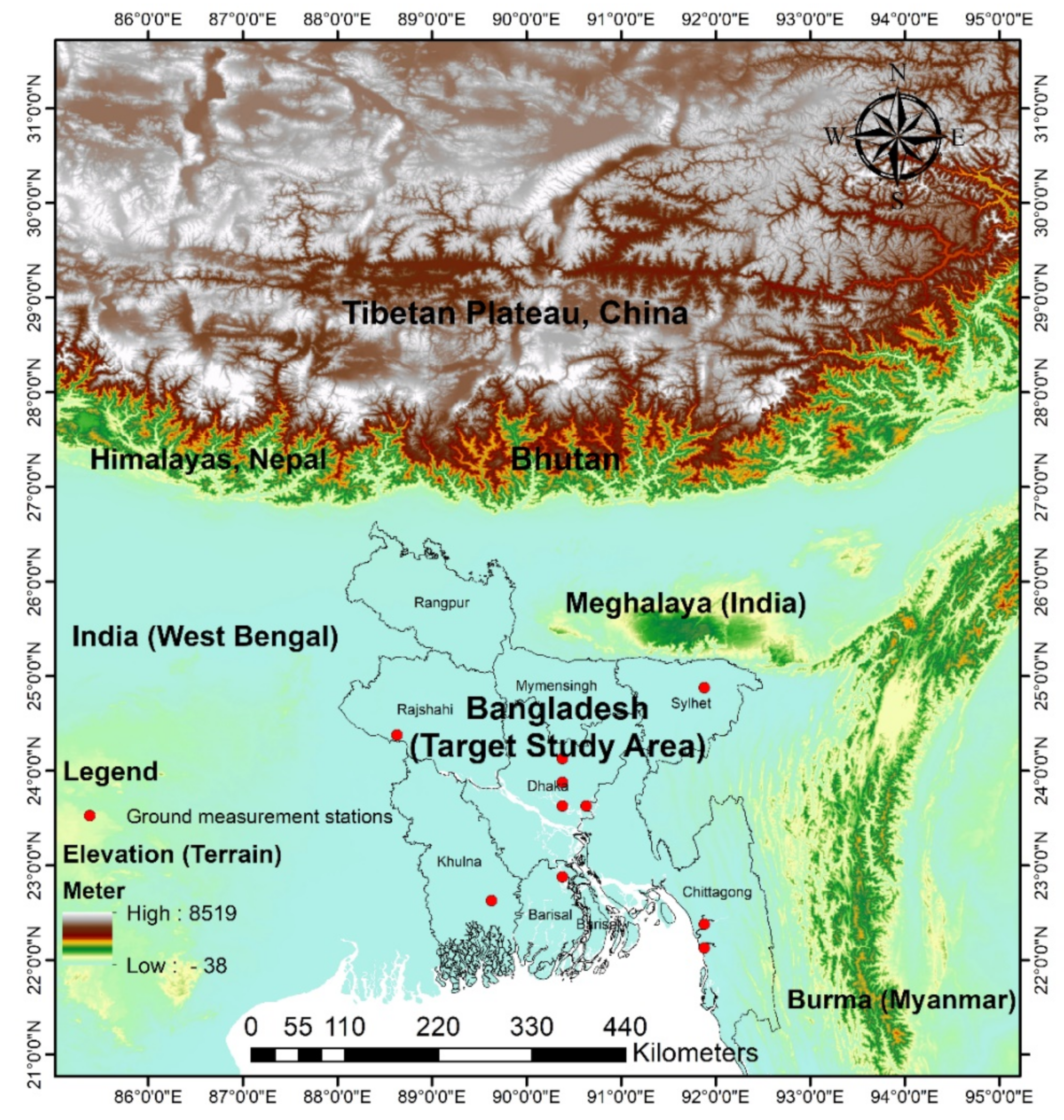
2.1. Study Area

The study area is Bangladesh, which lies between the latitudes of 20 ° N and 27 ° N and the longitudes of 88 ° E and 93 ° E, as shown in Figure 1. This country is located in the great delta of Ganges [32,33,34] of south Asia and is mostly surrounded by India, the Himalayas, the Tibetan Plateau, Myanmar (Burma), Bhutan, and the Bay of Bengal, with a total approximate land area of 147,570 km2. The land mass is of mostly plains, with average elevation of 10 m ASL (above sea level), with the maximum altitude in the north (105 m ASL) and a small hill system in the southeastern region of the country. Bangladesh has three distinguished seasons—summer (rainy season), autumn, and winter—with heat dominating in summer [35]. Bangladesh has a tropical monsoon climate (there is a practical lead/lag relationship between Indian continental monsoon and meteorological parameters [36]), which can be characterized by noticeable seasonal variation in humidity, temperature, and rainfall between summer (hot, humid, and rainy) from March to August, autumn (hot–warm) from September to November, and winter (dry) from December to February. Temperature ranges from 30 ° C to 40 ° C in summer and 10 ° C to 25 ° C in winter.

2.2. Data Description

As shown in Table 1, the satellite-based measurement data of four air pollutants (NO2, O3, SO2, and CO) were obtained from the OMI (Ozone Monitoring Instrument, Greenbelt, Maryland) of the Aura satellite [37,38,39] and MOPITT (Measurement of Pollution In The Troposphere) of the Terra satellite [40,41] from 2015 to 2020. Seven meteorological parameters were obtained from GLDAS (Global Land Data Assimilation System): temperature, pressure, specific humidity, wind speed, rainfall, solar radiation, and latent heat flux and evapotranspiration [42,43,44,45,46].
Surface-measured air pollutants were used in this study to compare the trend with the satellite-estimated data at some monitoring stations, as indicated in Figure 1. An AC32M chemiluminescence gas analyzer (TELEDYENE/API, San Diego, CA, USA, https://www.teledyne-api.com/applications/ambient-air-monitoring, (accessed on 20 November 2021)) was utilized to monitor the ground NO2, and an AF22M UV-fluorescence instrument (TELEDYENE/API, USA) was utilized to measure the ground SO2 in the CAMS (Continuous Air Monitoring Stations) project of the Ministry of Environment and Forests, Bangladesh (http://case.doe.gov.bd/, (accessed on 21 November 2021)). Only NO2 and SO2 measurements are reported here in order to observe the comparison between the satellite measurements (column densities) and ground measurements (instrument mixing ratios). Similar trends were found between these measurements, as shown in Figure 2, indicating the validity of the data in our study area.

2.3. Methods

The time-series raster data of the desired parameters were transformed into values using the ‘extract values to points’ technique in GIS (Geographic Information System), as well as the interpolation technique (Kriging) for spatial representations. The average seasonal variations of the air pollutants were observed using the monthly data as per the defined three practical seasons in Bangladesh: March-August (summer), September-November (autumn), and December-February (winter). The curve-fitting technique of GIS was applied to perform trend analysis of both the air pollutant and meteorological parameters over the country, where the value of the slope indicated the nature of the trend, i.e., increasing or decreasing trend with significance (p values).
A GWR model was extensively used in this study to investigate the relationship between air pollutants and meteorological parameters in Bangladesh on a national scale. GWR modelling is a type of regression modelling with geographically varying parameters (temperature, humidity, pressure, solar radiation, air pollutants, etc.), which is different from conventional regression modelling in that it was developed to obtain higher performance in geographical analysis. In general, the GWR model [47,48,49] can be expressed by the following equation.
D V i = k β k X i Y i I V k , i + ε i ,
where D V i is the dependent variable at location 𝑖; X i Y i is the X-Y coordinate of the 𝑖th location; β k X i Y i is the varying conditional coefficient at the kth and respective X-Y location with first coefficient by setting I V 0 , i = 1; β 0 X i Y i is defined as the geographically varying intercept term; I V k , i is the independent variable at the kth and respective X-Y location; and ε i is the Gaussain error at the x-y coordinate of the 𝑖th location.
In the case of our study, the GWR model can be described as:
A P i = β 0 X i , Y i + β 1 X i , Y i T i + β 2 X i , Y i P i + β 3 X i , Y i S H i + β 4 X i , Y i W S i + β 5 X i , Y i R f i + β 6 X i , Y i S R i + β 7 X i , Y i L E i + ε i ,
where A P i is the dependent air pollutants (NO2, O3, SO2, and CO); β 0 X i , Y i is the geographical intercept; β 1 to 7 X i , Y i are the geographically varying coefficients, which are different from the coefficients of conventional regression; and T, P, SH, WS, Rf, SR, and LE are the independent meteorological parameters (temperature, pressure, wind speed, rainfall, solar radiation, and latent heat flux, respectively) at the X-Y coordinate of the ith location.

3. Results

In this study, we presented the spatiotemporal characteristics of air pollutants from 2015 to 2020 with observations collected through OMI and MOPITT satellite data. Figure 3 represents the mean distribution of air pollutants from 2015 to 2020 over the target study region and its surroundings. A strong heterogeneity in NO2 concentration was observed in the study area, with the highest values (~7.91 × 10¹⁵ molecules/cm2) in the central part of Bangladesh (e.g., the capital city, Dhaka), as well as in the western surroundings (West Bengal, India). O3 concentration varied from 258 to 276 × 1018 molecules/cm2, with generally low values observed over Bangladesh, except the northernmost region, where its concentration was relatively higher. The SO2 distribution was generally random, with low concentrations observed in the central region of Bangladesh, whereas the western surroundings (India) had a relatively higher concentration. In contrast, the CO concentration was relatively higher over the whole country compared to the northern surroundings (Himalayas and Tibetan Plateau). These findings confirm that there is a significant heterogeneity in air pollutants across the country, particularly for NO2 and CO. Overall, the mean values of NO2, O3, SO2, and CO were 1.87 × 10¹⁵ molecules/cm2, 268.12 Dobson units (DU)~7.21 × 10¹⁸ molecules/cm2, 0.0945 DU~2.54 × 10¹⁵ molecules/cm2, and 2.75 × 10¹⁸ molecules/cm2, respectively.
Dobson units (DU) indicate the column density, whereas µg/m3, ppb (parts per billion in volume), or ppm (parts per million in volume) indicate concentrations. Therefore, we were not able to relate the DU and µg/m3, ppb, or ppm directly. Here, we can follow the following conversion steps [50,51,52]. For conversion purposes, 1 DU is equal to 2.69 × 1025 molecules/m3; to obtain the column density, it is necessary to integrate the total column over a height, which is 0.01 mm as per the 1 DU definition, i.e., 2.69 × 10²⁰ molecules/m2~2.69 × 1016 molecules/cm2. With respect to molecular weight, 1 DU is equal to 4.46 × 10⁻⁴ mol/m2, i.e., 2.14 × 10⁴ µg/m2 for ozone (O3); for other air pollutants (SO2, NO2, and CO) it is necessary to use the conversion factors listed in Table 2.

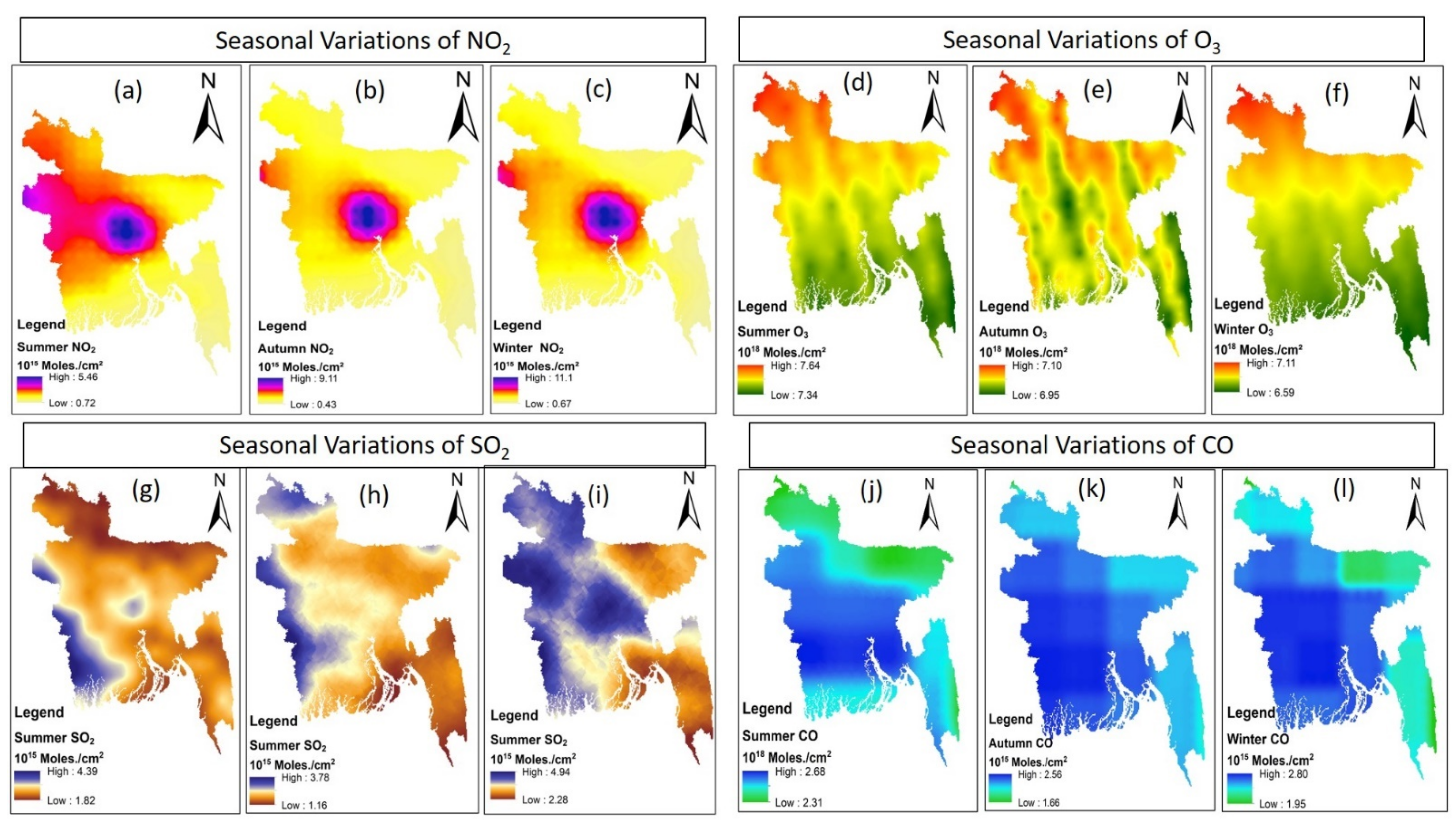
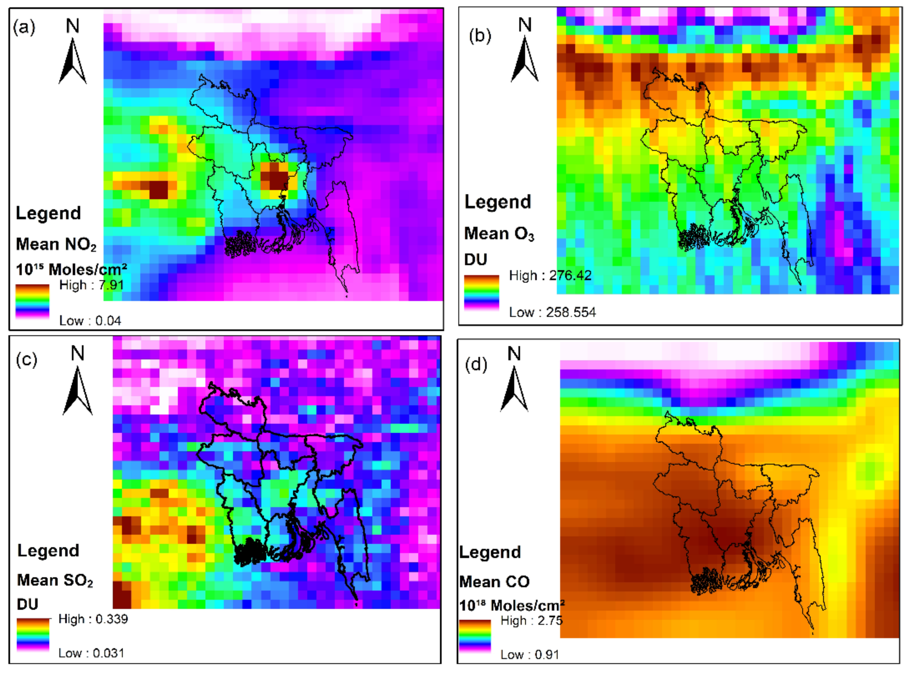
3.1. Average Seaonal Variation in Air Pollutants

Anthropogenic and climate variables significantly influence air pollutant emissions across seasons [53]. The average seasonal variations (2015–2020) of the four air pollutants are presented in Figure 4. NO2 concentration varies among all seasons, with the highest values observed in winter in contrast to summer and autumn seasons. Interestingly, NO2 concentration was relatively higher in the central part of the study region during all seasons, without any significant variations. The central region includes the capital city of Bangladesh, which is densely populated with the highest traffic flow [54].
Figure 4d–f illustrates the average seasonal distribution of O3 from 2015 to 2020 in the study region. The O3 concentration was higher in the northern region and, with lower values in the southern region during all seasons. However, in autumn, O3 spread from the northern region towards the central regions, with higher concentrations in the east. The O3 distribution in winter and summer seasons was similar, with slight differences. Overall, the distribution of O3 across the country did not differ significantly across seasons, and concentration remained constant throughout the year.
Relatively low concentrations of SO2 were distributed over the entire study region in summer and autumn. In contrast, its concentration was obviously hazardous in winter over the entire study area, especially the central regions, except for eastern coastal areas, where its concentration remained low during all seasons. Overall, SO2 levels varied significantly across seasons, with the variations being most visible in the central regions. There were slight variations in CO concentration in the east regions (Figure 4j–l).

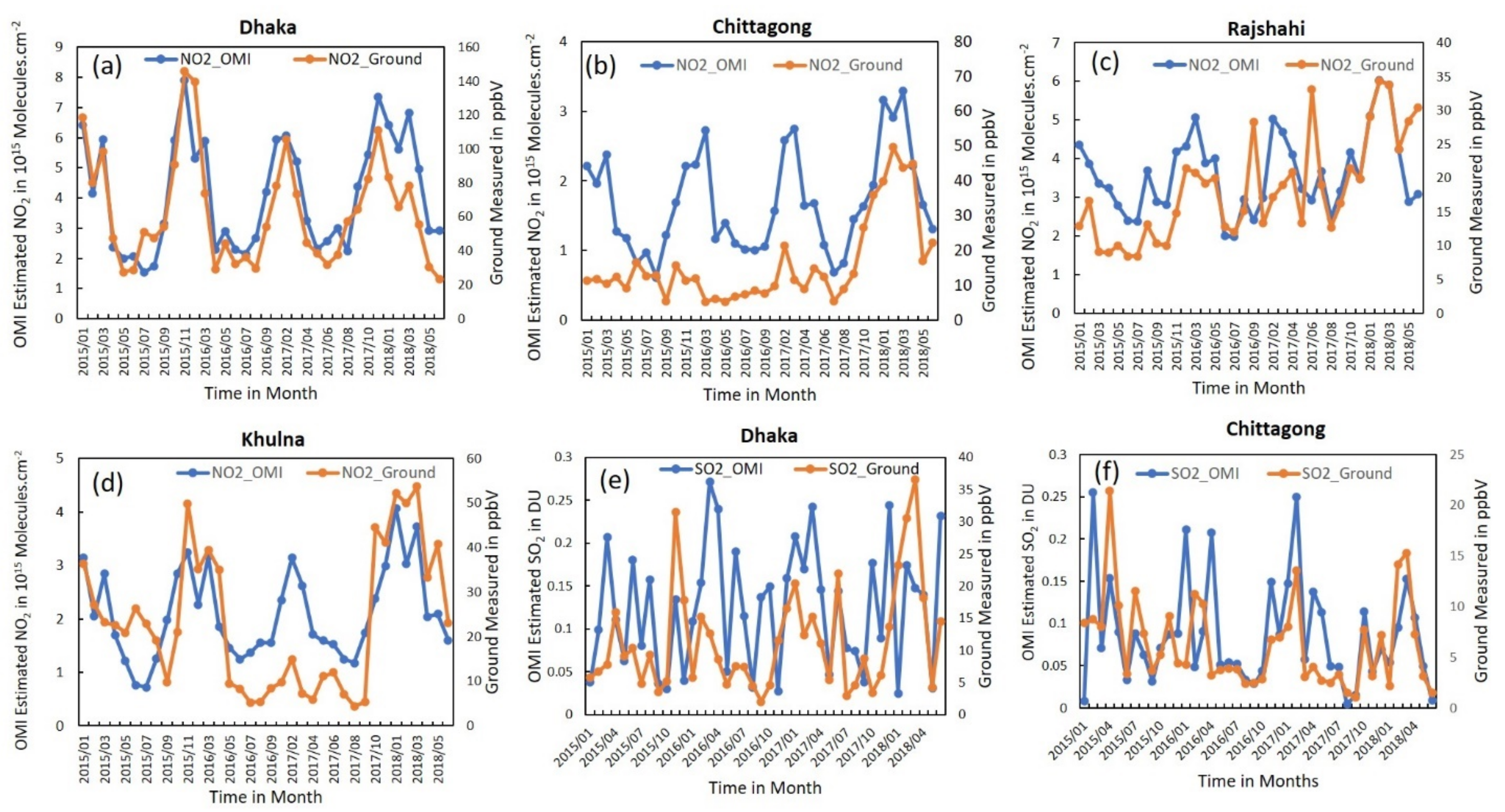
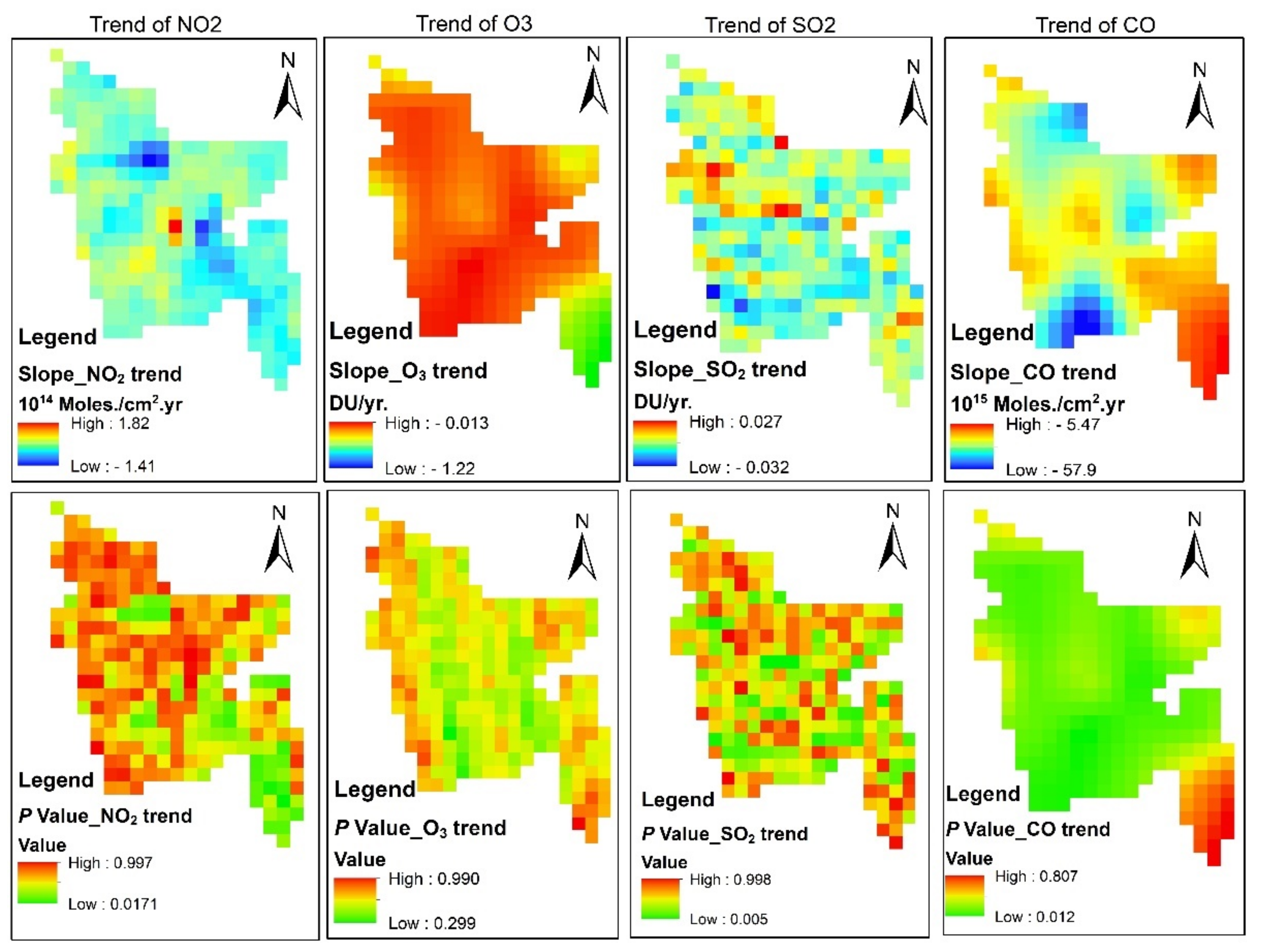
3.2. Trend Analysis of Air Pollutants

We performed a spatial trend analysis on average annual concentrations of air pollutants from 2015 to 2020, as presented in Figure 5. The changing trends for NO2 and CO were more heterogeneous, whereas the trends for O3 and SO2 were random in the study region. The most significant increasing trend for NO2 was 1.82 × 10¹⁴ molecules/cm2 per year (central area, i.e., Dhaka, with mean increasing rate of 9.7% as compared to the average of 6 years). This scenario might have been caused by the massive traffic flow and anthropogenic emissions associated with economic development [55]. In the case of SO2, the trend over the country was random, with an increasing value observed near Dhaka, and the highest value of 0.027 DU per year recorded in the western region, i.e., the increasing rate was 28.5% in the central and western regions of the country. In contrast, the observed trend for CO decreased over the whole country, with the lowest decreasing trend (−5.47 × 10¹⁵ molecules/cm2, i.e., −0.19%) corresponding to the central, southeastern, southwestern, and northeastern regions. The p values for CO were highly significant (<0.05) over the entire study region, whereas a mix trend was observed for NO2 and SO2.

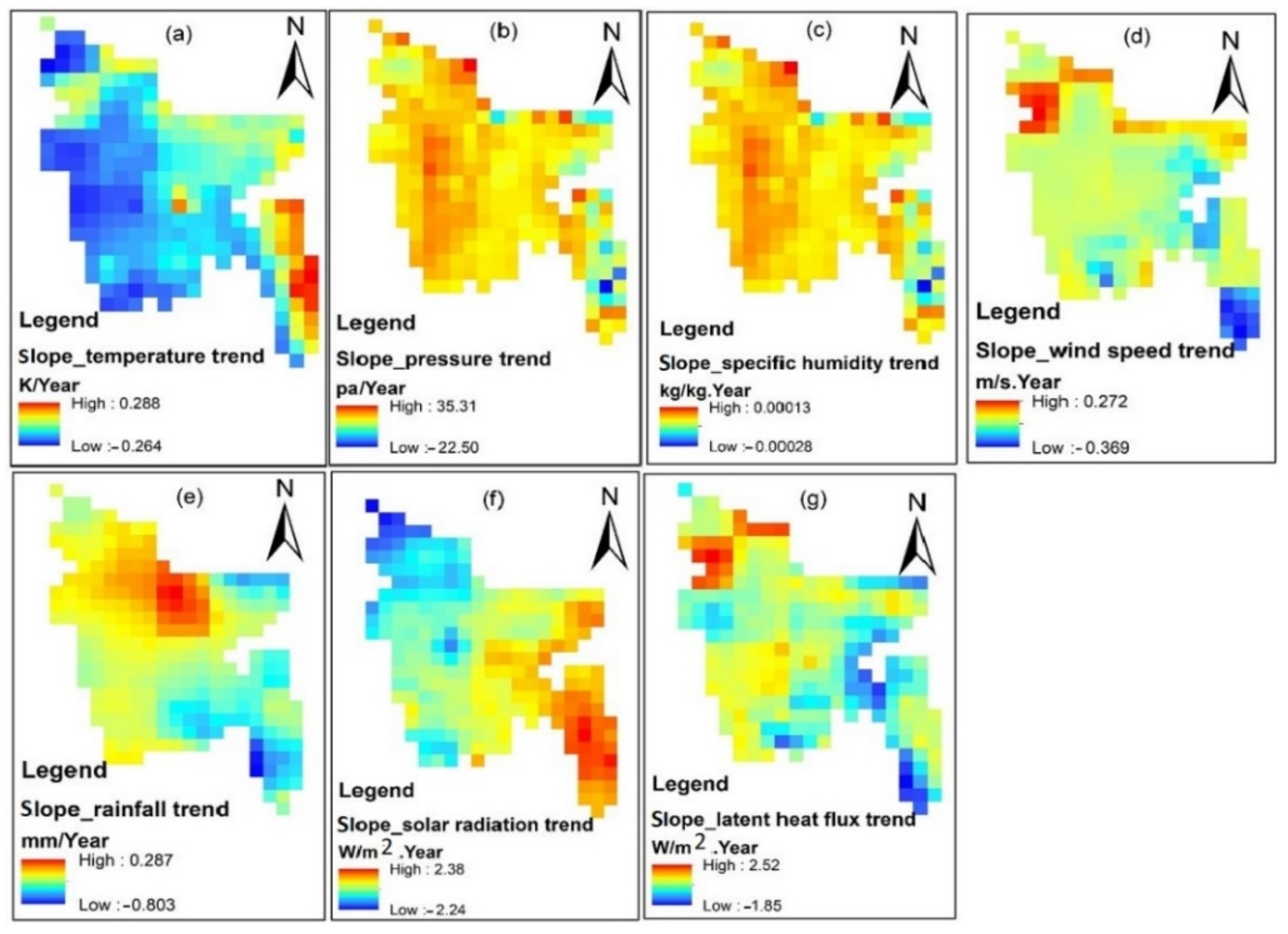
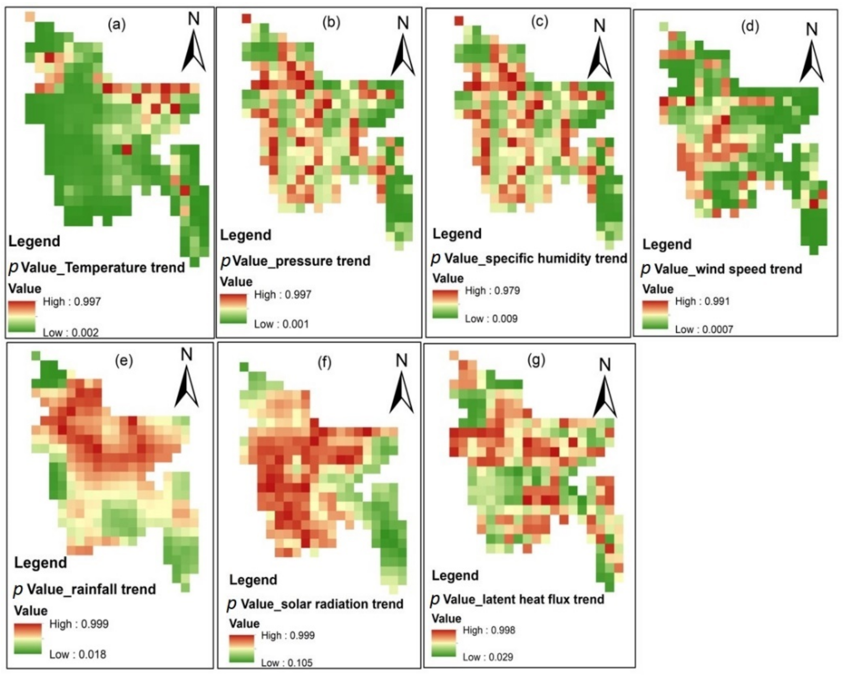
3.3. Trend Analysis of Meteorological Parameters

Figure 6 summarizes the spatial maps of trend analysis for seven meteorological parameters, and Figure 7 displays the corresponding p values. An increasing trend was more prominent in the case of specific humidity, pressure, wind speed, and latent heat flux across the study region. The pressure showed a mostly moderate to high increasing trend (35.31 pa/year) across the entire study region. Wind speed increased across the entire study region, but the trend was more pronounced in the northern areas, where it increased at a rate of 0.27 m/s per year. However, a slight decreasing trend was also observed along the south coastal areas. A random trend was observed for latent heat flux, similar to the trend for wind speed but with different values. The temperature trend seemed to slightly decrease (−0.264 K/year), especially in the western regions of the study area, with a slight increase (0.288 K/year) observed along the southeastern coastal regions. Rainfall and solar radiation presented opposite and heterogeneous trends, with an increase in rainfall observed in the northern regions (0.28 mm/year), which was associated with a decrease in solar radiation (−2.24 W/m2 per year). In contrast, the rainfall trend decreased by −0.82 mm/year, which was associated with an increasing (2.38 W/m2 per year) trend of solar radiations in the southeastern region. Figure 7 shows the respective p values for seven meteorological parameters over Bangladesh according to a spatial trend analysis. The decreasing trend in temperature was highly significant (p < 0.05) across the study region. In the case of pressure, specific humidity, and wind speed, the p value was randomly distributed (significant and non-significant), with the highest significant trend observed in the western regions. In the case of rainfall and solar radiation trend analysis, the p values were non-significant in most regions, and in the case of latent heat, the p value was randomly distributed and significant in the same area, where it presented as an increasing trend.

3.4. Relationship between Air Pollutants and Meteorological Parameters

The geographically varying coefficients obtained from the GWR model (the weight value was estimated for these coefficients) were used to investigate the relationship between air pollutants and meteorological parameters. Using output values of the GWR model, in this study, we performed a spatial distribution analysis of geographically varying coefficients using interpolation techniques to explain the relationship between pollutants and meteorological parameters over Bangladesh.

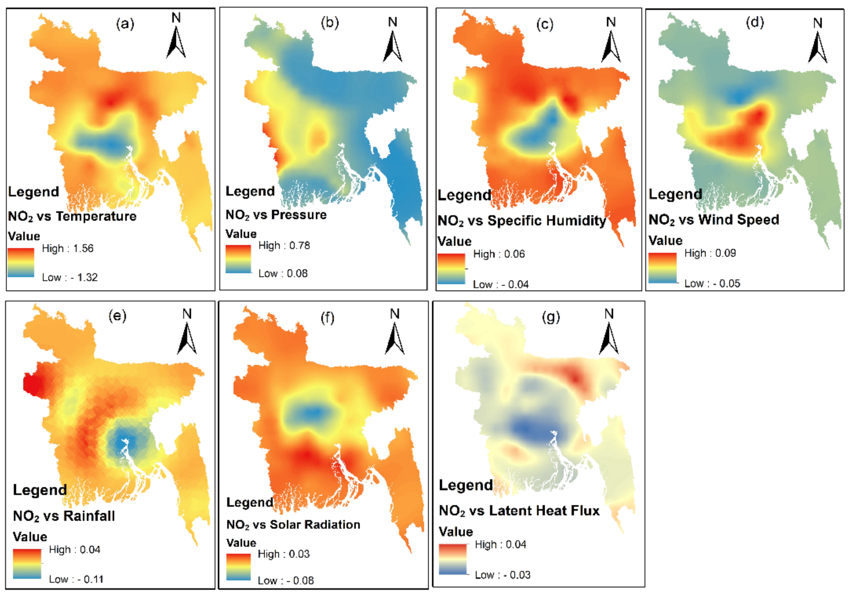
3.4.1. Spatial Relationship between NO2 and Meteorological Variables

The spatial characteristics of the geographically varying coefficients between NO2 and meteorological parameters are presented in Figure 8. Higher positive coefficient values indicate a greater contribution to increasing NO2 with per unit increase over the entire study period and vice-versa. For example, temperature coefficients were significantly positive across most study regions, ranging from 0 to 1.56 DU, indicating that the NO2 concentration was increased by a maximum of 1.56 DU~4.19 × 10¹⁶ molecules/cm2/year for every unit increase in temperature, while controlling the effects of other variables. However, temperature coefficients were negatively correlated across in the central–southern region. NO2, rainfall, specific humidity, and solar radiation all exhibited a pattern similar to that of temperature, with negative coefficient values in the central regions and higher positive values in the surrounding regions. NO2 and pressure showed positive associations all over the country, the with a maximum value of 0.78 DU and a minimum value of 0.08 DU. NO2 and latent heat flux showed a random pattern across the country, with negative associations with NO2 in the central region and its surroundings. Overall, comparison among all meteorological coefficients indicated that the temperature coefficient was highest (1.56), followed by pressure (0.78) and wind speed (0.09), indicating that these meteorological parameters contribute considerably to the changing trend of NO2 concentration across the study area. Similar findings have been reported in previous studies [27,56,57].

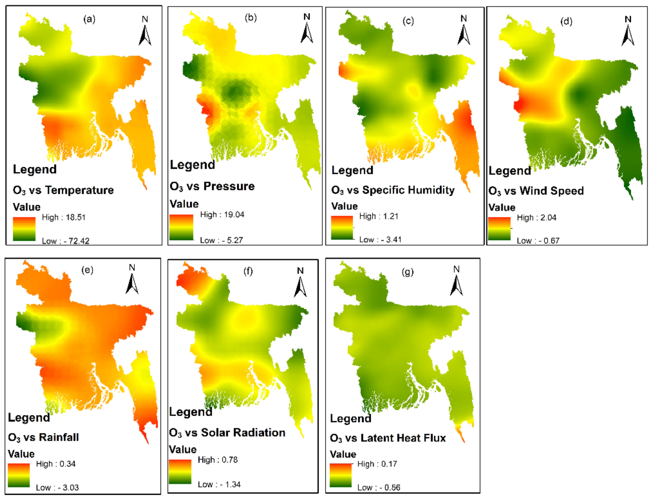
3.4.2. Spatial Relationship between O3 and Meteorological Variables

Figure 9 shows the spatially interpolated geographically varying coefficients representing the relationship between O3 and the meteorological parameters. The northeastern, southeastern, and southwestern parts of the country presented a positive association between O3 temperature, with a maximum increasing value of 18.51 DU, whereas the northwestern region presented a negative relationship, with a maximum decreasing value of −72.42 DU (Figure 9a).The relationship between O3 and pressure was heterogeneous, with negative coefficient values observed in the central regions, whereas higher positive values were observed in the southwestern region, with a value of 19.04 DU (Figure 9b). A relationship between O3 and specific humidity was observed, with negative distribution (maximum value of −3.41 DU) across most of the study region, which is consistent with the resulted of previous studies [56], exception in southeastern regions, where coefficient values were positive (Figure 9c). The coefficient of regression between O3 and wind speed showed an opposite trend when compared to O3 and temperature, with positive associations observed in the midwestern and northern parts of the country, with a maximum value of 2.04 DU, whereas the eastern and southwestern regions showed negative coefficients (−0.67 DU) (Figure 9d). A relationship between rainfall and O3 was observed, with positive coefficient values in most regions of the study area, with a maximum value of 0.34 DU, in the except midwestern and parts of the southwestern region, where relations seemed to be negative, with a maximum coefficient value of −3.04 DU (Figure 9e). The regression coefficient between O3 and solar radiation was randomly distributed over the study are, with the maximum coefficient value (0.78 DU) observed in the northernmost region (Figure 9f). The relationship of O3 with latent heat flux was found to be negative across the country, indicating that the decrease in O3 concentration is associated with an increase in ultraviolet solar radiation and vice-versa (Figure 9g). Overall, a comparison of O3 and meteorological coefficients revealed that pressure was the most influential variable, with the highest coefficient values (19.04 DU), followed by temperature (18.51 DU) and wind speed (2.04 DU).

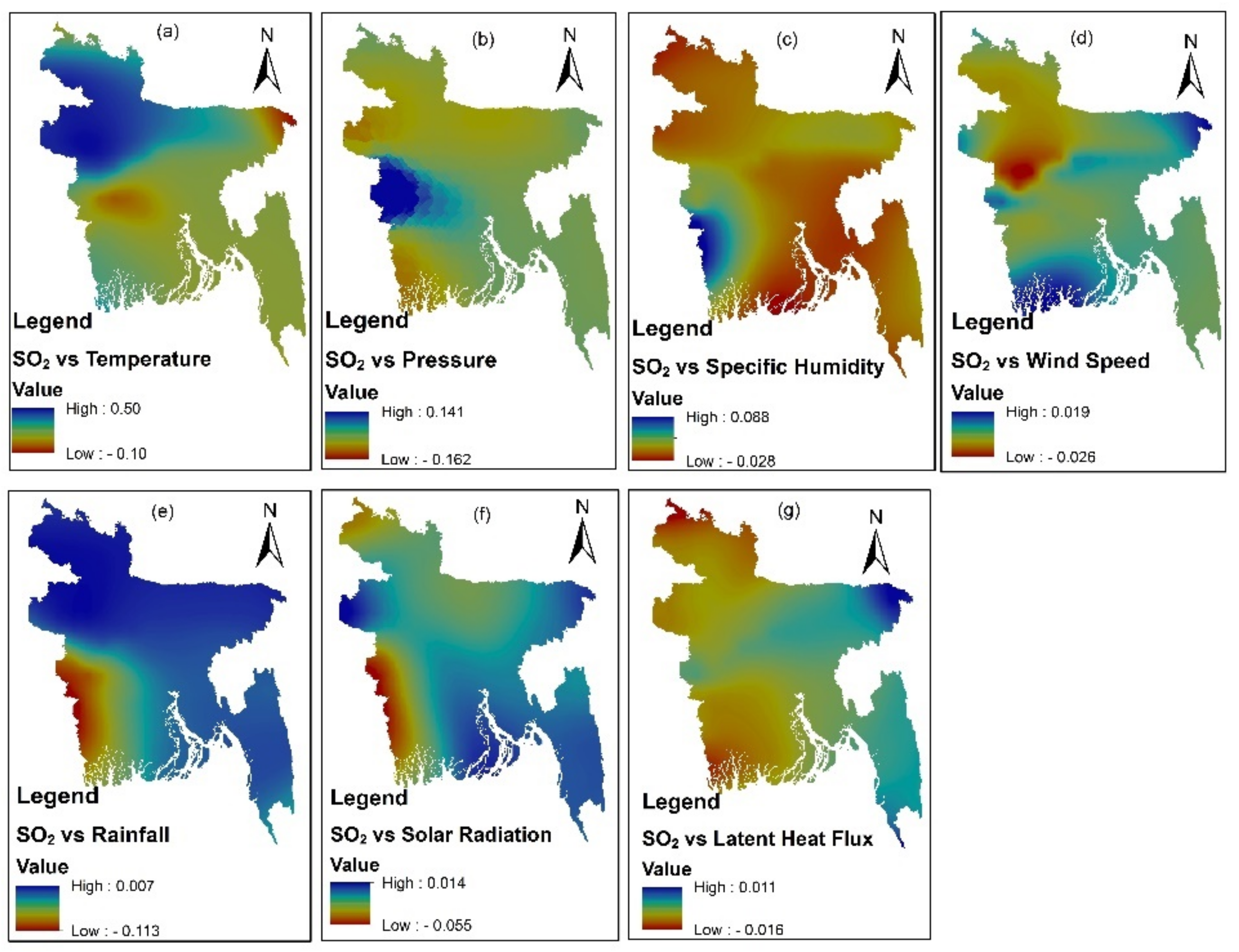
3.4.3. Spatial Relationship between SO2 and Meteorological Variables

Figure 10 shows spatial maps of the relationship between SO2 and meteorological variables over Bangladesh during 2015–2020. The relationship between SO2 and temperature was found to be positive in the northern regions of the study area, with a maximum coefficient value of 0.50 DU, whereas the central, southwestern, and eastern regions were negatively associated, with a maximum coefficient value of −0.10 DU (Figure 10a). The relationships of SO2 with pressure and specific humidity were negative throughout the country, with maximum coefficient values of −0.162 DU for pressure and −0.028 DU for specific humidity, except for a small region in the southwest, maximum positive coefficient values of 0.141 DU for pressure and 0.08 for specific humidity (Figure 10b,c). In the case of wind speed and SO2 (Figure 10d), a positive and moderate association was observed in the southwestern and eastern regions; on the other hand, the northern region showed a negative correlation, with a maximum value of −0.026 DU. The relationship between rainfall and SO2 was positively distributed in most areas with, with a maximum coefficient value of 0.007 DU, whereas it was negatively associated in the southwestern region, with a maximum coefficient value of −0.113 DU. Solar radiation and SO2 (Figure 10f) showed a positive association across most of the country, although there was a negative association in the southwestern and northernmost regions. SO2 and latent heat showed a moderate negative association across the whole the country, except in the eastern region, where there was a positive association. Overall, we observed that temperature was the most influential variable, with the highest coefficient values (0.50 DU), followed by pressure (0.14 DU) and specific humidity (0.01 DU).

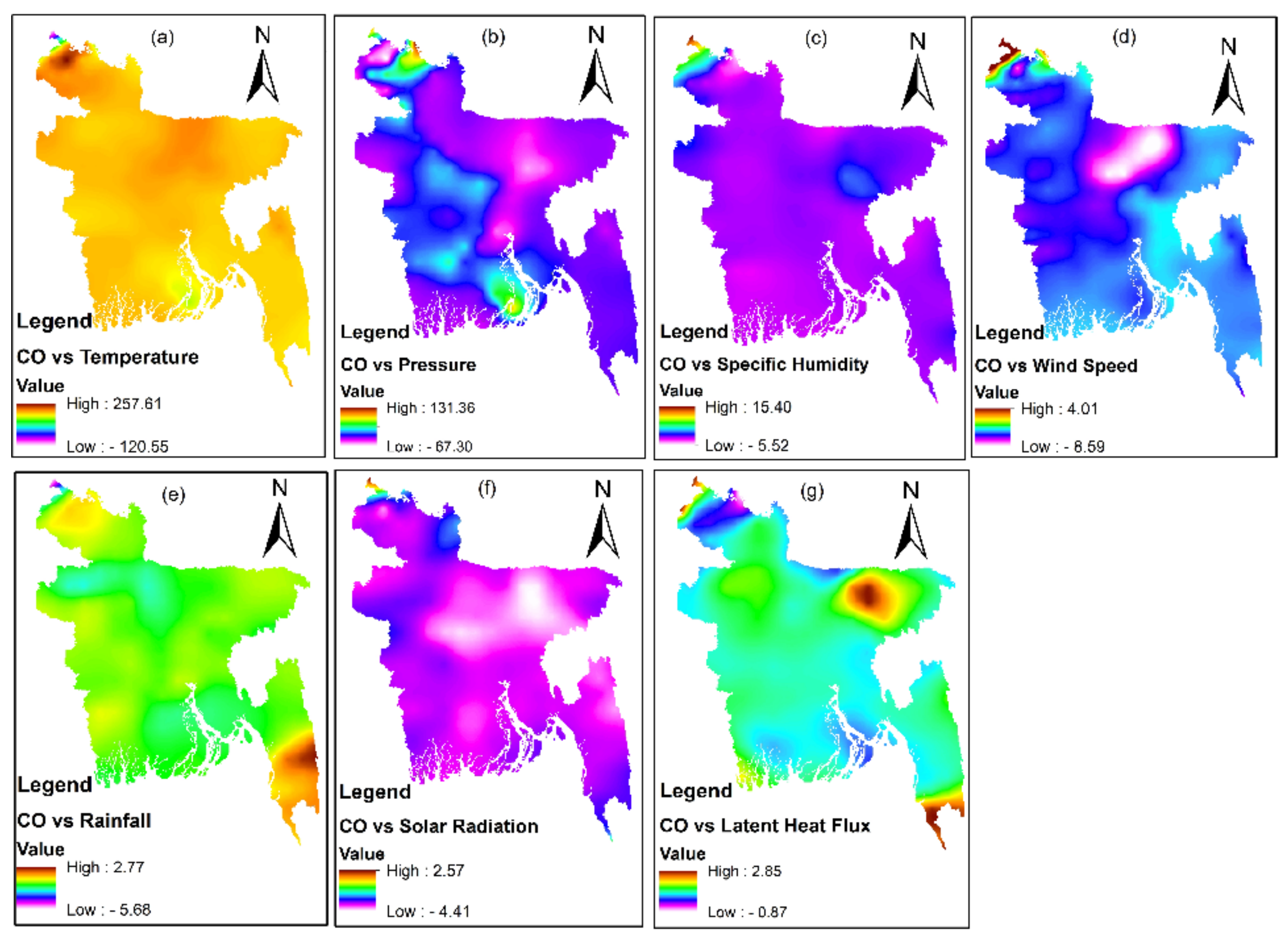
3.4.4. Spatial Relationship between CO and Meteorological Variables

Figure 11 shows the spatial maps of the relationship between CO and meteorological variables over Bangladesh during 2015–2020. The geographically varying coefficients of CO with temperature, rainfall, and latent heat flux were all positive across the majority of the study area, indicating that an increase in CO contributes to an increase in temperature, latent heat, and annual rainfall fluxes. On the other hand, coefficients of regression of the relationships between CO and the four other meteorological variables (pressure, specific humidity, wind speed, and solar radiation) were negatively associated across the study area. Overall, the coefficients of regression values were highest in association with temperature (257.61 DU), followed by pressure (131.36 DU) and specific humidity (15.40 DU), indicating that these variables are more influential in terms of variation in CO across the study area.

3.4.5. Average Coefficient Values between Air Pollutants and Meteorological Parameters

In this study, we performed analysis for each year between 2015 and 2020; however, only the results for 2020 are presented for simplification, as shown in Table 3. In 2020, the temperature showed a positive relationship with NO2 and CO but a negative relationship with O3 and SO2. The wind speed showed a positive association with all four air pollutants, but the pressure, rainfall, and latent heat exhibited negative associations with all four air pollutants. The two other parameters (specific humidity and solar radiation) showed both positive and negative relationships with air pollutants, as indicated in Table 3. Analysis of the other years showed varying coefficient values between meteorological parameters and air pollutants.
To understand the overall values of the varying coefficients from GWR modelling, the average values of the geographically varying coefficients (local) and overall R2 values for 2015–2020 were obtained as shown in Table 4. The temperature showed a positive association with NO2, SO2, and CO, with average values of 0.12 DU~3.22 × 10¹⁵ molecules/cm2, 0.182 DU, and 31.09 DU, respectively, indicating that a unit increase in temperature leads to 0.12 DU increase in NO2, while controlling the effects of other variables. In contrast, a negative association with O3, with a value of −29.02 DU, indicates that a unit increase in temperature leads to a 29.02 DU decrease in tropospheric O3 or vice-versa. These relationships are consistent with the results of other studies, except for the relationship between temperature and O3 [56,57,58]. The negative relationship between temperature and O3 might be explained by the depletion of the ozone layer due to an excess of ozone-depleting substances (ODS) over the study area [59,60]; furthermore, the production of chlorofluorocarbons (CFCs) and hydrochlorofluorocarbons (HCFCs) from air conditioning might deplete the ozone layer [61,62]. Solar radiation was negatively associated with NO2, SO2, and O3, which might be explained by chemical reactions that promote the transformation of NO2 and SO2 into nitrate and sulfate, respectively [63,64], as well as photodissociation reactions in the presence of solar radiation, which cause the breakdown of O3 into oxygen [65,66,67].
The pressure showed a positive association with all the four pollutants: NO2 by 0.43 DU, O3 by 7.21 DU, SO2 by 0.002 DU, and CO by 34.67 DU. The specific humidity, solar radiation, and latent heat showed negative associations with all three pollutants, except CO. Wind speed was positively associated with NO2 and O3 and negatively associated with CO and SO2, with different values, as shown in Table 4. Rainfall was negatively associated with all four air pollutants. However, the average coefficient values indicated that all air pollutants exhibited a significant relationship with all the meteorological variables. The overall values of R2 showed that the geographically weighted regression analysis was statistically significant.

4. Discussion

In this study, we summarized the relationships between air pollutants and meteorological variables using satellite and ground observation data over Bangladesh. The NO2 distribution in the study area showed a similar pattern as that reported in previous studies [18]; clear footprints of NO2 were found over Dhaka city and West Bengal, India, with a maximum value of 7.91 × 10¹⁵ molecules/cm2. This NO2 distribution pattern revealed NO2 hot spots in Dhaka, which were also identified as the source of NO2 according to the global emission inventory of NOx of Peaking University (PKU) (http://inventory.pku.edu.cn/home.html, (accessed on 10 January 2022), as shown in Figure 12 [68]. The emission inventory of NOx can be utilized for NO2 analysis because NOx in the troposphere mainly consists of NO and NO2, with NO2 as the secondary pollutant and NO as the primary pollutant, although NO is further oxidized to NO2 in the presence of oxidants [68,69,70]. According to previous studies [71], NO2 and NOx have similar variation trends. Figure 12a shows the total emissions (transportation, energy production, industry, residential and commercial, agricultural, deforestation, and wildfire) with transportation accounting for the highest levels of emissions in Dhaka (Figure 12b). The NO2 distribution in Dhaka was intense during weekdays and was mild during weekends according to OMI measurements (Supplementary Figure S1). NO2 distribution also presents intense seasonality, such as during the period from March to May (MAM), with a 15–40% increase over Bay of Bengal and a 15–30% increase over central India [72].
CO concentrations over the target study area and surroundings were higher, except over the Tibetan Plateau area, where values were comparatively low. The decreasing trends in surface CO since 2015 in most of Tibetan Plateau areas were attributed to the reduction in local and transported CO emissions in recent years, in line with the finding s of the present study. The average seasonal variations in air pollutants exhibited remarkable disparities over different parts of Bangladesh. During summer NO2 and O3 were moderately to highly distributed in the central and northern regions and slightly distributed over southern regions, whereas SO2 showed high distribution in southwestern regions, and CO was highly distributed in the central and western parts of the country. The distribution patterns of NO2 and O3 were similar for autumn and winter, but the highest densities were observed during winter, with 1.11 × 10¹⁶ molecules/cm2 for NO2 and 7.11 × 10¹⁸ molecules/cm2 for O3. These phenomena can be explained by the industrial emissions of NO2, which were higher in winter because brick kilns (most influential biomass-burning industry) were in production during winter in Bangladesh [19,73]. Daytime is also short during winter, resulting in less interaction with solar radiation in the atmosphere and a reduction in photodissociation reactions of O3 into oxygen, as well as the transport of O3 from the tropical to extratropical regions during winter [74]. Furthermore, air conditioning, which produces chlorofluorocarbons (CFCs) and hydrochlorofluorocarbons (HCFCs), resulting in O3 depletion [61,66], is not used in winter. SO2 showed low distribution during autumn and higher distribution during winter in most of the country. This distribution phenomenon of SO2 can be explained by the emission inventory of PKU for SO2 over Bangladesh. Figure S2 shows that the source of SO2 in the study area was mainly industry; the literature indicates that the highest quantity of industrial emissions is produced by brick kilns over Dhaka and other industrial areas [75,76]. As the atmosphere cleans itself by deposition (dry and wet) processes [77,78], in this study, we also investigated the possibility of wet and dry deposition. Precipitation can influence wet deposition by oxidizing sulfur and nitrogen compounds, resulting in improved air quality [79]; furthermore, wind speed can also accelerate dry deposition [80]. During autumn, both the precipitation and wind speed presented higher values, which accelerated wet and dry deposition, respectively, reducing concentrations of air pollutants (Figure S3). In addition, increasing wind speed can accelerate regional transportation, reducing pollutant levels in heavily polluted regions [63,81].
Trend analysis of air pollutants showed heterogeneous patterns, with increasing or decreasing rates in different parts of Bangladesh, as presented in Figure 5. NO2 and SO2 showed both increasing and decreasing trends in different parts of the country. O3 concentration increased in northern regions and decreased in central and southern areas, although the results were insignificant (p > 0.05), which may be attributed to the low signal-to-noise ratio, as well as missing information at the pixel level in raster data [82]; however, the trend analysis of O3 in this study area is not reliable. The observed negative trend of CO in Bangladesh is consistent with previous studies conducted in Asia using satellite data [83,84], which can be explained by the driving forces of global biomass burning and the reduced trends in MODIS fire counts during the last decade. In the case of meteorological trend analysis, all seven parameters showed both the positive and negative trends in different parts of Bangladesh for the last six years 2015–2020. The highest increasing trends were 0.288 K per year in temperature, 35.31 pa/year in pressure, 0.136 g/g/year in specific humidity, 0.27 m/s/year in wind speed, 0.287 mm/year in rainfall, 2.38 W/m2/year in solar radiation, and 2.52 W/m2/year in latent heat flux. The findings of the trend analysis showed a geographically varying pattern from one region to another due to the impact of monsoon climate; these results are consistent with those reported in previous studies [85,86].
GWR-based model coefficients were used to determine the degree of relationship between air pollutants and meteorological parameters. Some studies have evaluated the relationship among air pollutants and metrological variables using sole regression and generalized additive models (GAM), which do not take into account the spatial variability in relationships [19,27,28]. Complex topological features, meteorological conditions, and anthropogenic emissions affect the relationships with considerable heterogeneity in the study region. Therefore, in our study, we evaluated spatial relationships using coefficients from a GWR model. The spatial pattern of the geographically varying coefficients between air pollutants and meteorological parameters showed positive (increasing) and/or negative (decreasing) values in different regions of the study area. In this study, we considered seven meteorological parameters, including two parameters pertaining to earth surface energy balance components (Solar radiation and latent heat flux) [87] in order to understand the degree of dependency of air pollutants on different meteorological parameters.
Overall, we observed that temperature, pressure, and specific humidity were the most influential variables, with the highest coefficient values against all air pollutants, which consistent with previous studies in most areas across the globe, with some exceptions [26,27,60,71]. However, the magnitude of influence varies depending on spatial relationships across the study region. For example, NO2 regression coefficients versus temperature and specific humidity showed negative coefficient values in the central regions, whereas higher positive values were observed in the surrounding regions, indicating that the effects of meteorological indicators were more severe in surrounding regions. The overall geographically varying coefficients between temperature and CO were positive due to the heating of coal and other biomass burning in industrial areas of the study area (Figure S4), as well as local transport of CO [88].The relationship between temperature and O3 was negative, which means that the decrease with temperature might be caused by the depletion of the ozone layer due to an excess of ozone-depleting substances (ODS) over the study area [59]. However, this result is not in consistent with previous ground-based studies [56,57]. Therefore, further study is recommended with a high-resolution dataset of O3 to confirm this relationship. Wind speed was negatively associated with SO2, with an overall value of 0.85 DU, indicating that SO2 decreased by 0.85 DU with every unit increase in temperature, meaning that increased wind improved the air quality in terms of SO2. This can be explained by the transportation process caused by wind speed and is consistent with the results of previous studies [27,81].
According to the above results and discussion, this study showed that the pressure and temperature exhibited a high degree of dependency (relationship) with all four air pollutants. A moderate degree of relationship was exhibited by specific humidity, rainfall, and wind speed; rainfall showed a negative (average) relationship with all four air pollutants, i.e., rainfall improved the air quality. A low degree of association was observed for solar radiation and latent heat flux with three air pollutants and showed a noticeable degree of relationship with CO. The average yearly analysis showed that there were different values of geographically varying coefficients, even with opposite relationships between a meteorological and air pollutant in comparison with six-year average analysis. This phenomenon suggests that more high-resolution analysis, such as diurnal to yearly and long-term analysis, is necessary to develop effective air pollution control strategies. The spatial pattern analysis also showed similar phenomena for different regions, which also suggests the need for local to regional analysis with higher-resolution data. However, policy makers can be benefited from the above-indicated findings in developing suitable air pollution control policies.

5. Conclusions

In this study, we investigated the methodical relationship between four air pollutants and seven meteorological parameters by exploring their spatial patterns over Bangladesh. Overall, the results showed pressure exhibited a positive relationship with all four air pollutants (NO2, O3, SO2, and CO), i.e., an increase in the air pollutants associated with high pressure by affecting (shallowing) the atmospheric boundary layer, which promotes the formation of heavy air pollution [89,90]. High temperature was also associated with increased NO2, SO2, and CO but not O3. Increased humidity, solar radiation, and latent heat flux were associated with decreased NO2, O3, and SO2 but not CO; solar radiation was found to play an important role in the chemical reactions in the atmosphere, promoting the transformations of NO2 and SO2 into nitrate and sulfate aerosols, which suggests the need for further research on the relationship between NO2, SO2, and AOD (aerosol optical depth) in the study area. Exceptional cases were discussed in Section 4. Wind speed was positively associated with NO2 and O3 and negatively associated with other pollutants, i.e., changes in wind speed with changes in the height of the mixing layer may deteriorate (positive association) or improve (negative association) the air quality [81,90]. Rainfall was negatively associated with all four air pollutants, which accelerated wet-deposition self-cleaning of the atmosphere.
The overall distribution pattern and emission analysis revealed that the capital city area (Dhaka) was identified as the emission source/origin of NO2, SO2, and CO, with transportation emissions from NO2 and industry emissions were indicated as the most influential factors for SO2, and CO (Figure 12, Figures S2 and S4). Seasonal variations in air pollutants were influenced by the solar radiation for chemical reactions, rainfall and wind speed for self-cleaning of the atmosphere, and biomass burning for heating and/or increasing the air temperature.
Based on the results uobtained in this study, we can conclude that there is a significant and inextricable relationship between air pollutants and meteorological parameters over Bangladesh. The impact of weather conditions on air pollutants can be explained by the type of pollutant and geographical region. Policy makers can utilize these findings to set up suitable strategies and guidelines to prevent air pollution and to monitor air quality over Bangladesh. In addition, the obtained relationship between air pollutants and meteorological parameters might be influenced by the impact of climate change. Because we used 0.25 degree monthly data to investigate the relationship between air pollutants and meteorological parameters, our results might not reflect an efficient association in real-time applications. Further research is recommended to investigate the relationships between pollutants and meteorological conditions by combining the intensity of anthropogenic activities and environmental governance measures with higher spatial and temporal resolution data.

Supplementary Materials

The following supporting information can be downloaded at: https://www.mdpi.com/article/10.3390/rs14122757/s1, Figure S1. The NO2 distribution over the study area: (a) in weekdays, and (b) in weekends. Figure S2. The emission inventory of SO2 over the study area: (a) the total emissions, and (b) the industry emissions. Figure S3. The spatial distribution of wind speed and precipitation during winter and rest of the period: the first column of the figure represents the dry deposition and the second one for wet deposition. Figure S4. The emission inventory of CO over the study area: (a) the total emissions, and (b) the industry emissions.

Author Contributions

Conceptualization, M.M.R. and W.Z. (Weixiong Zhao); methodology, M.M.R.; software, M.M.R. and A.A.; formal analysis, M.M.R. and W.S.; investigation, M.M.R., W.S., and A.A.; writing—original draft preparation, M.M.R.; writing—review and editing, M.M.R., W.Z. (Weixiong Zhao), A.A., W.S., W.Z. (Weijun Zhang), and X.X.; visualization, M.M.R., A.A. and W.S.; supervision, W.Z. (Weixiong Zhao); project administration, W.Z. (Weixiong Zhao); funding acquisition, W.Z. (Weixiong Zhao). All authors have read and agreed to the published version of the manuscript.

Funding

This research was funded by the Chinese Academy of Sciences (CAS) President’s International Fellowship Initiative (PIFI) (grant 2020PE0030), the National Natural Science Foundation of China (42022051), the Youth Innovation Promotion Association CAS (Y202089), and the HFIPS Director’s Fund (YZJJ202101, BJPY2019B02, YZJJ2021QN02), and Anhui Provincial Natural Science Foundation (2108085QD181).

Acknowledgments

The first author wishes to acknowledge the intellectual contribution of the Department of Electrical and Electronic Engineering, Pabna University of Science and Technology, Pabna-6600, Bangladesh. The authors also wish to acknowledge the Earth Data portal of NASA and the CASE project of the Ministry of Environment and Forestry, Bangladesh, for providing data.

Conflicts of Interest

The authors declare no conflict of interest.

References

  1. Kampa, M.; Castanas, E. Human health effects of air pollution. Environ. Pollut. 2008, 151, 362–367. [Google Scholar] [CrossRef] [PubMed]
  2. Wang, K.; Wang, W.; Wang, W.; Jiang, X.; Yu, T.; Ciren, P. Spatial assessment of health economic losses from exposure to ambient pollutants in China. Remote Sens. 2020, 12, 790. [Google Scholar] [CrossRef] [Green Version]
  3. Guan, W.J.; Zheng, X.Y.; Chung, K.F.; Zhong, N.S. Impact of air pollution on the burden of chronic respiratory diseases in China: Time for urgent action. Lancet 2016, 388, 1939–1951. [Google Scholar] [CrossRef]
  4. Liu, C.; Chen, R.; Sera, F.; Vicedo-Cabrera, A.M.; Guo, Y.; Tong, S.; Coelho, M.S.Z.S.; Saldiva, P.H.N.; Lavigne, E.; Matus, P.; et al. Ambient Particulate Air Pollution and Daily Mortality in 652 Cities. N. Engl. J. Med. 2019, 381, 705–715. [Google Scholar] [CrossRef] [PubMed]
  5. Vineis, P.; Forastiere, F.; Hoek, G.; Lipsett, M. Outdoor air pollution and lung cancer: Recent epidemiologic evidence. Int. J. Cancer 2004, 111, 647–652. [Google Scholar] [CrossRef] [PubMed]
  6. Hoek, G.; Krishnan, R.M.; Beelen, R.; Peters, A.; Ostro, B.; Brunekreef, B.; Kaufman, J.D. Long-term air pollution exposure and cardio-respiratory mortality: A review. Environ. Health A Glob. Access Sci. Source 2013, 12, 43. [Google Scholar] [CrossRef] [PubMed] [Green Version]
  7. Lelieveld, J.; Evans, J.S.; Fnais, M.; Giannadaki, D.; Pozzer, A. The contribution of outdoor air pollution sources to premature mortality on a global scale. Nature 2015, 525, 367–371. [Google Scholar] [CrossRef]
  8. Buoli, M.; Grassi, S.; Caldiroli, A.; Carnevali, G.S.; Mucci, F.; Iodice, S.; Cantone, L.; Pergoli, L.; Bollati, V. Is there a link between air pollution and mental disorders? Environ. Int. 2018, 118, 154–168. [Google Scholar] [CrossRef]
  9. Duncan, B.N.; Prados, A.I.; Lamsal, L.N.; Liu, Y.; Streets, D.G.; Gupta, P.; Hilsenrath, E.; Kahn, R.A.; Nielsen, J.E.; Beyersdorf, A.J.; et al. Satellite data of atmospheric pollution for U.S. air quality applications: Examples of applications, summary of data end-user resources, answers to FAQs, and common mistakes to avoid. Atmos. Environ. 2014, 94, 647–662. [Google Scholar] [CrossRef] [Green Version]
  10. Sheehan, P.; Cheng, E.; English, A.; Sun, F. China’s response to the air pollution shock. Nat. Clim. Change 2014, 4, 306–309. [Google Scholar] [CrossRef]
  11. Gao, J.; Tian, H.; Cheng, K.; Lu, L.; Zheng, M.; Wang, S.; Hao, J.; Wang, K.; Hua, S.; Zhu, C.; et al. The variation of chemical characteristics of PM 2.5 and PM 10 and formation causes during two haze pollution events in urban Beijing, China. Atmos. Environ. 2015, 107, 1–8. [Google Scholar] [CrossRef]
  12. Liu, J.; Mauzerall, D.L.; Chen, Q.; Zhang, Q.; Song, Y.; Peng, W.; Klimont, Z.; Qiu, X.; Zhang, S.; Hu, M.; et al. Air pollutant emissions from Chinese households: A major and underappreciated ambient pollution source. Proc. Natl. Acad. Sci. USA 2016, 113, 7756–7761. [Google Scholar] [CrossRef] [Green Version]
  13. Editorial Cleaner air for China. Nat. Geosci. 2019, 12, 497. [CrossRef]
  14. Tilt, B. China’s air pollution crisis: Science and policy perspectives. Environ. Sci. Policy 2019, 92, 275–280. [Google Scholar] [CrossRef]
  15. He, J.; Gong, S.; Yu, Y.; Yu, L.; Wu, L.; Mao, H.; Song, C.; Zhao, S.; Liu, H.; Li, X.; et al. Air pollution characteristics and their relation to meteorological conditions during 2014–2015 in major Chinese cities. Environ. Pollut. 2017, 223, 484–496. [Google Scholar] [CrossRef]
  16. Begum, B.A.; Hopke, P.K.; Markwitz, A. Air pollution by fine particulate matter in Bangladesh. Atmos. Pollut. Res. 2013, 4, 75–86. [Google Scholar] [CrossRef] [Green Version]
  17. Muntaseer Billah Ibn Azkar, M.A.; Chatani, S.; Sudo, K. Simulation of urban and regional air pollution in Bangladesh. J. Geophys. Res. Atmos. 2012, 117, 16509. [Google Scholar] [CrossRef] [Green Version]
  18. Ul-Haq, Z.; Tariq, S.; Ali, M. Tropospheric NO2 trends over south Asia during the last decade (2004–2014) using OMI Data. Adv. Meteorol. 2015, 2015, 959284. [Google Scholar] [CrossRef] [Green Version]
  19. Pavel, M.R.S.; Zaman, S.U.; Jeba, F.; Islam, M.S.; Salam, A. Long-Term (2003–2019) Air Quality, Climate Variables, and Human Health Consequences in Dhaka, Bangladesh. Front. Sustain. Cities 2021, 3, 681759. [Google Scholar] [CrossRef]
  20. Elminir, H.K. Dependence of urban air pollutants on meteorology. Sci. Total Environ. 2005, 350, 225–237. [Google Scholar] [CrossRef]
  21. Fu, Y.; Gao, H.; Liao, H.; Tian, X. Spatiotemporal variations and uncertainty in crop residue burning emissions over North China plain: Implication for atmospheric co2 simulation. Remote Sens. 2021, 13, 3880. [Google Scholar] [CrossRef]
  22. Li, R.; Wang, Z.; Cui, L.; Fu, H.; Zhang, L.; Kong, L.; Chen, W.; Chen, J. Air pollution characteristics in China during 2015–2016: Spatiotemporal variations and key meteorological factors. Sci. Total Environ. 2019, 648, 902–915. [Google Scholar] [CrossRef] [PubMed]
  23. Zhou, H.; Yu, Y.; Gu, X.; Wu, Y.; Wang, M.; Yue, H.; Gao, J.; Lei, R.; Ge, X. Characteristics of air pollution and their relationship with meteorological parameters: Northern versus southern cities of China. Atmosphere 2020, 11, 253. [Google Scholar] [CrossRef] [Green Version]
  24. Cai, W.; Li, K.; Liao, H.; Wang, H.; Wu, L. Weather conditions conducive to Beijing severe haze more frequent under climate change. Nat. Clim. Change 2017, 7, 257–262. [Google Scholar] [CrossRef]
  25. Turalioglu, S.O. Relationship Between Air Pollutants and Some Meteorological Parameters in Erzurum, Turkey. In Global Warming, Green Energy and Technology; Springer: New York, NY, USA, 2010; Volume 31, ISBN 9781441910165. [Google Scholar]
  26. Jayamurugan, R.; Kumaravel, B.; Palanivelraja, S.; Chockalingam, M.P. Influence of Temperature, Relative Humidity and Seasonal Variability on Ambient Air Quality in a Coastal Urban Area. Int. J. Atmos. Sci. 2013, 2013, 264046. [Google Scholar] [CrossRef] [Green Version]
  27. Liu, Y.; Zhou, Y.; Lu, J. Exploring the relationship between air pollution and meteorological conditions in China under environmental governance. Sci. Rep. 2020, 10, 14518. [Google Scholar] [CrossRef]
  28. Di, Y.H.; Li, R.R. Correlation analysis of AQI characteristics and meteorological conditions in heating season. IOP Conf. Ser. Earth Environ. Sci. 2019, 242, 022067. [Google Scholar] [CrossRef]
  29. Hou, K.; Xu, X. Evaluation of the influence between local meteorology and air quality in Beijing using generalized additive models. Atmosphere 2022, 13, 24. [Google Scholar] [CrossRef]
  30. Foody, G.M. Geographical weighting as a further refinement to regression modelling: An example focused on the NDVI-rainfall relationship. Remote Sens. Environ. 2003, 88, 283–293. [Google Scholar] [CrossRef]
  31. Hanna, S.R. Handbook on Atmospheric Diffusion Models; U.S. Department of Energy: Washington, DC, USA, 1981; Volume 11223, ISBN 0870791273.
  32. Barua, D.K. The active delta of the ganges-brahmaputra rivers: Dynamics of its present formations. Mar. Geod. 1997, 20, 1–12. [Google Scholar] [CrossRef]
  33. Rahman, M.; Ghosh, T.; Salehin, M.; Ghosh, A.; Haque, A.; Hossain, M.A.; Das, S.; Hazra, S.; Islam, N.; Sarker, M.H.; et al. Ganges-Brahmaputra-Meghna Delta, Bangladesh and India: A Transnational Mega-Delta. In Deltas in the Anthropocene; Palgrave Macmillan: Cham, Switzerland, 2020; pp. 23–51. ISBN 9783030235161. [Google Scholar]
  34. Becker, M.; Papa, F.; Karpytchev, M.; Delebecque, C.; Krien, Y.; Khan, J.U.; Ballu, V.; Durand, F.; Le Cozannet, G.; Islam, A.K.M.S.; et al. Water level changes, subsidence, and sea level rise in the Ganges-Brahmaputra-Meghna delta. Proc. Natl. Acad. Sci. USA 2020, 117, 1867–1876. [Google Scholar] [CrossRef]
  35. Bari, S.H.; Hussain, M.M.; Husna, N.E.A. Rainfall variability and seasonality in northern Bangladesh. Theor. Appl. Climatol. 2017, 129, 995–1001. [Google Scholar] [CrossRef]
  36. Harzallah, A.; Sadourny, R. Observed lead-lag relationships between Indian summer monsoon and some meteorological variables. Clim. Dyn. 1997, 13, 635–648. [Google Scholar] [CrossRef]
  37. Nickolay, A.; Krotkov, L.N.; Lamsal, S.; Marchenko, V.; Celarier, A.E.; Bucsela, E.J.; William, H.; Swartz, J.J.; OMI Core Team. OMI/Aura NO2 Cloud-Screened Total and Tropospheric Column L3 Global Gridded 0.25 Degree × 0.25 Degree V3; NASA Goddard Space Flight Center, Goddard Earth Sciences Data and Information Services Center (GES DISC): Greenbelt, MD, USA, 2019.
  38. Li, C.; Nickolay, A.; Krotkov, P.L. OMI/Aura Sulfur Dioxide (SO2) Total Column L3 1 Day Best Pixel in 0.25 Degree × 0.25 Degree V3; Goddard Earth Sciences Data and Information Services Center (GES DISC): Greenbelt, MD, USA, 2020. [Google Scholar]
  39. Veefkind, P. OMI/Aura Ozone (O3) DOAS Total Column L3 1 Day 0.25 degree × 0.25 Degree V3; Goddard Earth Sciences Data and Information Services Center (GES DISC): Greenbelt, MD, USA, 2012. [Google Scholar]
  40. MOPITT Team. MOPITT Measurement of Pollution in the Troposphere; MOPITT Team: Boulder, CO, USA, 1996. [Google Scholar]
  41. Barret, B.; De Mazière, M.; Mahieu, E. Ground-based FTIR measurements of CO from the Jungfraujoch: Characterisation and comparison with in situ surface and MOPITT data. Atmos. Chem. Phys. 2003, 3, 2217–2223. [Google Scholar] [CrossRef] [Green Version]
  42. Rodell, M.; Houser, P.R.; Jambor, U.; Gottschalck, J.; Mitchell, K.; Meng, C.J.; Arsenault, K.; Cosgrove, B.; Radakovich, J.; Bosilovich, M.; et al. The Global Land Data Assimilation System. Bull. Am. Meteorol. Soc. 2004, 85, 381–394. [Google Scholar] [CrossRef] [Green Version]
  43. Beaudoing, H.; Rodell, N. GLDAS Noah Land Surface Model L4 Monthly 0.25 × 0.25 degree V2.1. Goddard Earth Sciences Data and Information Services Center (GES DISC): Greenbelt, Maryland, USA. Available online: https://disc.gsfc.nasa.gov/datasets/GLDAS_NOAH025_3H_2.1/summary (accessed on 20 November 2021).
  44. Li, B.; Beaudoing, H.; Rodell, N.M. GLDAS Catchment Land Surface Model L4 Daily 0.25 × 0.25 Degree V2.0; Goddard Earth Sciences Data and Information Services Center (GES DISC): Greenbelt, MD, USA, 2014. [Google Scholar]
  45. Huffman, G.J.; Bolvin, D.T.; Nelkin, E.J. TRMM (TMPA) Precipitation L3 1 Day 0.25 Degree × 0.25 Degree V7; Savtchenko, A., Ed.; Goddard Earth Sciences Data and Information Services Center (GES DISC): Greenbelt, MD, USA, 2019. [Google Scholar]
  46. Chen, Y.; Yang, K.; Qin, J.; Zhao, L.; Tang, W.; Han, M. Evaluation of AMSR-E retrievals and GLDAS simulations against observations of a soil moisture network on the central Tibetan Plateau. J. Geophys. Res. Atmos. 2013, 118, 4466–4475. [Google Scholar] [CrossRef]
  47. Nakaya, T.; Fotheringham, A.S.; Charlton, M.; Brunsdon, C. Semiparametric geographically weighted generalised linear modelling in GWR 4.0. In Proceedings of the 10th International Conference on GeoComputation, University of New South Wales, Sydney, Australia, 30 November–2 December 2009; pp. 1–5. [Google Scholar]
  48. Nakaya, T. Windows Application for Geographically Weighted Regression Modelling; Department of Geography, Ritsumeikan University: Kyoto, Japan, 2016; Available online: https://gwr.maynoothuniversity.ie/gwr4-software/ (accessed on 28 October 2021).
  49. Nakaya, T.; Fotheringham, A.S.; Brunsdon, C.; Charlton, M. Geographically weighted Poisson regression for disease association mapping. Stat. Med. 2005, 24, 2695–2717. [Google Scholar] [CrossRef] [Green Version]
  50. Calvert, J.G. Glossary of atmospheric chemistry terms. Pure Appl. Chem. 1990, 62, 2167–2219. [Google Scholar] [CrossRef] [Green Version]
  51. Dobson Unit—Wikipedia. Available online: https://en.wikipedia.org/wiki/Dobson_unit (accessed on 15 January 2022).
  52. Dobson Unit. Available online: https://www.temis.nl/general/dobsonunit.php (accessed on 15 January 2022).
  53. Rahman, M.M.; Mahamud, S.; Thurston, G.D. Recent spatial gradients and time trends in Dhaka, Bangladesh, air pollution and their human health implications. J. Air Waste Manag. Assoc. 2019, 69, 478–501. [Google Scholar] [CrossRef]
  54. Mahmud, K.; Gope, K.; Chowdhury, S.M.R. Possible Causes & Solutions of Traffic Jam and Their Impact on the Economy of Dhaka City. J. Manag. Sustain. 2012, 2, 112–135. [Google Scholar] [CrossRef]
  55. Zhou, Z.; Zhou, Y.; Ge, X. Nitrogen Oxide Emission, Economic Growth and Urbanization in China: A Spatial Econometric Analysis. IOP Conf. Ser. Mater. Sci. Eng. 2018, 301, 012126. [Google Scholar] [CrossRef]
  56. Zhao, M.; Liu, Y.; Gyilbag, A. Assessment of Meteorological Variables and Air Pollution Affecting COVID-19 Cases in Urban Agglomerations: Evidence from China. Int. J. Environ. Res. Public Health 2022, 19, 531. [Google Scholar] [CrossRef]
  57. Ilić, P.; Popović, Z.; Nešković Markić, D. Assessment of Meteorological Effects and Ozone Variation in Urban Area. Ecol. Chem. Eng. 2020, 27, 373–385. [Google Scholar] [CrossRef]
  58. Khiem, M.; Ooka, R.; Huang, H.; Hayami, H.; Yoshikado, H.; Kawamoto, Y. Analysis of the Relationship between Changes in Meteorological Conditions and the Variation in Summer Ozone Levels over the Central Kanto Area. Adv. Meteorol. 2010, 2010, 349248. [Google Scholar] [CrossRef] [Green Version]
  59. Lu, X.; Zhang, L.; Shen, L. Meteorology and Climate Influences on Tropospheric Ozone: A Review of Natural Sources, Chemistry, and Transport Patterns. Curr. Pollut. Reports 2019, 5, 238–260. [Google Scholar] [CrossRef] [Green Version]
  60. Nurjanah, A.; Arifin, M.; Hayashi, T. Ozone Depletion and its Impacts on Life of Asian Countries; Gifu University: Gifu, Japan, 2008. [Google Scholar]
  61. Okoro, E.C.; Okeke, F.N.; Omeje, L.C. Investigating Contributions of Total Column Ozone Variation on Some Meteorological Parameters in Nigeria. Atmos. Clim. Sci. 2022, 12, 132–149. [Google Scholar] [CrossRef]
  62. Automobile Air Conditioners and Chlorofluorocarbons (CFCs). Available online: https://p2infohouse.org/ref/01/00038.htm (accessed on 18 January 2022).
  63. Ozone-Depleting Substances|US EPA. Available online: https://www.epa.gov/ozone-layer-protection/ozone-depleting-substances (accessed on 18 January 2022).
  64. Lin, C.A.; Chen, Y.C.; Liu, C.Y.; Chen, W.T.; Seinfeld, J.H.; Chou, C.C.K. Satellite-derived correlation of SO2, NO2, and aerosol optical depth with meteorological conditions over East Asia from 2005 to 2015. Remote Sens. 2019, 11, 1738. [Google Scholar] [CrossRef] [Green Version]
  65. Khoder, M.I. Atmospheric conversion of sulfur dioxide to particulate sulfate and nitrogen dioxide to particulate nitrate and gaseous nitric acid in an urban area. Chemosphere 2002, 49, 675–684. [Google Scholar] [CrossRef]
  66. Photodissociation—Wikipedia. Available online: https://en.wikipedia.org/wiki/Photodissociation (accessed on 20 January 2022).
  67. Environmental effects of ozone depletion and its interactions with climate change: 2002 assessment. Executive summary. Photochem. Photobiol. Sci. 2003, 2, 1–4. [Google Scholar] [CrossRef] [Green Version]
  68. Sun, Y.; Yin, H.; Cheng, Y.; Zhang, Q.; Zheng, B.; Notholt, J.; Lu, X.; Liu, C.; Tian, Y.; Liu, J. Quantifying variability, source, and transport of CO in the urban areas over the Himalayas and Tibetan Plateau. Atmos. Chem. Phys. 2021, 21, 9201–9222. [Google Scholar] [CrossRef]
  69. Jamali, S.; Klingmyr, D.; Tagesson, T. Global-scale patterns and trends in tropospheric no2 concentrations, 2005–2018. Remote Sens. 2020, 12, 3526. [Google Scholar] [CrossRef]
  70. Huang, T.; Zhu, X.; Zhong, Q.; Yun, X.; Meng, W.; Li, B.; Ma, J.; Zeng, E.Y.; Tao, S. Spatial and Temporal Trends in Global Emissions of Nitrogen Oxides from 1960 to 2014. Environ. Sci. Technol. 2017, 51, 7992–8000. [Google Scholar] [CrossRef] [PubMed]
  71. Beevers, S.D.; Westmoreland, E.; de Jong, M.C.; Williams, M.L.; Carslaw, D.C. Trends in NOx and NO2 emissions from road traffic in Great Britain. Atmos. Environ. 2012, 54, 107–116. [Google Scholar] [CrossRef]
  72. Logan, J.A. Nitrogen Oxides in the Troposphere’ Global and Regional Budget. J. Geophys. Res. 1983, 88, 10785–10807. [Google Scholar] [CrossRef]
  73. Jena, C.; Ghude, S.D.; Pfister, G.G.; Chate, D.M.; Kumar, R.; Beig, G.; Surendran, D.E.; Fadnavis, S.; Lal, D.M. Influence of springtime biomass burning in South Asia on regional ozone (O3): A model based case study. Atmos. Environ. 2015, 100, 37–47. [Google Scholar] [CrossRef]
  74. ICIMOD. FACT SHEET-Brick Sector in Bangladesh; International Centre for Integrated Mountain Development (ICIMOD): Kathmandu, Nepal, 2019; Available online: https://lib.icimod.org/record/34681 (accessed on 20 December 2021).
  75. Guttikunda, S.K.; Begum, B.A.; Wadud, Z. Particulate pollution from brick kiln clusters in the Greater Dhaka region, Bangladesh. Air Qual. Atmos. Health 2013, 6, 357–365. [Google Scholar] [CrossRef]
  76. Alam, H. Brick Kilns Top Polluter. Available online: https://www.thedailystar.net/frontpage/news/brick-kilns-top-polluter-1701871 (accessed on 25 December 2021).
  77. Wu, Y.; Liu, J.; Zhai, J.; Cong, L.; Wang, Y.; Ma, W.; Zhang, Z.; Li, C. Comparison of dry and wet deposition of particulate matter in near-surface waters during summer. PLoS ONE 2018, 13, e0199241. [Google Scholar] [CrossRef]
  78. Lin, J.J.; Noll, K.E.; Holsen, T.M. Dry deposition velocities as a function of particle size in the ambient atmosphere. Aerosol Sci. Technol. 1994, 20, 239–252. [Google Scholar] [CrossRef] [Green Version]
  79. Wałaszek, K.; Kryza, M.; Dore, A.J. The impact of precipitation on wet deposition of sulphur and nitrogen compounds. Ecol. Chem. Eng. S 2013, 20, 733–745. [Google Scholar] [CrossRef] [Green Version]
  80. Zannetti, P. Dry and Wet Deposition. In Air Pollution Modeling; Springer: Boston, MA, USA, 1990; pp. 249–262. [Google Scholar] [CrossRef]
  81. Oleniacz, R.; Bogacki, M.; Szulecka, A.; Rzeszutek, M.; Mazur, M. Assessing the Impact of Wind Speed and Mixing-Layer Height on Air Quality in Krakow (Poland) in the Years 2014–2015. J. Civ. Eng. Environ. Archit. 2016, 63, 315–342. [Google Scholar] [CrossRef] [Green Version]
  82. Lubiński, P. Analysis of extremely low signal-to-noise ratio data from INTEGRAL/PICsIT. Astron. Astrophys. 2009, 496, 557–576. [Google Scholar] [CrossRef]
  83. Zhang, X.; Liu, J.; Han, H.; Zhang, Y.; Jiang, Z.; Wang, H.; Meng, L.; Li, Y.C.; Liu, Y. Satellite-observed variations and trends in carbon monoxide over Asia and their sensitivities to biomass burning. Remote Sens. 2020, 12, 830. [Google Scholar] [CrossRef] [Green Version]
  84. Zheng, B.; Chevallier, F.; Ciais, P.; Yin, Y.; Deeter, M.N.; Worden, H.M.; Wang, Y.; Zhang, Q.; He, K. Rapid decline in carbon monoxide emissions and export from East Asia between years 2005 and 2016. Environ. Res. Lett. 2018, 13, 044007. [Google Scholar] [CrossRef] [Green Version]
  85. Bhuyan, M.D.I.; Islam, M.M.; Bhuiyan, M.E.K. A Trend Analysis of Temperature and Rainfall to Predict Climate Change for Northwestern Region of Bangladesh. Am. J. Clim. Change 2018, 7, 115–134. [Google Scholar] [CrossRef] [Green Version]
  86. Saimi, F.M.; Hamzah, F.M.; Toriman, M.E.; Jaafar, O.; Tajudin, H. Trend and linearity analysis of meteorological parameters in peninsular Malaysia. Sustainability 2020, 12, 9533. [Google Scholar] [CrossRef]
  87. Rahman, M.M.; Zhang, W.; Wang, K. Assessment on surface energy imbalance and energy partitioning using ground and satellite data over a semi-arid agricultural region in north China. Agric. Water Manag. 2019, 213, 298–308. [Google Scholar] [CrossRef]
  88. Bei, N.; Li, G.; Huang, R.J.; Cao, J.; Meng, N.; Feng, T.; Liu, S.; Zhang, T.; Zhang, Q.; Molina, L.T. Typical synoptic situations and their impacts on the wintertime air pollution in the Guanzhong basin, China. Atmos. Chem. Phys. 2016, 16, 7373–7387. [Google Scholar] [CrossRef] [Green Version]
  89. Ning, G.; Wang, S.; Yim, S.H.L.; Li, J.; Hu, Y.; Shang, Z.; Wang, J.; Wang, J. Impact of low-pressure systems on winter heavy air pollution in the northwest Sichuan Basin, China. Atmos. Chem. Phys. 2018, 18, 13601–13615. [Google Scholar] [CrossRef] [Green Version]
  90. Schäfer, K.; Emeis, S.; Hoffmann, H.; Jahn, C. Influence of mixing layer height upon air pollution in urban and sub-urban areas. Meteorol. Z. 2006, 15, 647–658. [Google Scholar] [CrossRef] [Green Version]
Figure 1. Geographical location of the study area, along with its surroundings. The background of the figure shows the terrain.
Remotesensing 14 02757 g001
Figure 2. Comparison of the OMI measured column densities and the in situ measured mixing ratios: (ad) NO2; (e,f) SO2.
Remotesensing 14 02757 g002
Figure 3. Mean values of air pollutants from 2015 to 2020 over Bangladesh and its surroundings: (a) NO2, (b) O3, (c) SO2, and (d) CO.
Remotesensing 14 02757 g003
Figure 4. Six-year (2015–2020) average seasonal variations in air pollutants. (ac) NO2, (df) O3, (gi) SO2, (jl) CO.
Remotesensing 14 02757 g004
Figure 5. Trend analysis of four air pollutants over Bangladesh (the first row of each column shows the slope, and the second row of each column shows the p value).
Remotesensing 14 02757 g005
Figure 6. Trend analysis of meteorological parameters over Bangladesh for the period of 2015–2020: (a) temperature, (b) pressure, (c) specific humidity, (d) wind speed, (e) rainfall, (f) solar radiation, and (g) latent heat flux.
Remotesensing 14 02757 g006
Figure 7. The p values for the trend analysis of meteorological parameters over Bangladesh in the period of 2015–2020: (a) temperature, (b) pressure, (c) specific humidity, (d) wind speed, (e) rainfall, (f) solar radiation, and (g) latent heat flux.
Remotesensing 14 02757 g007
Figure 8. Spatial representation of the relationship between NO2 and meteorological variables using the geographically varying coefficients from GWR modelling over Bangladesh during 2015–2020: (a) temperature, (b) pressure, (c) specific humidity, (d) wind speed, (e) rainfall, (f) solar radiation, and (g) latent heat flux.
Remotesensing 14 02757 g008
Figure 9. Spatial representation of the relationship between O3 and meteorological variables using the geographically varying coefficients from GWR modelling over Bangladesh during 2015–2020: (a) temperature, (b) pressure, (c) specific humidity, (d) wind speed, (e) rainfall, (f) solar radiation, and (g) latent heat flux.
Remotesensing 14 02757 g009
Figure 10. Spatial representation of the relationship between SO2 and meteorological variables using the geographically varying coefficients from GWR modelling over Bangladesh during 2015–2020: (a) temperature, (b) pressure, (c) specific humidity, (d) wind speed, (e) rainfall, (f) solar radiation, and (g) latent heat flux.
Remotesensing 14 02757 g010
Figure 11. Spatial representation of the relationship between CO and meteorological variables using the geographically varying coefficients from GWR modelling over Bangladesh during 2015–2020: (a) temperature, (b) pressure, (c) specific humidity, (d) wind speed, (e) rainfall, (f) solar radiation, and (g) latent heat flux.
Remotesensing 14 02757 g011
Figure 12. Emission inventory of NOx over the target study area: (a) total emissions, (b) transportation emissions.
Remotesensing 14 02757 g012
Table 1. Key specifications of the data utilized in this study.
Data Source/PlatformParameterDefault Units *Spatial ResolutionTemporal ResolutionWeb Link
Ozone Monitoring Instrument (OMI)/AuraNitrogen dioxide (NO2)Molecules/cm20.25° × 0.25°Daily **https://giovanni.gsfc.nasa.gov/giovanni (accessed on 25 October 2021)
Ozone (O3)Dobson Units (DU)0.25° × 0.25°Daily **
Sulfur dioxide (SO2)Dobson Units (DU)0.25° × 0.25°Daily **
Measurement of Pollution in the Troposphere (MOPITT)/TerraCarbon monoxide (CO)Molecules/cm21.0° × 1.0°Monthly
Global Land Data Assimilation System (GLDAS)/Noah **Temperature (T)Kelvin0.25° × 0.25°Monthly
Pressure (P)Pascal (Pa)0.25° × 0.25°Monthly
Specific humidity (SH)kg/kg0.25° × 0.25°Monthly
Wind speed (WS)m/s0.25° × 0.25°Monthly
Tropical Rainfall Measuring Mission (TRMM)Rainfall (Rf)Mm0.25° × 0.25°Monthly
Global Land Data Assimilation System/Noah ***Net solar radiation (Rs)W/m20.25° × 0.25°Monthly
Latent heat flux (LE)W/m20.25° × 0.25°Monthly
* Default units are the units as obtained from the satellite/reanalysis images. ** Daily data were averaged into monthly values. *** Noah stands for National Centers for Environmental Prediction/Oregon State University/Air Force/Hydrologic Research Lab.
Table 2. Conversion factors and molecular weights for the air pollutants at standard pressure and temperature.
Air PollutantConversion FactorMolecular Weight
Ozone (O3)1 ppb * = 1.96 µg/m348.00 g/mol
Nitrogen dioxide (NO2)1 ppb = 1.88 µg/m346.01 g/mol
Sulfur dioxide (SO2)1 ppb = 2.62 µg/m364.07 g/mol
Carbon monoxide (CO)1 ppb = 1.15 µg/m32.01 g/mol
* According to convention of the air quality community, 1 µg/m3 = 0.05 ppb.
Table 3. Average values of geographically varying coefficients in the study area as obtained from GWR modelling over Bangladesh in 2020.
Variable Names (Units)NO2 (DU *)O3 (DU)SO2 (DU)CO (DU *)
Temperature (K)0.95−132.30−1.300.26
Pressure (Pa)−0.19−2.50−0.11−0.02
Specific Humidity (g/g)−0.06−3.21−0.080.01
Wind Speed (m/s)0.011.130.010.002
Rainfall (mm)−0.01−0.53−0.002−0.002
Solar Radiation (W/m2)0.02−1.42−0.01−0.003
Latent Heat Flux (W/m2)−0.01−0.52−0.0030.0003
R20.900.930.760.94
* The default units (molecules/cm2) of raster images for NO2 and CO were converted into DU (1 DU = 2.69 × 10¹⁶ molecules/cm2).
Table 4. Average values of geographically varying coefficients as obtained from GWR modelling over Bangladesh in the period of 2015–2020.
Variable Names (Units)NO2 (DU *)O3 (DU)SO2 (DU)CO (DU *)
Temperature (K)0.12−29.020.18231.09
Pressure (Pa)0.437.210.00234.67
Specific Humidity (g/g)−0.04−1.09−0.0015.93
Wind Speed (m/s)0.020.57−0.002−0.85
Rainfall (mm)−0.01−0.82−0.018−1.79
Solar Radiation (W/m2)−0.02−0.62−0.0120.62
Latent Heat Flux (W/m2)−0.01−0.15−0.0021.12
R20.900.930.760.94
* The default units (molecules/cm2) of raster images for NO2 and CO were converted into DU (1 DU = 2.69 × 10¹⁶ Molecules/cm2).
Publisher’s Note: MDPI stays neutral with regard to jurisdictional claims in published maps and institutional affiliations.

