
Evaluating the Long-Term Health and Economic Impacts of Central Residential Air Filtration for Reducing Premature Mortality Associated with Indoor Fine Particulate Matter (PM2.5) of Outdoor Origin


Abstract
:1. Introduction
2. Methods
2.1. Health and Economic Impact Modeling Methods
2.1.1. Estimating Health and Economic Endpoints Associated with Air Pollution
- Δyi = change in annual health endpoint (per person per year)
- y0 = annual baseline prevalence of illness (per person per year)
- βi = C-R endpoint effect estimate for pollutant i (e.g., per μg/m3 of pollutant i)
- Δxi = change in concentration or exposure (e.g., μg/m3 of pollutant i)
- DALYs = disability-adjusted life-years associated with change in health endpoint (per person per year)
- = DALYs lost per incidence
- Ai = value of avoided morbidity or mortality endpoint ($ per person per year)
- $i = monetary value per incident ($/incident)
2.1.2. C-R Endpoint Effect Estimates for Long-Term PM2.5 Mortality
2.1.3. Response Functions for Indoor PM2.5 of Outdoor Origin
- βi,indoor = C-R endpoint effect estimate for a change in long-term indoor PM2.5 concentration (per μg/m3)
- ΔCin,exposure = change in indoor PM2.5 exposure concentration (μg/m3)
- ΔCin = change in indoor PM2.5 concentration (µg/m3)
- Ptime,indoor = fraction of time spend inside a residence (0.7)
2.1.4. Modified Response Functions for Indoor PM2.5 of Outdoor Origin
- = endpoint effect estimate for premature mortality associated with outdoor PM2.5 (% per μg/m3)
- Finf = population-average PM2.5 infiltration factor in U.S. residences
2.1.5. An Alternative Approach: The Impact of Indoor PM2.5 of Outdoor Origin on Life Expectancy
- = life expectancy factor associated with changes in outdoor PM2.5 concentration (years per μg/m3)
- = modified life expectancy factor associated with changes in indoor PM2.5 of outdoor origin (years per μg/m3)
- ΔLE = estimated change in life expectancy due to a change in indoor exposures (years)
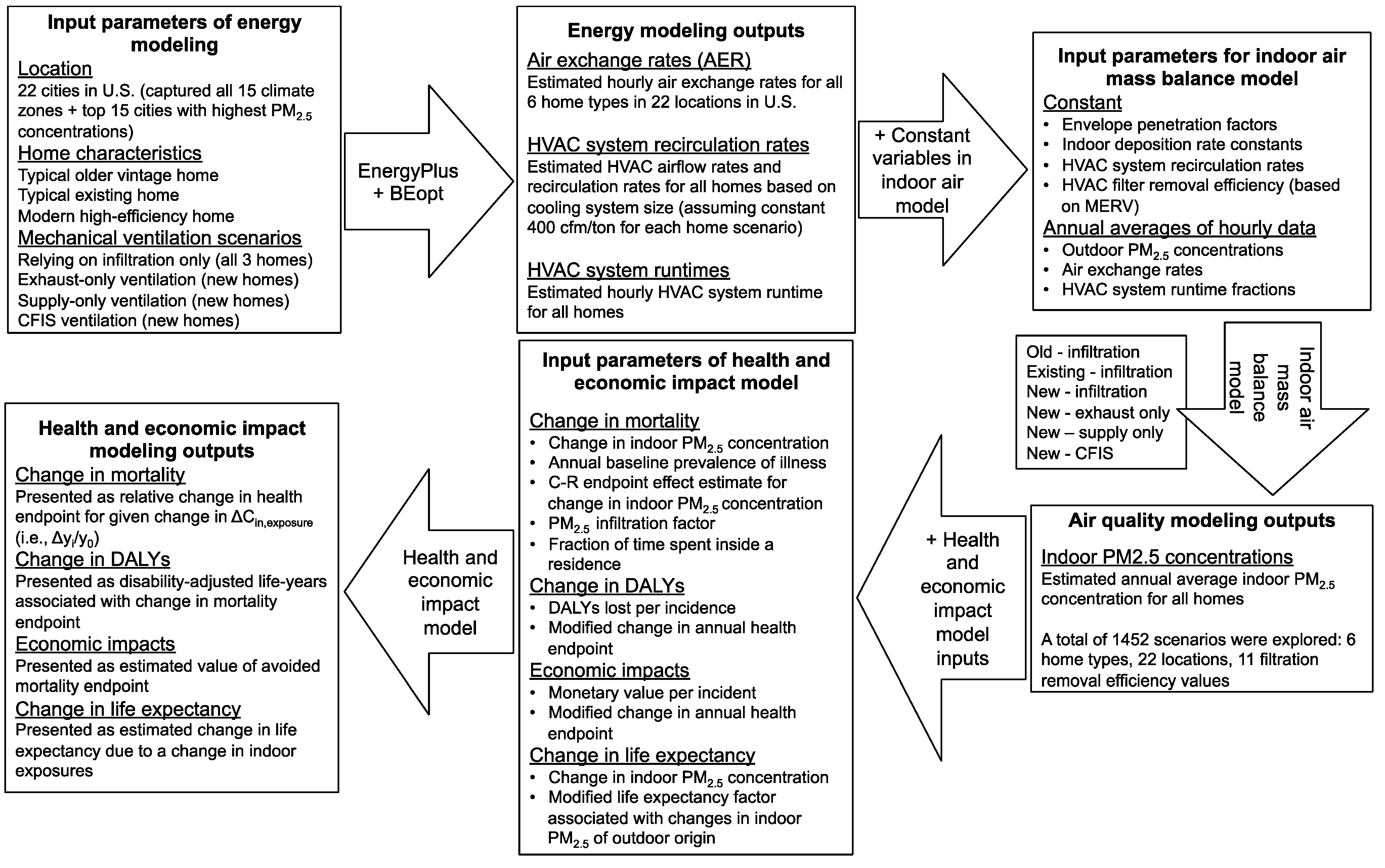
2.1.6. Health and Economic Modeling Inputs Used in This Work

| Modeling outputs | Inputs | Mean | Range | Ref. | |
|---|---|---|---|---|---|
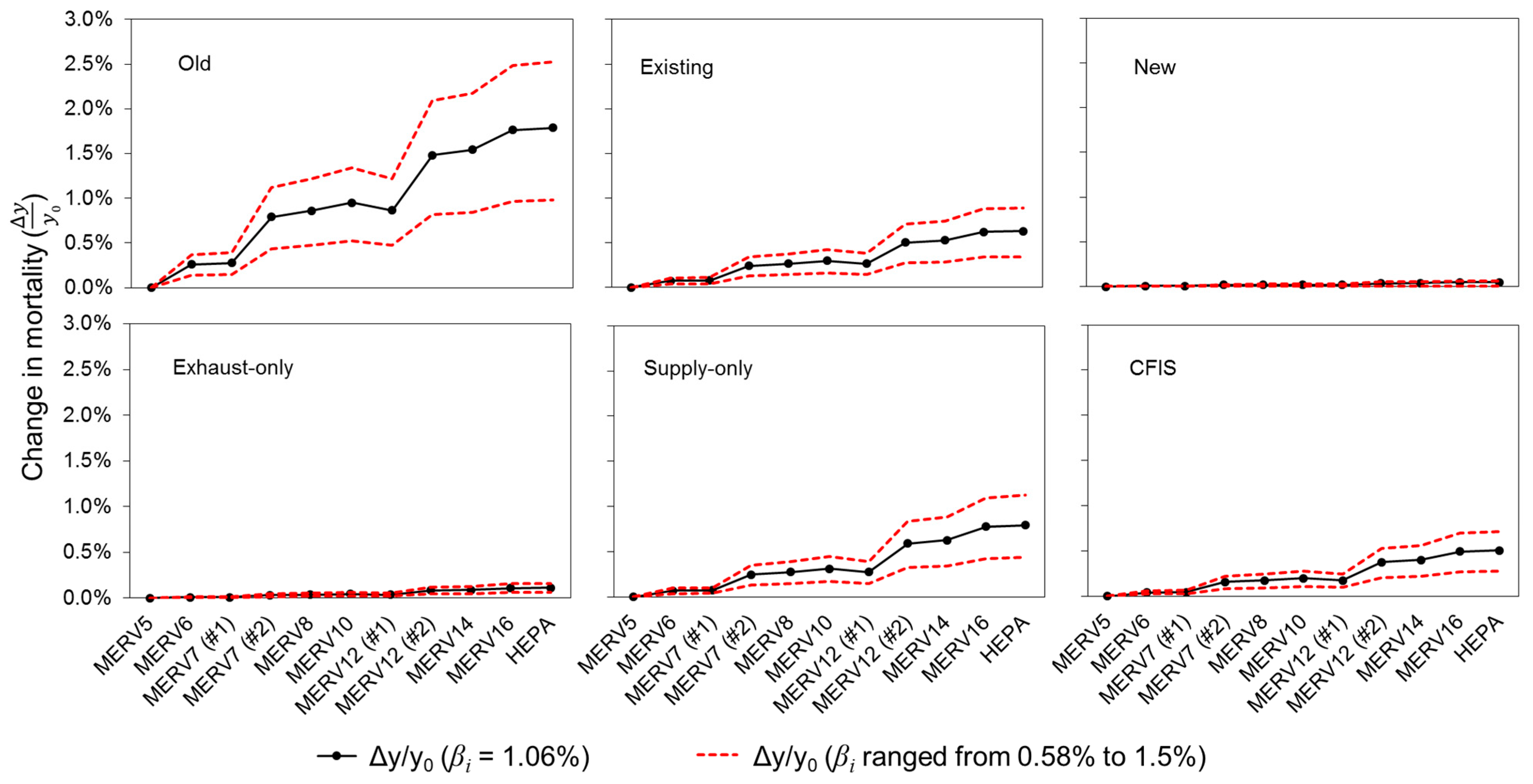
| Change in annual health endpoint (Δyi/y0) | C-R endpoint effect estimate for a change in long-term outdoor PM2.5 concentrations | βi | 1.06% (per µg/m3) | 0.58–1.5% (per µg/m3) | [41], [3], [49] |
| Population-average infiltration factor for PM2.5 | Finf | 0.6 | N/A | [8] | |
| Fraction of time spent inside a residence | Ptime,indoor | 70% | N/A | [7] | |
| Annual baseline prevalence of illness | y0 | 7.38 × 10⁻³ (per person per year) | N/A | [58] | |
| Change in DALYs | DALYs lost per incidence | 1.4 | N/A | [40] | |
| Change in value of avoided mortality endpoint (ΔAi) | Monetary value per incident | $i | $7.2 million | N/A | [59], [60], [61] |
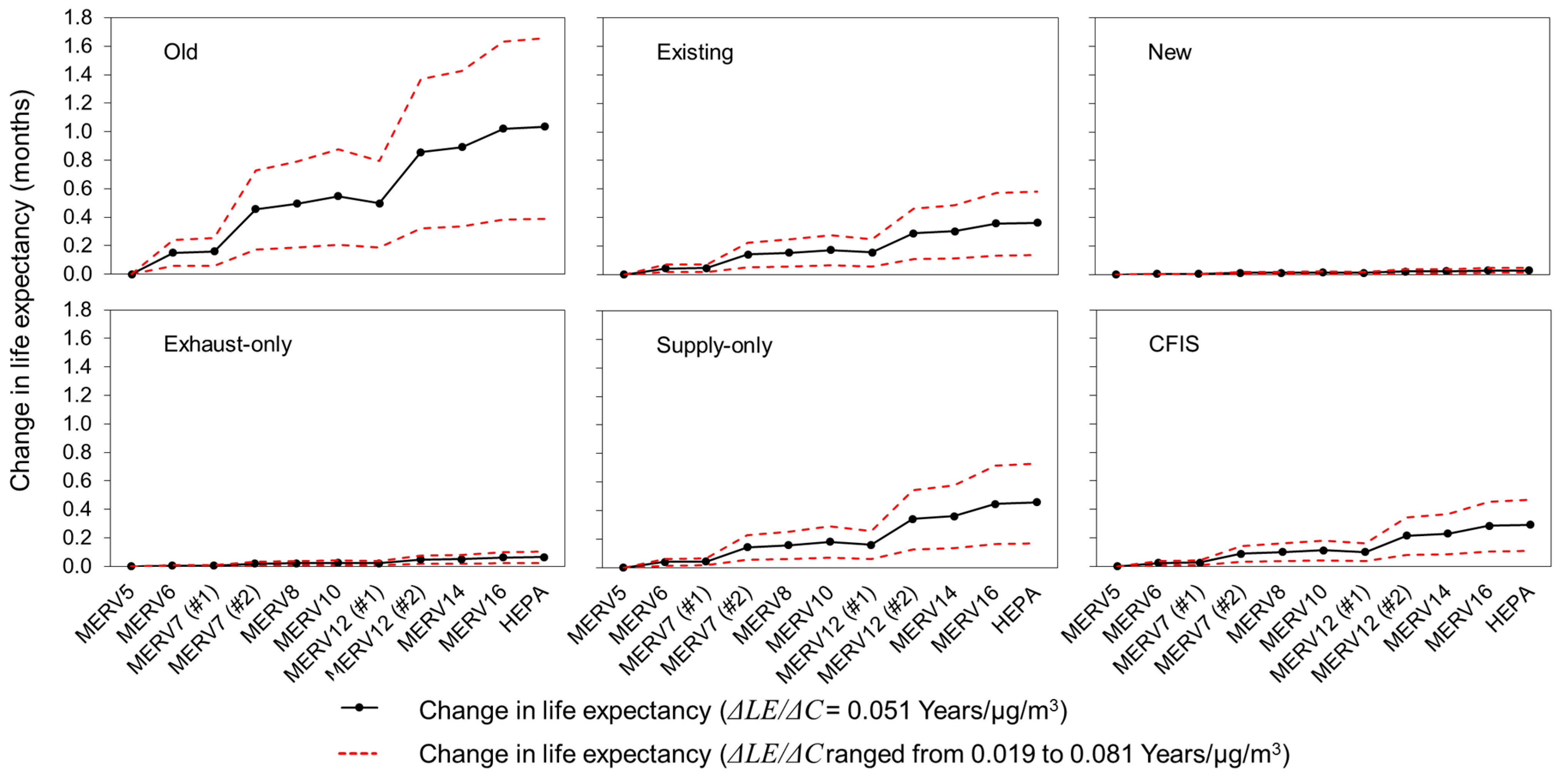
| Change in life expectancy (ΔLE) | Life expectancy factor associated with changes in outdoor PM2.5 concentration | 0.051 (years per µg/m3) | 0.019–0.081 (years per µg/m3) | [1], [62] |
2.2. Modeling Indoor Concentrations of Outdoor PM2.5
2.2.1. Model Home Selection
2.2.2. Mass Balance Modeling
- Finf = PM2.5 infiltration factor for homes without mechanical ventilation (-)
- P = PM2.5 penetration factor of the building envelope (-)
- λinf = air exchange rate due to infiltration (h–1)
- Cout = outdoor PM2.5 concentration (μg/m3)
- kdep = first-order indoor PM2.5 deposition loss rate coefficient (h–1)
- ηHVAC = PM2.5 removal efficiency of the HVAC filter (-)
- λHVAC = HVAC system recirculation rate (HVAC airflow rate divided by volume, h–1)
- f = fractional operation time of the HVAC system (-)
- Constant exhaust-only ventilation;
- Constant supply-only ventilation; and
- Central-fan-integrated-supply (CFIS) with constant exhaust.
- Qfan = minimum mechanical ventilation flow rate (cfm)
- Afloor = floor area (2025 ft2)
- Nbr = number of bedrooms (3)
- Finf,exhaust = PM2.5 infiltration factor for homes with exhaust-only ventilation systems (-)
- λtotal,exhaust = total air exchange rate in new homes with exhaust-only ventilation systems due to a combination of mechanical exhaust and infiltration (h–1)
- fHVAC,exhaust = fractional operation time of the HVAC system in new homes with exhaust-only ventilation systems (-)
- Finf,supply = PM2.5 infiltration factor for homes with supply-only ventilation system (-)
- λfan = air exchange rate due to 50 cfm (85 m3/h) of supply air provided by the mechanical ventilation system (i.e., 0.18/h)
- λtotal,supply = total air exchange rate due to infiltration and ventilation combined (h–1)
- fHVAC,supply= fractional operation time of the HVAC system in new homes with supply-only ventilation system (-)
- ηsupply = PM2.5 removal efficiency of MERV 5 supply ventilation system filter (-)
- Finf,CFIS = PM2.5 infiltration factor for homes with CFIS ventilation systems (-)
- λtotal,CFIS = total air exchange rate due to infiltration and ventilation combined in new homes with CFIS ventilation systems (h–1)
- fHVAC,CFIS = fractional operation time of the HVAC system in new homes with CFIS ventilation systems (-)
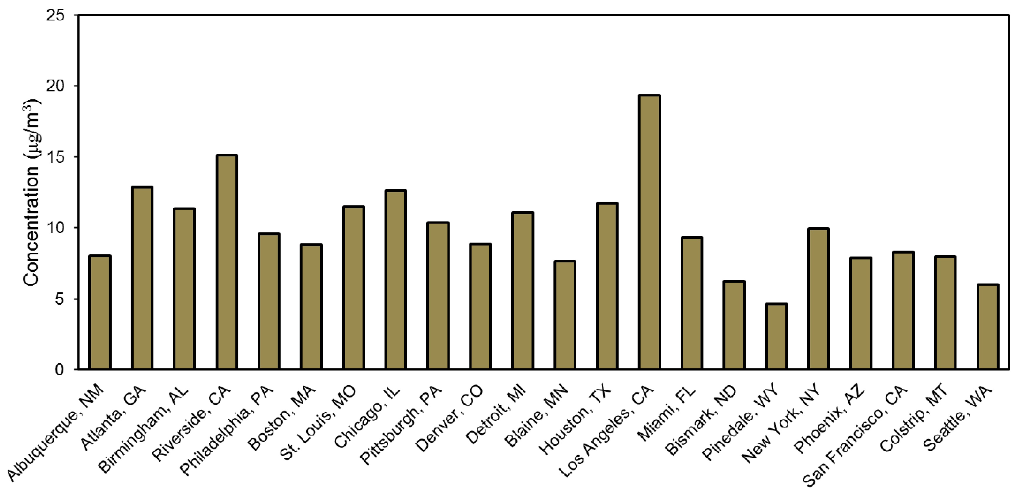
2.2.3. Outdoor PM2.5 Concentrations for Each Geographic Location
| 1. Boston, MA, 5A | 12. Blaine (Minneapolis), MN, 6A |
| 2. New York, NY, 4A | 13. Bismarck, ND, 7A |
| 3. Philadelphia, PA, 4A | 14. Colstrip, MT, 6B |
| 4. Pittsburgh, PA, 5A | 15. Pinedale, WY, 7B |
| 5. Detroit, MI, 5A | 16. Denver, CO, 5B |
| 6. Atlanta, GA, 3A | 17. Albuquerque, NM, 4B |
| 7. Birmingham, AL, 3A | 18. Phoenix, AZ, 2B |
| 8. St. Louis, MO, 4A | 19. Riverside, CA, 3B |
| 9. Chicago, IL, 5A | 20. Los Angeles, CA, 3B |
| 10. Miami, FL, 1A | 21. San Francisco, CA, 3C |
| 11. Houston, TX, 2A | 22. Seattle, WA, 4C |
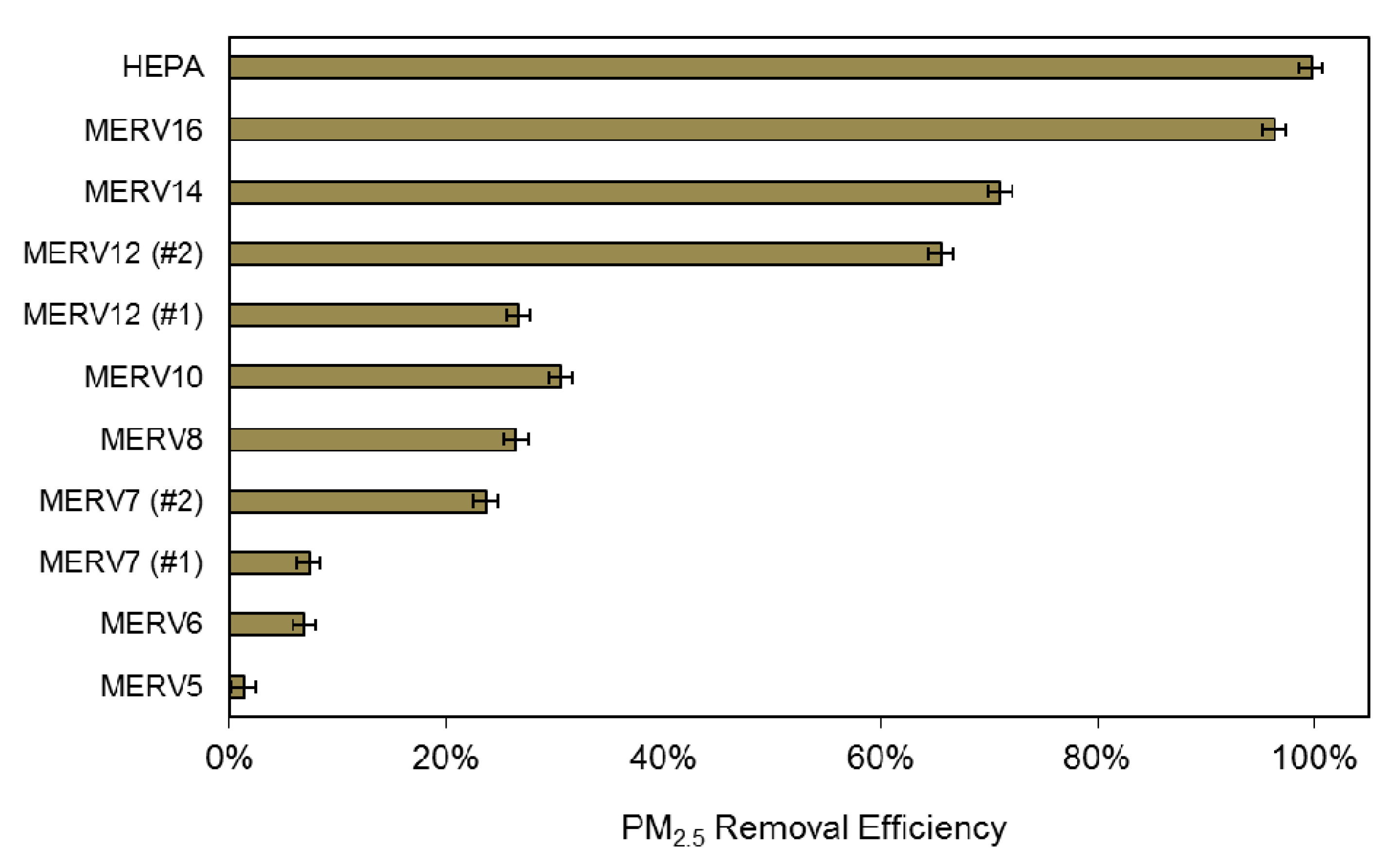
2.2.4. HVAC Filtration Efficiency for PM2.5
2.2.5. PM2.5 Penetration Factors and Deposition Loss Rate Coefficients
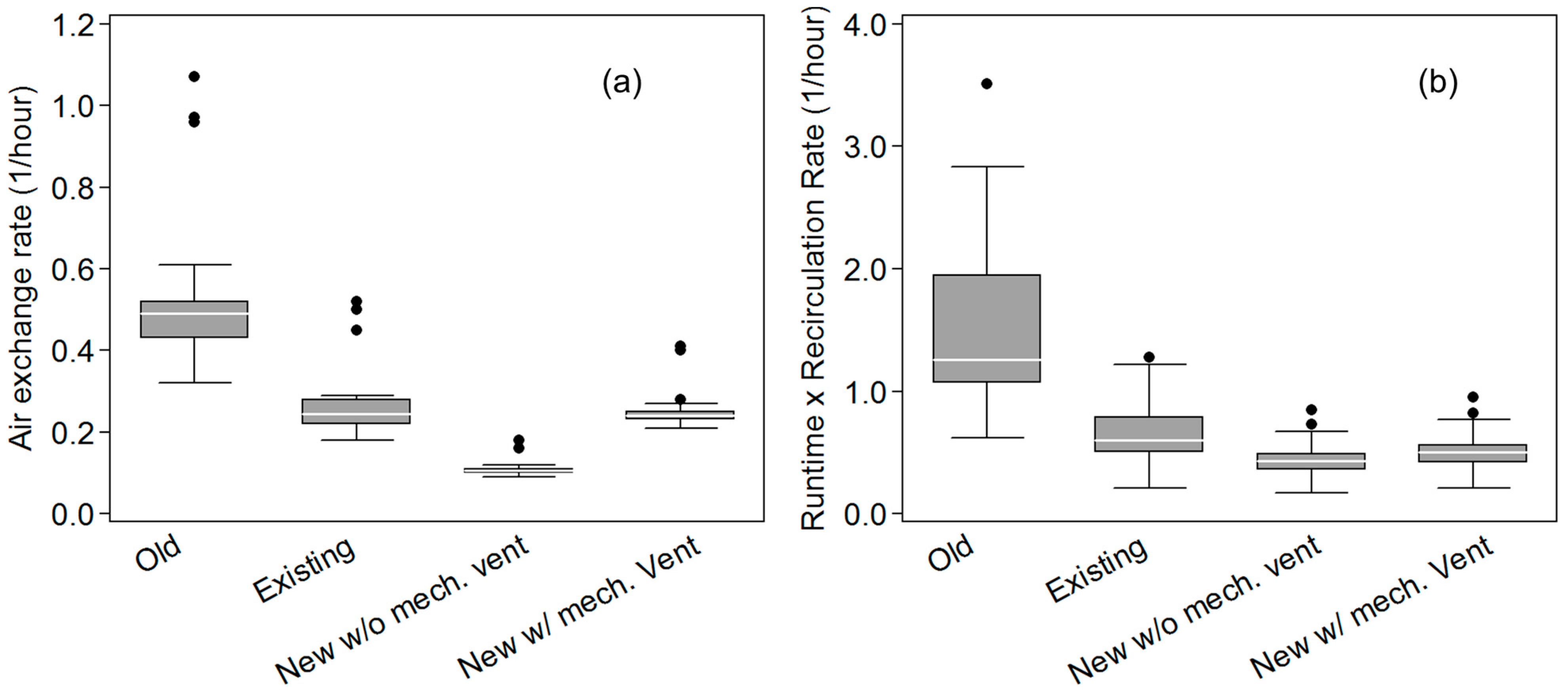
2.2.6. Air Exchange Rates, HVAC Recirculation Rates, and HVAC System Runtimes
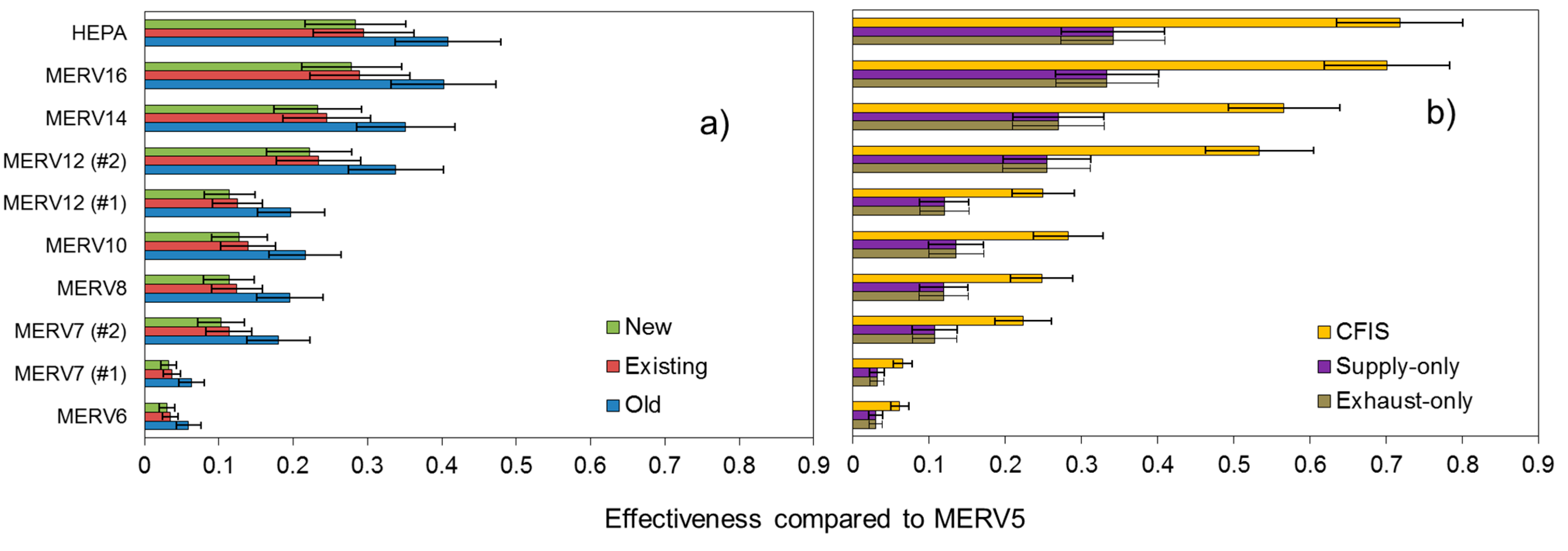
2.2.7. Estimating the Effectiveness of HVAC Filtration for Reducing Indoor PM2.5 of Outdoor Origin
- EMERVj = filtration effectiveness of MERV j filter for PM2.5 of outdoor origin
- Cin,MERVj = annual average estimate of the indoor concentration of PM2.5 when a MERVj filter was installed (μg/m3)
- Cin,MERV5 = annual average estimate of the indoor concentration of PM2.5 when a MERV 5 filter was installed (μg/m3)
3. Results and Discussion
3.1. Annual Average Outdoor PM2.5 Concentrations in Each Location


3.2. Air Exchange Rates, HVAC System Runtimes, and HVAC Recirculation Rates
3.3. PM2.5 Infiltration Factors and Absolute Indoor PM2.5 Concentrations
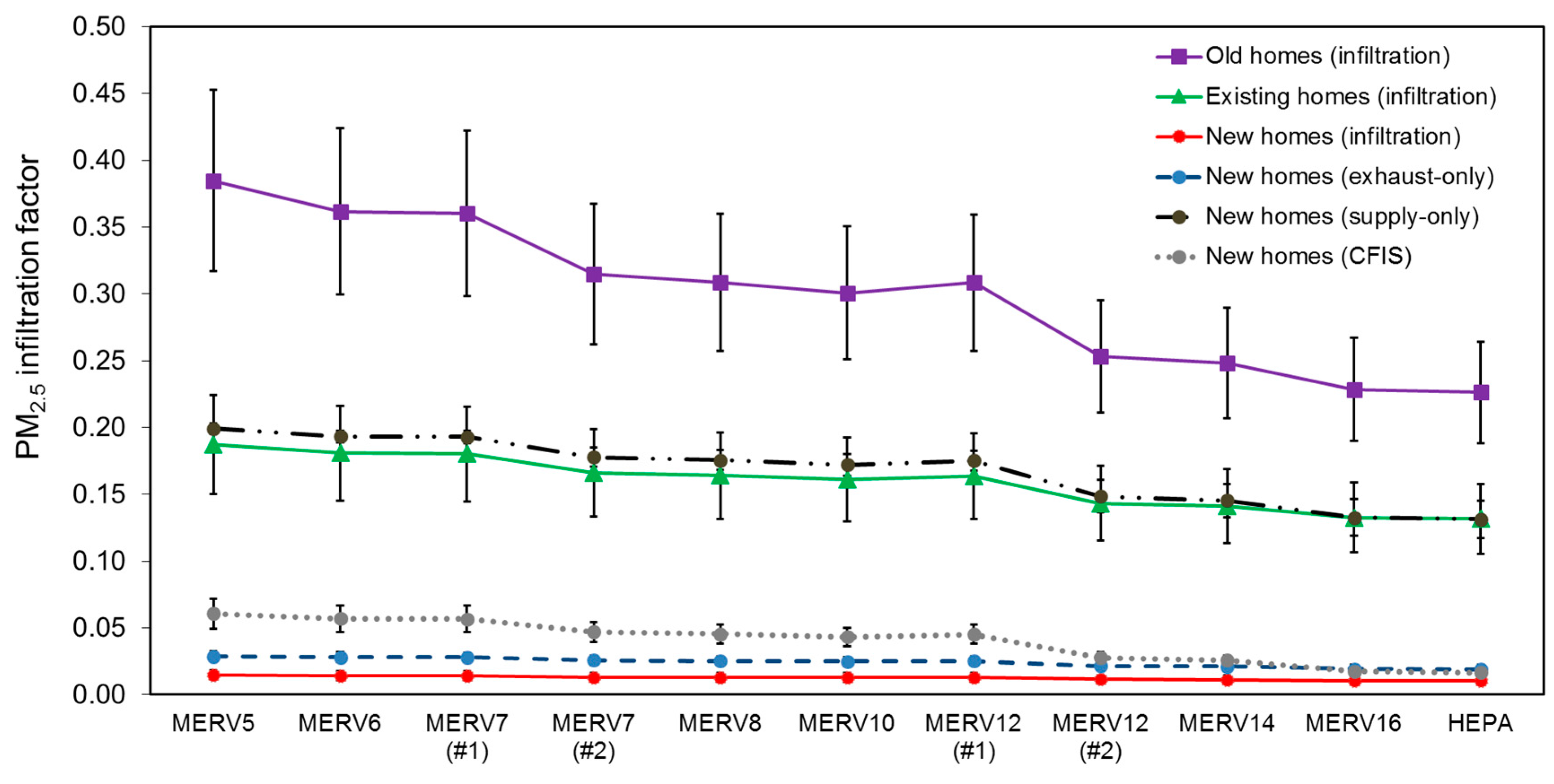

| Old homes | Existing homes | New homes | ||||
|---|---|---|---|---|---|---|
| Infiltration-only | Infiltration-only | Infiltration-only | Exhaust-only | Supply-only | CFIS | |
| MERV 5 | 3.70 (± 0.87) | 1.80 (± 0.44) | 0.15 (± 0.04) | 0.28 (± 0.09) | 1.99 (± 0.65) | 0.58 (± 0.14) |
| MERV 6 | 3.49 (± 0.85) | 1.74 (± 0.43) | 0.14 (± 0.04) | 0.28 (± 0.08) | 1.93 (± 0.64) | 0.55 (± 0.13) |
| MERV 7 (#1) | 3.47 (± 0.85) | 1.73 (± 0.43) | 0.14 (± 0.04) | 0.28 (± 0.08) | 1.93 (± 0.64) | 0.55 (± 0.13) |
| MERV 7 (#2) | 3.04 (± 0.81) | 1.60 (± 0.42) | 0.13 (± 0.04) | 0.26 (± 0.08) | 1.78 (± 0.62) | 0.46 (± 0.11) |
| MERV 8 | 2.99 (± 0.80) | 1.58 (± 0.41) | 0.13 (± 0.04) | 0.25 (± 0.08) | 1.76 (± 0.62) | 0.44 (± 0.11) |
| MERV 10 | 2.91 (± 0.79) | 1.55 (± 0.41) | 0.13 (± 0.04) | 0.25 (± 0.08) | 1.73 (± 0.61) | 0.42 (± 0.11) |
| MERV 12 (#1) | 2.99 (± 0.80) | 1.58 (± 0.41) | 0.13 (± 0.04) | 0.25 (± 0.08) | 1.76 (± 0.62) | 0.44 (± 0.11) |
| MERV 12 (#2) | 2.47 (± 0.75) | 1.38 (± 0.40) | 0.12 (± 0.04) | 0.21 (± 0.08) | 1.50 (± 0.58) | 0.27 (± 0.09) |
| MERV 14 | 2.42 (± 0.75) | 1.36 (± 0.39) | 0.11 (± 0.04) | 0.21 (± 0.08) | 1.47 (± 0.57) | 0.26 (± 0.08) |
| MERV 16 | 2.24 (± 0.73) | 1.29 (± 0.39) | 0.11 (± 0.04) | 0.19 (± 0.07) | 1.35 (± 0.55) | 0.18 (± 0.07) |
| HEPA | 2.21 (± 0.72) | 1.28 (± 0.39) | 0.11 (± 0.04) | 0.19 (± 0.07) | 1.33 (± 0.55) | 0.17 (± 0.07) |
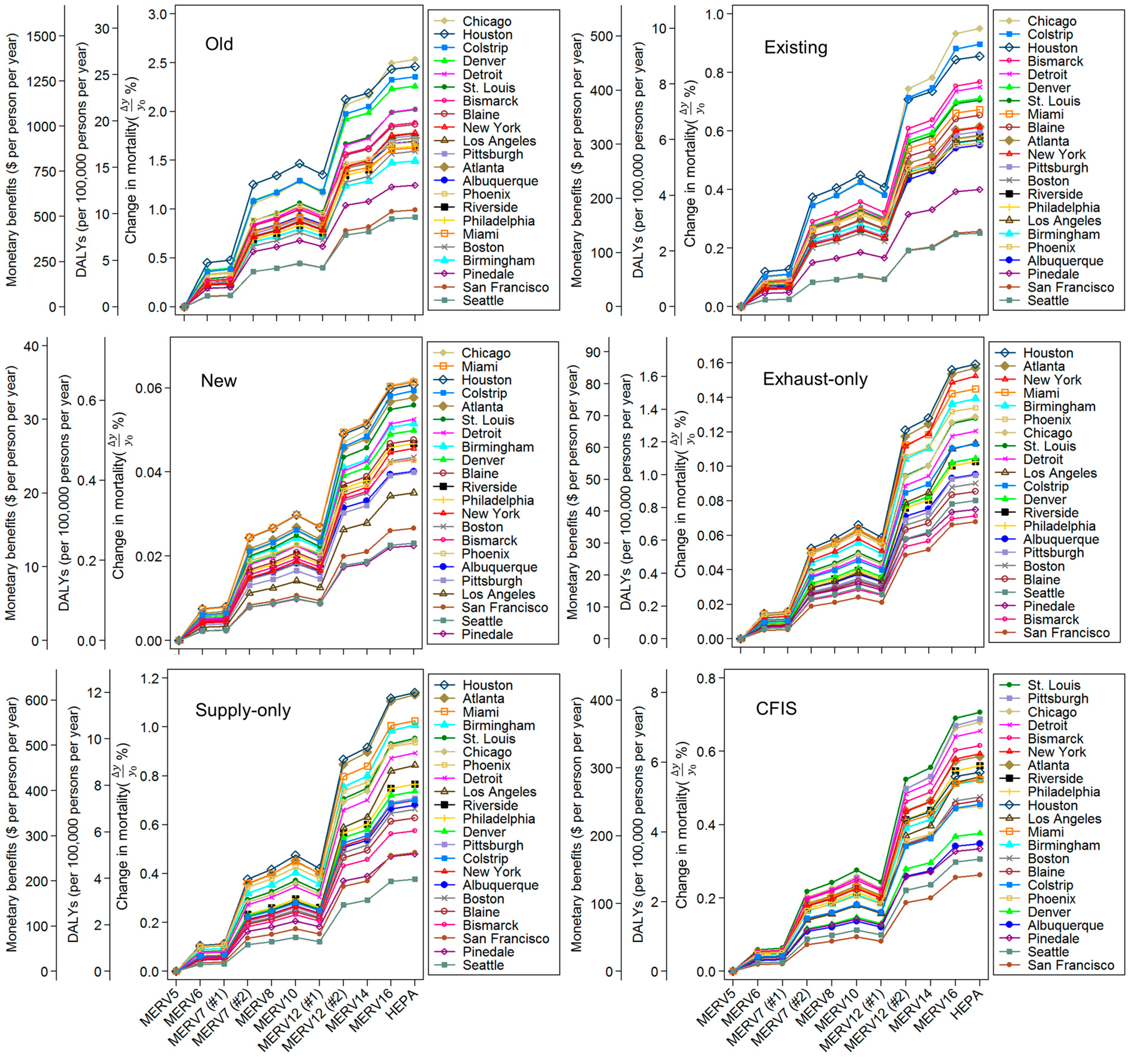
3.4. The Impact of HVAC Filters on Premature Mortality Associated with Indoor PM2.5 of Outdoor Origin

3.5. Impact of Home Location and Outdoor PM2.5 Concentrations on Premature Mortality, DALYs, and Monetized Benefits
3.6. Impact of HVAC Filtration on Life Expectancy
3.7. Limitations
4. Conclusions
Acknowledgments
Author Contributions
Conflicts of Interest
References and Notes
- Pope, C.A.; Ezzati, M.; Dockery, D.W. Fine-Particulate Air Pollution and Life Expectancy in the United States. N. Engl. J. Med. 2009, 360, 376–386. [Google Scholar] [CrossRef] [PubMed]
- Pope, C.A., III; Dockery, D.W. Health Effects of Fine Particulate Air Pollution: Lines that Connect. J. Air Waste Manag. Assoc. 2006, 56, 709–742. [Google Scholar] [CrossRef] [PubMed]
- Pope, C.A., III; Burnett, R.T.; Thun, M.J.; Calle, E.E.; Krewski, D.; Ito, K.; Thurston, G.D. Lung cancer, cardiopulmonary mortality, and long-term exposure to fine particulate air pollution. Jama 2002, 287, 1132–1141. [Google Scholar] [CrossRef] [PubMed]
- Miller, K.A.; Siscovick, D.S.; Sheppard, L.; Shepherd, K.; Sullivan, J.H.; Anderson, G.L.; Kaufman, J.D. Long-term exposure to air pollution and incidence of cardiovascular events in women. N. Engl. J. Med. 2007, 356, 447–458. [Google Scholar] [CrossRef] [PubMed]
- Dockery, D.W.; Pope, C.A.; Xu, X.; Spengler, J.D.; Ware, J.H.; Fay, M.E.; Ferris, B.G.; Speizer, F.E. An Association between Air Pollution and Mortality in Six U.S. Cities. N. Engl. J. Med. 1993, 329, 1753–1759. [Google Scholar] [CrossRef] [PubMed]
- Brook, R.D.; Rajagopalan, S.; Pope, C.A.; Brook, J.R.; Bhatnagar, A.; Diez-Roux, A.V.; Holguin, F.; Hong, Y.; Luepker, R.V.; Mittleman, M.A.; et al. Particulate matter air pollution and cardiovascular disease an update to the scientific statement from the American Heart Association. Circulation 2010, 121, 2331–2378. [Google Scholar] [CrossRef] [PubMed]
- Klepeis, N.E.; Nelson, W.C.; Ott, W.R.; Robinson, J.P.; Tsang, A.M.; Switzer, P.; Behar, J.V.; Hern, S.C.; Engelmann, W.H. The National Human Activity Pattern Survey (NHAPS): A resource for assessing exposure to environmental pollutants. J. Expo. Anal. Environ. Epidemiol. 2001, 11, 231–252. [Google Scholar] [CrossRef] [PubMed]
- Chen, C.; Zhao, B. Review of relationship between indoor and outdoor particles: I/O ratio, infiltration factor and penetration factor. Atmos. Environ. 2011, 45, 275–288. [Google Scholar] [CrossRef]
- Kearney, J.; Wallace, L.; MacNeill, M.; Héroux, M.-E.; Kindzierski, W.; Wheeler, A. Residential infiltration of fine and ultrafine particles in Edmonton. Atmos. Environ. 2014, 94, 793–805. [Google Scholar] [CrossRef]
- Wallace, L.; Williams, R. Use of Personal-Indoor-Outdoor Sulfur Concentrations to Estimate the Infiltration Factor and Outdoor Exposure Factor for Individual Homes and Persons. Environ. Sci. Technol. 2005, 39, 1707–1714. [Google Scholar] [CrossRef] [PubMed]
- Meng, Q.Y.; Spector, D.; Colome, S.; Turpin, B. Determinants of indoor and personal exposure to PM2.5 of indoor and outdoor origin during the RIOPA study. Atmos. Environ. 2009, 43, 5750–5758. [Google Scholar] [CrossRef] [PubMed]
- Allen, R.; Wallace, L.; Larson, T.; Sheppard, L.; Liu, L.J. Estimated Hourly Personal Exposures to Ambient and Nonambient Particulate Matter Among Sensitive Populations in Seattle, Washington. J. Air Waste Manag. Assoc. 2004, 54, 1197–1211. [Google Scholar] [CrossRef] [PubMed]
- Baxter, L.K.; Burke, J.; Lunden, M.; Turpin, B.J.; Rich, D.Q.; Thevenet-Morrison, K.; Hodas, N.; Özkaynak, H. Influence of human activity patterns, particle composition, and residential air exchange rates on modeled distributions of PM2.5 exposure compared with central-site monitoring data. J. Expo. Sci. Environ. Epidemiol. 2013, 23, 241–247. [Google Scholar] [CrossRef] [PubMed]
- Baxter, L.K.; Clougherty, J.E.; Paciorek, C.J.; Wright, R.J.; Levy, J.I. Predicting residential indoor concentrations of nitrogen dioxide, fine particulate matter, and elemental carbon using questionnaire and geographic information system based data. Atmos. Environ. 2007, 41, 6561–6571. [Google Scholar] [CrossRef] [PubMed]
- Baxter, L.K.; Franklin, M.; Özkaynak, H.; Schultz, B.D.; Neas, L.M. The use of improved exposure factors in the interpretation of fine particulate matter epidemiological results. Air Qual. Atmosphere Health 2011, 6, 195–204. [Google Scholar] [CrossRef]
- Allen, R.W.; Adar, S.D.; Avol, E.; Cohen, M.; Curl, C.L.; Larson, T.; Liu, L.J.; Sheppard, L.; Kaufman, J.D. Modeling the Residential Infiltration of Outdoor PM2.5 in the Multi-Ethnic Study of Atherosclerosis and Air Pollution (MESA Air). Environ. Health Perspect. 2012, 120, 824–830. [Google Scholar] [CrossRef] [PubMed]
- Hodas, N.; Meng, Q.; Lunden, M.M.; Rich, D.Q.; Ozkaynak, H.; Baxter, L.K.; Zhang, Q.; Turpin, B.J. Variability in the fraction of ambient fine particulate matter found indoors and observed heterogeneity in health effect estimates. J. Expo. Sci. Environ. Epidemiol. 2012, 22, 448–454. [Google Scholar] [CrossRef] [PubMed]
- Hodas, N.; Turpin, B.J.; Lunden, M.M.; Baxter, L.K.; Özkaynak, H.; Burke, J.; Ohman-Strickland, P.; Thevenet-Morrison, K.; Kostis, J.B.; Rich, D.Q. Refined ambient PM2.5 exposure surrogates and the risk of myocardial infarction. J. Expo. Sci. Environ. Epidemiol. 2013, 23, 573–580. [Google Scholar] [CrossRef] [PubMed]
- MacNeill, M.; Wallace, L.; Kearney, J.; Allen, R.W.; Van Ryswyk, K.; Judek, S.; Xu, X.; Wheeler, A. Factors influencing variability in the infiltration of PM2.5 mass and its components. Atmos. Environ. 2012, 61, 518–532. [Google Scholar] [CrossRef]
- MacNeill, M.; Kearney, J.; Wallace, L.; Gibson, M.; Héroux, M.E.; Kuchta, J.; Guernsey, J.R.; Wheeler, A.J. Quantifying the contribution of ambient and indoor-generated fine particles to indoor air in residential environments. Indoor Air 2014, 24, 362–375. [Google Scholar] [CrossRef] [PubMed]
- Meng, Q.Y.; Turpin, B.J.; Korn, L.; Weisel, C.P.; Morandi, M.; Colome, S.; Zhang, J.J.; Stock, T.; Spektor, D.; Winer, A.; Zhang, L.; Lee, J.H.; Giovanetti, R.; Cui, W.; Kwon, J.; Alimokhtari, S.; Shendell, D.; Jones, J.; Farrar, C.; Maberti, S. Influence of ambient (outdoor) sources on residential indoor and personal PM2.5 concentrations: analyses of RIOPA data. J. Expo. Anal. Environ. Epidemiol. 2005, 15, 17–28. [Google Scholar] [CrossRef] [PubMed]
- Ji, W.; Zhao, B. Estimating Mortality Derived from Indoor Exposure to Particles of Outdoor Origin. PLoS ONE 2015, 10, e0124238. [Google Scholar] [CrossRef] [PubMed]
- Bräuner, E.V.; Forchhammer, L.; Møller, P.; Barregard, L.; Gunnarsen, L.; Afshari, A.; Wåhlin, P.; Glasius, M.; Dragsted, L.O.; Basu, S.; Raaschou-Nielsen, O.; Loft, S. Indoor particles affect vascular function in the aged: an air filtration-based intervention study. Am. J. Respir. Crit. Care Med. 2008, 177, 419–425. [Google Scholar] [CrossRef] [PubMed]
- Brown, K.W.; Minegishi, T.; Allen, J.G.; McCarthy, J.F.; Spengler, J.D.; MacIntosh, D.L. Reducing patients’ exposures to asthma and allergy triggers in their homes: an evaluation of effectiveness of grades of forced air ventilation filters. J. Asthma Off. J. Assn. Care Asthma 2014, 51, 585–594. [Google Scholar] [CrossRef] [PubMed]
- Burroughs, H.E.B.; Kinzer, K.E. Improved filtration in residential environments. Ashrae J. 1998, 40, 47–51. [Google Scholar]
- Fugler, D.; Bowser, D.; Kwan, W. The effects of improved residential furnace filtration on airborne particles. ASHRAE Trans. 2000, 106, 317–326. [Google Scholar]
- Lin, L.-Y.; Chen, H.-W.; Su, T.-L.; Hong, G.-B.; Huang, L.-C.; Chuang, K.-J. The effects of indoor particle exposure on blood pressure and heart rate among young adults: An air filtration-based intervention study. Atmos. Environ. 2011, 45, 5540–5544. [Google Scholar] [CrossRef]
- Macintosh, D.L.; Minegishi, T.; Kaufman, M.; Baker, B.J.; Allen, J.G.; Levy, J.I.; Myatt, T.A. The benefits of whole-house in-duct air cleaning in reducing exposures to fine particulate matter of outdoor origin: a modeling analysis. J. Expo. Sci. Environ. Epidemiol. 2010, 20, 213–224. [Google Scholar] [CrossRef] [PubMed]
- Stephens, B.; Siegel, J.; Novoselac, A. Energy Implications of Filtration in Residential and Light-Commercial Construction; ASHRAE Research Project-1299; American Society of Heating, Refrigerating, and Air-Conditioning Engineers, Inc.: Orlando, FL, USA, 2010. [Google Scholar]
- Stephens, B.; Siegel, J.A. Ultrafine particle removal by residential heating, ventilating, and air-conditioning filters. Indoor Air 2013, 23, 488–497. [Google Scholar] [CrossRef] [PubMed]
- Riley, W.J.; McKone, T.E.; Lai, A.C.K.; Nazaroff, W.W. Indoor Particulate Matter of Outdoor Origin: Importance of Size-Dependent Removal Mechanisms. Environ. Sci. Technol. 2002, 36, 200–207. [Google Scholar] [CrossRef] [PubMed]
- Fisk, W.J. Health benefits of particle filtration. Indoor Air 2013, 23, 357–368. [Google Scholar] [CrossRef] [PubMed]
- Montgomery, J.F.; Reynolds, C.C.O.; Rogak, S.N.; Green, S.I. Financial implications of modifications to building filtration systems. Bldg. Environ. 2015, 85, 17–28. [Google Scholar] [CrossRef]
- Bekö, G.; Clausen, G.; Weschler, C.J. Is the use of particle air filtration justified? Costs and benefits of filtration with regard to health effects, building cleaning and occupant productivity. Bldg. Environ. 2008, 43, 1647–1657. [Google Scholar] [CrossRef]
- Chan, W.R.; Parthasarathy, S.; Fisk, W.J.; McKone, T.E. Estimated effect of ventilation and filtration on chronic health risks in U.S. offices, schools, and retail stores. Indoor Air 2015. [Google Scholar] [CrossRef] [PubMed]
- Zuraimi, M.S.; Tan, Z. Impact of residential building regulations on reducing indoor exposures to outdoor PM2.5 in Toronto. Bldg. Environ. 2015, 89, 336–344. [Google Scholar] [CrossRef]
- Standard, A. Standard 52.2-2007–Method of testing general ventilation air-cleaning devices for removal efficiency by particle size (ANSI/ASHRAE Approved). Am. Soc. Heat. Refrig. Air-Cond. Eng. 2007. [Google Scholar]
- ASHRAE. Standard 62.2: Ventilation and Acceptable Indoor Air Quality in Low-Rise Residential Buildings; American Society of Heating, Refrigerating and Air-Conditioning Engineers, Inc.: Orlando, FL, USA, 2013. [Google Scholar]
- Stieb, D.M.; Judek, S.; Brand, K.; Burnett, R.T.; Shin, H.H. Approximations for Estimating Change in Life Expectancy Attributable to Air Pollution in Relation to Multiple Causes of Death Using a Cause Modified Life Table. Risk Anal. 2015. [Google Scholar] [CrossRef] [PubMed]
- Logue, J.M.; Price, P.N.; Sherman, M.H.; Singer, B.C. A Method to Estimate the Chronic Health Impact of Air Pollutants in U.S. Residences. Environ. Health Perspect. 2012, 120, 216–222. [Google Scholar] [CrossRef] [PubMed]
- US EPA. The Benefits and Costs of the Clean Air Act from 1990 to 2020; U.S. Environmental Protection Agency Office of Air and Radiation: Washington, DC, USA, 2011.
- Pope, C.A.; Thun, M.J.; Namboodiri, M.M.; Dockery, D.W.; Evans, J.S.; Speizer, F.E.; Heath, C.W. Particulate Air Pollution as a Predictor of Mortality in a Prospective Study of U.S. Adults. Am. J. Respir. Crit. Care Med. 1995, 151, 669–674. [Google Scholar] [CrossRef] [PubMed]
- IEc. Health and Welfare Benefits Analyses to Support the Second Section 812 Benefit-Cost Analysis of the Clean Air Act; Industrial Economics, Inc.: Cambridge, MA, UK, 2011. [Google Scholar]
- Murray, C.J.; Lopez, A.D. Alternative projections of mortality and disability by cause 1990–2020: Global Burden of Disease Study. The Lancet 1997, 349, 1498–1504. [Google Scholar] [CrossRef]
- Lvovsky, K.; Hughes, G.; Maddison, D.; Ostro, B.; Pearce, D. Environmental Costs of Fossil Fuels: A Rapid Assessment Method with Application to Six Cities; Working Paper, Environment Department Papers 78; World Bank: Washington, DC, USA, 2000. [Google Scholar]
- Huijbregts, M.A.J.; Rombouts, L.J.A.; Ragas, A.M.J.; van de Meent, D. Human-toxicological effect and damage factors of carcinogenic and noncarcinogenic chemicals for life cycle impact assessment. Integr. Environ. Assess. Manag. 2005, 1, 181–244. [Google Scholar] [CrossRef] [PubMed]
- World Health Organization. Global Health Risks: Mortality and Burden of Disease Attributable to Selected Major Risks; World Health Organization, 2009.
- Gao, T.; Wang, X.C.; Chen, R.; Ngo, H.H.; Guo, W. Disability adjusted life year (DALY): A useful tool for quantitative assessment of environmental pollution. Sci. Total Environ. 2015, 511, 268–287. [Google Scholar] [CrossRef] [PubMed]
- Laden, F.; Schwartz, J.; Speizer, F.E.; Dockery, D.W. Reduction in Fine Particulate Air Pollution and Mortality: Extended Follow-up of the Harvard Six Cities Study. Amer. J. Respir. Crit. Care Med. 2006, 173, 667–672. [Google Scholar] [CrossRef] [PubMed]
- Roman, H.A.; Walker, K.D.; Walsh, T.L.; Conner, L.; Richmond, H.M.; Hubbell, B.J.; Kinney, P.L. Expert Judgment Assessment of the Mortality Impact of Changes in Ambient Fine Particulate Matter in the U.S. Environ. Sci. Technol. 2008, 42, 2268–2274. [Google Scholar] [CrossRef] [PubMed]
- Zeger, S.L.; Dominici, F.; McDermott, A.; Samet, J.M. Mortality in the Medicare population and chronic exposure to fine particulate air pollution in urban centers (2000–2005). Environ. Health Perspect. 2008, 116, 1614–1619. [Google Scholar] [CrossRef] [PubMed]
- Eftim, S.E.; Samet, J.M.; Janes, H.; McDermott, A.; Dominici, F. Fine particulate matter and mortality: A comparison of the six cities and American Cancer Society cohorts with a medicare cohort. Epidemiol. Camb. Mass 2008, 19, 209–216. [Google Scholar] [CrossRef] [PubMed]
- Puett, R.C.; Schwartz, J.; Hart, J.E.; Yanosky, J.D.; Speizer, F.E.; Suh, H.; Paciorek, C.J.; Neas, L.M.; Laden, F. Chronic particulate exposure, mortality, and coronary heart disease in the nurses’ health study. Am. J. Epidemiol. 2008, 168, 1161–1168. [Google Scholar] [CrossRef] [PubMed]
- Aldred, J.R.; Darling, E.; Morrison, G.; Siegel, J.; Corsi, R. Benefit-Cost analysis of commercially available activated carbon filters for indoor ozone removal in single-family homes. Indoor Air 2015. [Google Scholar] [CrossRef] [PubMed]
- Chen, C.; Zhao, B.; Weschler, C.J. Indoor exposure to “outdoor PM10.”. Epidemiology 2012, 23, 870–878. [Google Scholar] [CrossRef] [PubMed]
- Chen, C.; Zhao, B.; Weschler, C.J. Assessing the influence of indoor exposure to “Outdoor Ozone” on the relationship between ozone and short-term mortality in U.S. communities. Environ. Health Perspect. 2012, 120, 235–240. [Google Scholar] [CrossRef] [PubMed]
- Rosner, B.; Willett, W.C.; Spiegelman, D. Correction of logistic regression relative risk estimates and confidence intervals for systematic within-person measurement error. Stat. Med. 1989, 8, 1051–1069. [Google Scholar] [CrossRef] [PubMed]
- NVSS. National Vital Statistics System Homepage. Available online: http://www.cdc.gov/nchs/nvss.htm (accessed on 31 March 2015).
- US EPA. Mortality Risk Valuation | Guidelines | Publications | NCEE | US EPA. Available online: http://yosemite.epa.gov/EE%5Cepa%5Ceed.nsf/webpages/MortalityRiskValuation.html#process (accessed on 16 April 2015).
- Robinson, L.A. Policy monitor: How us government agencies value mortality risk reductions. Rev. Environ. Econ. Policy 2007, 1, 283–299. [Google Scholar] [CrossRef]
- Trottenberg, P. Treatment of the Value of Preventing Fatalities and Injuries in Preparing Economic Analysis—2011 Revision; US Department of Transportation: Washington, DC, USA, 2011.
- Correia, A.W.; Pope, C.A., III; Dockery, D.W.; Wang, Y.; Ezzati, M.; Dominici, F. The effect of air pollution control on life expectancy in the United States: an analysis of 545 US counties for the period 2000 to 2007. Epidemiol. Camb. Mass 2013, 24, 23. [Google Scholar] [CrossRef] [PubMed]
- El Orch, Z.; Stephens, B.; Waring, M.S. Predictions and determinants of size-resolved particle infiltration factors in single-family homes in the U.S. Bldg. Environ. 2014, 74, 106–118. [Google Scholar] [CrossRef]
- Azimi, P.; Zhao, D.; Stephens, B. Modeling the Impact of Residential HVAC Filtration on Indoor Particles of Outdoor Origin; ASHRAE Research Project 1691-RP; American Society of Heating, Refrigerating, and Air-Conditioning Engineers, Inc.: Orlando, FL, USA, 2015. [Google Scholar]
- IECC. International Energy Conservation Code; International Code Council, Inc.: Country Club Hills, IL, USA, 2012. [Google Scholar]
- Walker, I.S.; Sherman, M.H. Effect of ventilation strategies on residential ozone levels. Bldg. Environ. 2013, 59, 456–465. [Google Scholar] [CrossRef]
- US EPA. Integrated Science Assessment for Particulate Matter; National Center for Environmental Assessment: Research Triangle Park, NC, USA, 2009.
- US EPA. AQS Data for Downloading, TTN AIRS AQS. Available online: http://www.epa.gov/ttn/airs/airsaqs/detaildata/downloadaqsdata.htm (accessed on 11 December 2014).
- Azimi, P.; Zhao, D.; Stephens, B. Estimates of HVAC filtration efficiency for fine and ultrafine particles of outdoor origin. Atmos. Environ. 2014, 98, 337–346. [Google Scholar] [CrossRef]
- Stephens, B. Building design and operational choices that impact indoor exposures to outdoor particulate matter inside residences. Sci. Technol. Built Environ. 2015, 21, 3–13. [Google Scholar] [CrossRef]
- Stephens, B.; Siegel, J.A. Penetration of ambient submicron particles into single-family residences and associations with building characteristics. Indoor Air 2012, 22, 501–513. [Google Scholar] [CrossRef] [PubMed]
- Lachenmyer, C. Urban measurements of outdoor-indoor PM2.5 concentrations and personal exposure in the deep south. part I. pilot study of mass concentrations for nonsmoking subjects. Aerosol Sci. Technol. 2000, 32, 34–51. [Google Scholar] [CrossRef]
- Williams, R.; Suggs, J.; Rea, A.; Sheldon, L.; Rodes, C.; Thornburg, J. The research triangle park particulate matter panel study: Modeling ambient source contribution to personal and residential PM mass concentrations. Atmos. Environ. 2003, 37, 5365–5378. [Google Scholar] [CrossRef]
- Wallace, L.; Kindzierski, W.; Kearney, J.; MacNeill, M.; Héroux, M.-È.; Wheeler, A.J. Fine and ultrafine particle decay rates in multiple homes. Environ. Sci. Technol. 2013, 47, 12929–12937. [Google Scholar] [CrossRef] [PubMed]
- Clark, N.A.; Allen, R.W.; Hystad, P.; Wallace, L.; Dell, S.D.; Foty, R.; Dabek-Zlotorzynska, E.; Evans, G.; Wheeler, A.J. Exploring variation and predictors of residential fine particulate matter infiltration. Int. J. Environ. Res. Public Health 2010, 7, 3211–3224. [Google Scholar] [CrossRef] [PubMed]
- Stephens, B.; Siegel, J.A.; Novoselac, A. Energy implications of filtration in residential and light-commercial buildings (RP-1299). ASHRAE Trans. 2010, 116, 346–357. [Google Scholar]
- Stephens, B.; Novoselac, A.; Siegel, J.A. The effects of filtration on pressure drop and energy consumption in residential HVAC systems. Hvac&R Res. 2010, 16, 273–294. [Google Scholar]
- Walker, I.S.; Dickerhoff, D.J.; Faulkner, D.; Turner, W.J.N. Energy Implications of In-Line Filtration in California; Lawrence Berkeley National Laboratory: Berkeley, CA, USA, 2012. [Google Scholar]
- Azimi, P.; Stephens, B. HVAC filtration for controlling infectious airborne disease transmission in indoor environments: Predicting risk reductions and operational costs. Bldg. Environ. 2013, 70, 150–160. [Google Scholar] [CrossRef]
© 2015 by the authors; licensee MDPI, Basel, Switzerland. This article is an open access article distributed under the terms and conditions of the Creative Commons Attribution license (http://creativecommons.org/licenses/by/4.0/).
Share and Cite
Zhao, D.; Azimi, P.; Stephens, B. Evaluating the Long-Term Health and Economic Impacts of Central Residential Air Filtration for Reducing Premature Mortality Associated with Indoor Fine Particulate Matter (PM2.5) of Outdoor Origin. Int. J. Environ. Res. Public Health 2015, 12, 8448-8479. https://doi.org/10.3390/ijerph120708448
Zhao D, Azimi P, Stephens B. Evaluating the Long-Term Health and Economic Impacts of Central Residential Air Filtration for Reducing Premature Mortality Associated with Indoor Fine Particulate Matter (PM2.5) of Outdoor Origin. International Journal of Environmental Research and Public Health. 2015; 12(7):8448-8479. https://doi.org/10.3390/ijerph120708448
Chicago/Turabian StyleZhao, Dan, Parham Azimi, and Brent Stephens. 2015. "Evaluating the Long-Term Health and Economic Impacts of Central Residential Air Filtration for Reducing Premature Mortality Associated with Indoor Fine Particulate Matter (PM2.5) of Outdoor Origin" International Journal of Environmental Research and Public Health 12, no. 7: 8448-8479. https://doi.org/10.3390/ijerph120708448
APA StyleZhao, D., Azimi, P., & Stephens, B. (2015). Evaluating the Long-Term Health and Economic Impacts of Central Residential Air Filtration for Reducing Premature Mortality Associated with Indoor Fine Particulate Matter (PM2.5) of Outdoor Origin. International Journal of Environmental Research and Public Health, 12(7), 8448-8479. https://doi.org/10.3390/ijerph120708448