Abstract
Fighting Earth’s degradation and safeguarding the environment are subjects of topical interest and sources of hot debate in today’s society. According to the United Nations, there is a compelling need to take immediate actions worldwide and to implement large-scale monitoring policies aimed at counteracting the unprecedented levels of air, land, and water pollution. This requires going beyond the legacy technologies currently employed by government authorities and adopting more advanced systems that guarantee a continuous and pervasive monitoring of the environment in all its different aspects. In this paper, we take the research on integrated and large-scale environmental monitoring a step further by providing a comprehensive review that covers transversally all the main applications of wireless sensor networks (WSNs), unmanned aerial vehicles (UAVs), and crowdsensing monitoring technologies. By outlining the available solutions and current limitations, we identify in the cooperation among terrestrial (WSN/crowdsensing) and aerial (UAVs) sensing, coupled with the adoption of advanced signal processing techniques, the major pillars at the basis of future integrated (air, land, and water) and large-scale environmental monitoring systems. This review not only consolidates the progresses achieved in the field of environmental monitoring, but also sheds new lights on potential future research directions and synergies among different research areas.
1. Introduction
Preserving and protecting the environment is, today more than ever, an imperative requirement for modern society. Unmanageable levels of pollution, unpredictable climate changes, and over-exploitation of natural resources are severely harming human health and the general well-being of society while at the same time hindering a sustainable growth of the global economy. According to the Sixth Intergovernmental Panel on Climate Change (IPCC) report released by United Nations in 2021 [1], human activities have caused an average increase in global temperatures of about C compared to the period before the industrial revolution: global warming has not only increased the frequency and intensity of disastrous environmental phenomena such as wildfires, toxic rains, and floodings, but has also damaged and aggravated the situation of ecosystems worldwide. Notably, the uncontrolled greenhouse gases generated from the increasing urbanization and industrialization, agricultural imbalances, and aggressive de-forestation are at the basis of dramatic human diseases such as asthma, lung cancer, chronic pulmonary disease, and pneumonia, causing more than 7 million premature deaths per year [2,3]. To counteract such unprecedented issues, it becomes necessary to exploit all the commercially available technologies to guarantee a continuous and pervasive monitoring of the environment in all its different aspects (air, land, and water). In view of the continually growing sources of pollution and natural hazards, monitoring systems should be able to dynamically adapt to different contexts, to manage a huge amount of heterogeneous environmental data, and to operate over large geographical scales. This requires rethinking the way such systems have been designed so far, following a new paradigm in which environmental monitoring is not merely intended as a passive collection of environmental data in different contexts, to be used for detecting possible breaches of safety-critical thresholds, but involves more advanced processes that aim at extracting more accurate and complete knowledge about the monitored phenomena, possibly in real-time, to devise both proactive and reactive strategies able to limit the environmental damages and predict their potential impacts.
More traditional monitoring systems currently adopted by government authorities consist of a few fixed stations, equipped with advanced sensors and measurement units, which are sparsely deployed over large geographical areas. Practical examples include the meteorological monitoring stations [4], the diffused seismographs systems for earthquake detection [5], or the oceanic report systems [6], just to name a few. To complement such terrestrial systems, observations from satellite and airborne platforms have been largely considered, not only for strict monitoring purposes [7,8,9,10], but also for building accurate 3D models of the earth’s surface [11]. Despite the quite high precision provided through their dedicated equipment, such systems are tailored for single or limited types of environmental analyses and can provide observations of the physical phenomena only at a very small number of locations. For the specific cases of satellite and airborne systems, the rate of data acquisition can be as low as a few observations per day, and the measurement accuracy is severely impaired in the presence of bad weather conditions (clouds, fog, rain). Unfortunately, most of the main environmental indicators (e.g., air quality, temperature, pressure, water turbidity) has the intrinsic characteristic of experiencing rapid changes even at distances in the order of a few meters, especially in highly dynamic environments such as urban areas [12]. Chiefly, the cost and time required to install and periodically maintain the sophisticated hardware and software components is often unaffordable [13]. In this respect, a paradigm shift is necessary where pervasive and fine-grained environmental monitoring is performed by means of a larger number of low-cost sensing units which, by providing a more capillary coverage of the target areas and an increased sensing rate, are able to correctly capture the spatio-temporal variations of the physical phenomena of interest.
A first step in this direction is represented by the adoption of terrestrial wireless sensor networks (WSNs). WSNs applied to monitoring contexts are a practical example of the emerging internet-of-things (IoT) paradigm, where hundreds or thousands of interconnected tiny devices are collaboratively used to observe and react according to a given phenomenon in the surrounding environment [14]. Fostered by the rapid advances in the field of sensor miniaturization, microelectronics, and low-power wireless communications, WSN nodes are realized as smart and compact devices equipped with a number of inexpensive sensors measuring different environmental parameters such as particulate matters, temperature, pressure, pH level, water conductivity, among many others [15]. Compared to the above-discussed traditional monitoring systems, a strategic deployment of a WSN offers a substantial opportunity to obtain a more accurate knowledge of environmental phenomena by leveraging the finer sampling capabilities of the sensing network. Although WSNs have been transversally applied to different environmental contexts such as air pollution monitoring [16], wildfire early detection [17], and water monitoring [18], this technology is not without significant limitations. Indeed, WSNs are typically installed at fixed and static locations and can provide a sufficient coverage only over very small target areas. Moreover, WSN nodes are characterized by a quite limited autonomy, a short communication range, and reduced processing and storage resources.
Over the last two decades, there has been a growing interest in the adoption of unmanned aerial vehicles (UAVs), also known as drones, for environmental monitoring purposes. Thanks to their aerial inspection capabilities, UAVs can reach remote and hardly accessible locations and exploit their flexible flying characteristics to perform monitoring operations at different spatial resolutions (namely, different altitudes and view angles) while guaranteeing much higher sampling rates. The ongoing downsizing of integrated sensor technologies allows UAV platforms to be endorsed with a multitude of different sensors, ranging from common optical (RGB) cameras to more advanced multispectral/hyperspectral and LIDAR sensors. By capturing detailed environmental data over different spectral ranges, UAVs promoted the design of new approaches to reveal the physical characteristics of materials dispersed in a monitored site, discriminating between natural and pollutant materials and reconstructing accurate 2D/3D maps of the land surfaces even in areas where other airborne or spaceborne technologies are not applicable [19,20]. Furthermore, UAVs proved to be valuable tools for supporting public authorities in managing all the phases of a natural disaster (e.g., wildfire, flood, earthquake), from prevention and preliminary assessment of the damages to the final recovery [21,22]. There are, however, some open issues, including the potential safety threats related to the use of UAVs [23,24,25], leading to restrictions on their flight operations, the correct calibration of mounted sensors [26], and the need for accurate localization and spatial contextualization of the collected data [27], which should be still faced before considering UAVs as a fully matured technology for environmental monitoring.
Nowadays, the capillary diffusion of smartphones and wearable devices (smart watches, smart wristbands) along with the rich set of built-in and Bluetooth sensors (e.g., antennas, microphones, cameras) are the key enablers driving the successful application of the crowdsensing paradigm to the field of environmental monitoring. Crowdsensing relies on the idea of exploiting the sensing and communication capabilities embedded in daily used mobile devices to opportunistically collect, process, and store environmental data at practically zero-cost [28]. Stimulated by the possibility of actively contributing to environmental protection, citizens can be personally involved in the sensing campaign and additionally provide their subjective perceptions about the environment, further enriching the information obtained by a mere sampling of environmental data [29]. Besides people, also the most common private/public transportation systems such as cars, buses, taxis, bicycles, and trains represent valuable crowdsensing platforms, which can carry sensors for different pollution monitoring (e.g., air pollution, acoustic noise pollution) and exploit their mobility to cover larger areas [30]. With the forthcoming vehicle-to-anything (V2X) communication technologies, smart vehicles can also collaborate among each other, further increasing the potential of crowdsensing in the emerging contexts of smart cities and intelligent transportation systems (ITSs) [31,32]. Evidence shows that even with a small set of recruited crowdsensing devices, it is possible to identify areas with systematically higher levels of pollution. The success of crowdsensing is strongly related to the willingness of citizens to collaborate by making their private smartphones or vehicles available for the sensing campaigns. Unfortunately, selfish and privacy concerns still hamper the wide diffusion of such a paradigm [33].
The intrinsic multidisciplinarity of the environmental monitoring problem has led to a plethora of different methodologies and algorithms available in the literature, scattered across a number of different research communities. Considerable research efforts have been made to improve the monitoring capabilities of each individual technology (WSN/UAV/crowdsensing) and, recently, the possible combinations of multiple technologies have started to be investigated. Despite the evident advances achieved with respect to legacy monitoring systems, there still exist significant technological and methodological gaps to be filled in order to ensure an integrated monitoring of the environment in all its aspects (air, land, and water) while offering a cost-effective and scalable solution to support a coverage over a large geographical scale. More specifically, the considerable complexity is mainly related to the great diversity among the air, land, and marine contexts, to the huge heterogeneity of environmental data that need to be jointly processed, and more generally to the specific characteristics of each monitoring task.
Different survey papers have been already proposed in the literature, mainly focused on each individual aerial (UAV) or terrestrial (WSN/crowdsensing) technology and its applications in environmental monitoring, as summarized in Table 1. Specifically, a number of reviews have been devoted to the use of WSNs, highlighting their benefits compared to legacy monitoring systems [34] and their role in different contexts such as marine monitoring [35], water quality assessment [36], air pollution monitoring [37], urban noise monitoring [38], and precision agriculture [39]. Several surveys also investigated the sensing capabilities of UAV platforms by considering the available hardware/software technologies [40] and the current practices related to their use [41] and studying their application in agriculture and forestry monitoring [42], coastal habitat mapping [43], early detection of forest fires [44], landslide monitoring [45], and air quality assessment [46]. The shift toward the use of mobile crowdsensing as a viable and cost-effective data collection paradigm has been thoroughly discussed in [47] and further investigated in [48], where the emerging technologies of wearable sensors have been classified and characterized in detail. A rather complete overview of the potential uses of mobile crowdsensing in smart agriculture was provided in [49], while [50] illustrated the main applications of smartphone-based environmental monitoring in the rising IoT era. In addition, a comprehensive analysis on the use of social media as a promising crowdsensing tool for natural-disaster management has been conducted in [51]. Recently, some review papers started to appear that consider collaborative monitoring systems based on a combination of two technologies—for instance, WSN-UAV [52,53] and WSN-crowdsensing [54]—but with the main purposes of improving specific tasks such as the management of natural disasters or the monitoring of pollution in urban areas, without, however, taking into account all the remaining aspects involved in environmental monitoring.

Table 1.
Related survey papers on WSN/UAV/crowdsensing environmental monitoring.
In this respect, the general scope of this paper is to provide a comprehensive review that transversally considers the three sensing technologies (WSN, UAV, and crowdsensing) and combines their benefits in a synergistic manner, taking into account all the different application contexts at hand (air, land, and water) and jointly considering the main involved tasks, from data acquisition to communication and processing. The review not only simplifies the understanding of the current solutions and available techniques, but also sheds new light on the major ingredients that should be considered to design future integrated and large-scale environmental monitoring systems. Specifically, the main contributions of the paper are as follows:
- (i)
- An in-depth review of the main applications of each individual technology (WSN, UAV, and crowdsensing) to environmental monitoring is conducted, classifying the existing solutions based on their specific fields of application: (a) air monitoring, (b) land monitoring, and (c) water/marine monitoring. Based on such a classification, the main benefits and current limitations of each technology are then outlined.
- (ii)
- A detailed overview of the signal processing techniques applied in the field of environmental monitoring is presented, showing how they provide elegant and efficient solutions to many pivotal aspects of monitoring tasks, from the optimal deployment of sensing nodes to the accurate modeling and reconstruction of the physical phenomena of interest.
- (iii)
- The main components of a high-level architecture that leverages the different air–ground sensing capabilities of WSNs, UAVs, and crowdsensing, to enable an integrated and large-scale monitoring of the environment, are identified. The architecture includes all application scenarios (air, land, and water) and interprets the whole ecosystem (WSN/UAV/crowdsensing) as a unified multi-agent and multi-system framework, using advanced signal processing for low cost and scalability.
- (iv)
- Promising future research directions and synergies between different research areas envisioned as key enablers for integrated large-scale environmental monitoring are finally discussed.
The structure and organization of the paper is depicted in Figure 1.
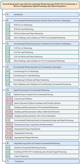
Figure 1.
Structure and organization of the review.
2. Environmental Monitoring Based on Wireless Sensor Network Technologies
The general architecture of an environmental monitoring system based on a terrestrial WSN consists of hundreds or thousands of low-cost sensor nodes located in strategic points of the monitored site (whose position is assumed to be known) and of one or more monitoring centers responsible for collecting and processing all the data acquired by the sensor nodes, as illustrated in Figure 2.
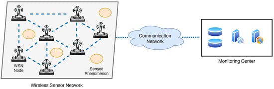
Figure 2.
General architecture of an environmental monitoring system based on a WSN.
Each sensor node in the WSN is a low-power device equipped with:
- A microprocessor unit to control and manage the local tasks and to perform basic computations on the acquired data.
- An internal memory with limited capacity used to store small batches of collected data before transferring them to the monitoring centers.
- A transceiver for establishing communication links with the other nodes in the network and with the monitoring centers.
- A sensing unit equipped with several dedicated sensors (e.g., chemical, thermal, biological) to measure and monitor the environmental parameters of interest.
WSN nodes can collect different types of environmental data in different formats and resolutions, e.g., analog or digital, static or dynamic, spatial or temporal, and images or video sequences, just to name a few. At the monitoring center, the high volume of collected data is properly stored in dedicated databases and processed through high-performance computing systems. Data are typically pre-processed to remove possible outliers before being analyzed and visualized using, e.g., common Geographic Information Systems (GISs), in combination with additional information from satellites (maps) and, possibily, coupled with the predictions produced by spatial–temporal models of the pollutants. The results of the analyses are subsequently made available through specific web platforms to guarantee seamless access to all the authorized entities (private and/or public).
Compared to more traditional systems based on few fixed monitoring stations, WSNs revolutionize the sensing task by enabling an accurate, pervasive, and real-time monitoring of the main environmental processes and parameters thanks to the increased spatial resolution and differentiated sensing capacity of the network. Commercial off-the-shelf (COTS) sensors mounted on the sensing unit of WSN nodes can measure a number of physical parameters such as temperature, humidity, and pressure, as well as some of the most important chemical pollutants. In Table 2, we report the most common type of sensors used in WSN-based environmental monitoring systems, including their operating range and manufacturing technology. For more comprehensive discussions about the various environmental sensors, we refer the interested reader to the dedicated surveys [55,56,57,58,59,60]. In the following, we provide a review of some representative approaches proposed in the domain of WSN-based environmental monitoring, classified based on their fields of application (air, land, or sea). On the basis of the reviewed literature, we then conclude the section by highlighting the common challenges and the main limitations of WSN-based monitoring systems.
Table 2.
Typical sensors used in WSN-based environmental monitoring systems.
2.1. WSN for Air Monitoring
WSN technologies have received significant attention in the area of air environmental monitoring. With the progressive evolution toward the emerging reality of smart cities, monitoring the quality of the air in all its aspects (chemical, electromagnetic, and acoustic noise pollution) in crowded urban areas is becoming a major concern. Indeed, the highly dynamic nature of such environments triggers frequent changes in the concentrations of the air pollutants, which in the worst cases may occur in the scale of few seconds over time and of few meters in space [61]. Enabling real-time air monitoring in these harsh environments through a scalable, reprogrammable and low-cost WSN deployed over traffic/street lights is the objective of some important projects such as [62,63,64]. Another important aspect of WSN-based air monitoring concerns the quite high power and response time required by greenhouse gases sensors (CO, CO, SO, NO, O), especially those based on MOX technology. In [65,66,67,68], such issues are explicitly taken into account at the design stage and solved using a combination of power reduction techniques that operate at both sensors and network levels, also including some context-adaptive strategies [69]. Minimal invasiveness is another desired property when designing and deploying effective WSN-based air monitoring systems, especially for indoor environments. In [70,71,72,73], different multilayer architectures are presented that enable a distributed monitoring of the air environmental parameters using only a limited number of deployed sensors while still preserving the low-cost and flexible characteristics of a WSN. The optimal deployment of WSN nodes for finer spatio-temporal air monitoring is addressed in [74,75,76]. The optimization problem is formulated by explicitly taking into account the dynamic diffusion of the air pollutants, represented by means of atmospheric dispersion models, including also some realistic connectivity issues among the nodes in the WSN. Preliminary experiments on real datasets indicate that the actual sensing capabilities of the WSN are strongly affected by the weather conditions, with the estimation performance that tends to increase when the sensors are deployed at an altitude close to the main concentrations of the air pollutants. Moreover, the deployment costs, which are quantified as the total number of WSN nodes required to guarantee a predefined error-bounded coverage, can be progressively lowered as the number of pollutant sources or the number of emissions from a single source increases.
WSN technologies have also proven their validity in monitoring different sources of environmental acoustic noise (ranging from those generated by common transportation systems to industrial manufacturing and building construction) that can be found in most human-centric areas [38,77,78]. Compared to sensing chemical air pollutants, which involves the processing of separate data from each dedicated sensor, acoustic noise monitoring introduces additional challenges related to the correct separation, classification, and identification of the several noise contributions that are superimposed at the receiving microphones [79]. In this respect, a lot of work has been devoted to the design of advanced acoustic signal processing techniques that elaborate on well-known methods such as beamforming [80], source localization [81], array calibration [82], and noise reduction [83]. An evident trade-off between accuracy and deployment costs tends to emerge from the reviewed literature: on the one hand, approaches such as [84,85,86] consider class-A acoustic sensors to build near real-time maps that provide a detailed analysis of the acoustic environment, including the classification of all the diverse sources of noise. Such approaches are however limited to very small areas (WSNs with less than 10 nodes), being that their costs are prohibitive and do not allow a flexible adaptation of the signal processing algorithms at the sensor9 level. On the other hand, the systems presented in [87,88,89] aim at providing a fairer balance between deployment costs and achieved accuracy by relying on low-cost acoustic sensors that can only measure global aggregated levels of equivalent noise, but they enable a more pervasive installment of the WSN over the monitored area.
2.2. WSN for Land Monitoring
WSN technologies have found several application contexts in the field of soil monitoring. The ever increasing urbanization of the modern society is leading to a significant growth of the total amount of waste produced per year [90], which calls for adequate monitoring systems to supervise the storage, treatment, and recycling processes. Such systems should guarantee that some pivotal parameters (e.g., level of radiation, percentage of chemical and biological pollutants) are within the tolerated ranges and, whenever possible, prevent the illegal dumping of solid/liquid waste in the environment. As an enabling technology of the emerging Industry 4.0 paradigm, WSNs have been employed to monitor nuclear storage facilities [91,92], the disposal of chemical materials and waste [93], and, more generally, harsh industrial environments [94,95]. A common challenge faced in all these scenarios is represented by the extreme environmental conditions in which the WSNs are deployed. More specifically, very high temperatures, hazardous gases and the possible presence of chemical acids in the surrounding of sensors can severely impair the correct sensing capabilities of the WSN. Building a reliable and robust WSN monitoring system in harsh environments has been a topic of interest in the literature [96]. The proposed solutions typically augment the sensing systems by adding multiple backup sensors equipped with supplementary modules. This, however, comes at the price of an increased power consumption, which in turn calls for the necessity of proper energy harvesting technologies [97,98].
WSN monitoring systems play a crucial role also in fostering the prevention, early detection and quick management of natural disasters. Critical though recurrent phenomena such as wildfires can be combated by using WSN monitoring systems based on long-range (LoRa) wireless communication technology, which provides sufficient coverage for small and mid-size areas [99,100,101]. WSN monitoring systems turn out to be effective also for landslides prediction [102]. Due to the several factors that influence these phenomena (e.g., characteristics of soil, altitude, vegetation, etc.), the data collected by the WSN should be fused with geotechnical and hydrological models [103] and further processed within GIS in order to perform accurate analyses [104].
Precision agriculture is another important field of application for WSN-based monitoring systems. Introducing sensing technologies into the basic farming processes, from the optimal provision of soil nutrients up to an efficient management of the irrigation systems and fertilizers, is pushing agriculture toward the new emerging dimension of smart agriculture (also called Agriculture 4.0) [105]. A lot of work has been devoted to the adoption of WSN technologies to monitor the main soil parameters such as the moisture, temperature, pH, and wind direction [39,106], as well as the quality of crops [107] and the efficiency of the irrigation systems [108,109]. From the surveyed literature, it appears that the Arduino platform is one of the most adopted technologies to integrate a variety of soil sensors, while Tiny OS is the leading operating system installed on the WSN nodes. Among the main open challenges, it is worth mentioning the trade-off between the optimal deployment of sensor nodes to guarantee full coverage of the farming area and the choice of the low-power wireless communication technology to overcome attenuations and blockages due to the presence of dense crops.
2.3. WSN for Marine and Water Monitoring
During the last decades, marine environments have been severely threatened by effects related to anthropological activities such as tourism, urbanization, and industry [35,110]. Compared to traditional systems based on oceanographic research vessels, WSNs have provided dramatic improvements in terms of real-time analyses and monitoring of marine and coastal areas: on the one hand, the high cost associated with the startup and maintenance of the vessels is completely avoided [111]. In addition, the higher sensing resolution in both time and space promotes a more timely response against unexpected critical events such as flooding or water contamination [112]. A typical WSN-based marine monitoring system consists of a set of nodes deployed near the coast and/or in strategic points of the sea surface. The general architecture of each WSN node comprises a floating support (usually a buoy) to isolate the main electronic parts and RF communication modules from the water along with a sensing subsystem equipped with underwater sensors measuring different physical parameters such as pH, temperature, pressure, level of salinity, turbidity, oxygen density, and chlorophyll. Differently from land or air applications, WSNs operating in marine environments face three main additional challenges: (i) sensor nodes need to be protected against corrosion and adverse conditions such as tides, high waves, cold/hot currents, and typhoons, which undermine both the stability of nodes and sensing accuracy; (ii) preserving and harvesting energy is of utmost importance since sensor nodes are often deployed in unapproachable points of the sea and use long-range power-hungry wireless communication protocols to send data to the monitoring centers; (iii) underwater communications are highly unreliable due to extremely low channel capacities and high signal attenuations experienced when communicating through water. To address the first issue, biofouling protection capabilities have been added to the underwater sensors [113,114], and more advanced flotating buoys have been designed to better support the sensing nodes [115]. The energetic problems have been tackled by using both overwater [116,117] and underwater solar energy harvesting technologies [118] as well as by leveraging the kinematic energy from waves [119]. For underwater communications, acoustic waves represent the mostly adopted technology, even if they still suffer from high attenuation, significant delays in propagation, and fading effects. In some cases, a combination of optical, acoustic, and electromagnetic communications should be used to overcome the unreliability of the underwater links [120,121], possibly coupled with advanced routing [122] and hop-counting strategies [123] for improved efficiency.
Monitoring the quality of fresh-water courses and related drinkable water supply systems is another appealing application of WSN technologies. Providing clean and controlled drinking water typically involves a manual collection of water samples followed by intensive laboratory-based analyses. These approaches are, however, highly inefficient and expensive and cannot provide real-time information about water quality, preventing the possibility of timely identifying accidental or malicious contamination. In this respect, WSNs provide an important shift in the monitoring paradigm, enabling a real-time, low-cost analysis of the main water parameters (e.g., turbidity, pH, conductivity, etc.) with improved spatial and temporal resolution [36,124]. Given the absence of accurate biological and chemical sensors on common low-cost WSN nodes [125,126], most work in the literature has focused on the design of advanced contamination detection algorithms that properly fuse the different data collected from multiple sensors [127]. This kind of approach intrinsically suffers from increased false alarm rates, which in turn calls for more sophisticated methods that correlate the decisions with additional information coming from other external sources [128].
2.4. Main Challenges and Limitations of WSN Environmental Monitoring
Despite their transversal applicability to almost all the main environmental contexts (from air to land and up to sea), WSN technologies are still subject to a number of important issues that should be carefully considered when employing them for monitoring purposes. The main open challenges and limitations include:
- Power Management and Node Lifetime: The limited autonomy of WSN nodes, equipped with reduced-capacity batteries, is a major concern for WSN-based environmental monitoring systems, especially when nodes are deployed strategically though hardly accessible areas. Sophisticated strategies need to be conceived to ensure minimum energy consumption, with a particular focus on the most demanding RF components. Two main approaches are typically followed: (i) developing energy-efficient algorithms and communication protocols; (ii) using energy-harvesting techniques to restore energy based on solar cells, piezoelectric vibration-based devices, etc. Recently, new approaches for wireless energy replenishment started to be explored, relying on the availability of an additional set of mobile rechargeable units to prolong the lifetime of WSN nodes [129,130]. Preliminary results showed that such methods can significantly extend the duration of the sensing campaigns, thus representing a promising solution for WSN-based environmental monitoring [131].
- Communication Range: Communications in WSNs are typically performed using relatively low-power wireless technologies (e.g., ZigBee), which can only guarantee limited coverage. In most environmental monitoring scenarios, the harsh propagation conditions could lead to frequent obstructions or blockages of communication signals, potentially jeopardizing the whole sensing process. Some attempts have been made to improve the connectivity by studying the optimal placement of sensors under the assumption of some underlying wireless channel model. However, the practical solution adopted in most real deployments is still to increase the density of nodes in the WSN, with a consequent increase in the overall cost. In recent years, the use of connected dominating sets started to emerge as an effective way to reduce routing costs between sensing nodes and to generally improve the communication range, especially when WSN nodes are unevenly distributed over the target area [132,133]. Such approaches can be thus used to support node deployment and to make data collection/dissemination within the network much more efficient [134].
- Sensor Data Quality: Typical low-cost physical and chemical sensors employed for environmental monitoring return measurements that can be highly inaccurate, especially in the presence of miscalibration of the sensing units. Assessing the quality of the collected data becomes a priority when multiple heterogeneous sensors are used to monitor the same environmental phenomenon. Advanced outlier detection and data fusion algorithms are currently under investigation in the literature to avoid instances of a few unreliable measurements compromising the entire acquisition campaign. Accurate time synchronization of all the collected data represents another crucial aspect for obtaining reliable analyses [135]. As a prerequisite for most data-fusion algorithms [136], temporal information is combined with positional information to spatially contextualize the sensed data and outline the spatio-temporal correlations existing among them. This is of particular interest when dense WSNs are employed, for instance, to monitor environmental phenomena over very small areas [137]. In these cases, measurements collected by each WSN node are likely correlated among each other as well as with the measurements carried by neighboring nodes in the network. Notably, accurate clock/data synchronization is of utmost importance when some relevant environmental parameters, inferred from data, are used to detect possible violations of safety-critical thresholds in real-time or used to feed numerical prediction models to assess the possible evolution of phenomena both on a temporal and geographical scale [138,139].
- Reliability and Fault Tolerance: Robustness against possible hardware, software, and communication failures is a crucial aspect for WSNs to be effective in environmental monitoring. Given the low-cost nature of sensor nodes, even common phenomena such as rain, humidity, and wind can induce circuitry faults or frequent system reboots. Guaranteeing a highly reliable WSN is of utmost importance, especially when monitoring dangerous environmental phenomena (e.g., wildfires, water contamination, radiation) in real time, which requires that any potential emergency be promptly reported to the competent authorities. Enhanced reliability and fault tolerance are typically achieved by introducing redundancy of the main hardware components and by designing proper routing mechanisms and topology control schemes.
- Scalability and Cost: Most of the main environmental phenomena usually occur on a large spatial and temporal scale, following highly dynamic evolution processes. Monitoring them would thus require scaling up the WSN so as to cover vast areas with a significant number of sensors. Unfortunately, it is not often possible to deploy a dense WSN over a large-scale environment, for both physical and economic reasons. This is widely confirmed by the reviewed literature, where it emerges that WSNs are mainly used for monitoring relatively small areas.
3. Environmental Monitoring Based on Unmanned Aerial Vehicle Technologies
Over the last decade, UAV systems have progressively evolved toward a level of maturity that makes them powerful and versatile platforms for improving environmental monitoring tasks [40,41]. Figure 3 illustrates a general UAV-based monitoring architecture, which comprises a swarm of UAVs acquiring data over a specific monitored site defined by a set of target points, coordinated by one or more ground control stations, which are also responsible for the processing and preliminary analysis of the collected data. UAVs are available in the market under different models based on the type of propulsion (fixed wing or multi-rotor) and the maximum payload that can be carried. In Table 3, we report the main type of UAV platforms used for environmental monitoring purposes, together with their average coverage and main characteristics.
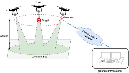
Figure 3.
General architecture of an environmental monitoring system based on UAVs.
Table 3.
Common UAV platforms for environmental monitoring.
UAV nodes are equipped with a local microprocessor, an internal memory, a sensing and communication unit, as well as by some additional subsystems:
- A navigation and guidance unit responsible for obtaining real-time geolocation information using a GNSS receiver, usually coupled with a set of inertial and odometry sensors (e.g., accelerometer, gyroscope, etc.), as well as ensuring that a predefined trajectory is followed according to a specific path-planning strategy (mission).
- A propulsion unit using engines, motors, and batteries as power sources, as well as propellers or propulsive nozzles to generate and control the UAV motion.
UAV systems exhibit excellent monitoring and sensing capabilities: indeed, thanks to their aerial inspection ability and flexible characteristics (small size, rapid maneuvering), wider areas of interest can be covered in a timely manner, guaranteeing at the same time accessibility also to sites that would be inaccessible for other technologies such as WSNs or fixed monitoring stations. Although optical and multispectral/hyperspectral cameras remain the primary source of data on UAV nodes, other sensors such as thermal cameras, LIDARs, and gases sensors can be mounted as well. We summarize in Table 4 the most common types of sensors used in UAV-based environmental monitoring systems and refer the interested reader to [140] for a comprehensive review. It is worth noting that some of the sensors can be equipped only on specific types of UAVs, mainly due to the still too-high weight, cost, and maintenance of some components.
Table 4.
Typical sensors used in UAV-based environmental monitoring systems.
Compared to the more traditional manned airborne systems or satellite systems, UAV systems represent a cost-effective technology able to provide acquisition campaigns at an increased spatial and temporal resolution, offering the possibility to accurately track the dynamics of the main environmental processes occurring at very fine scales. High flexibility and easy adaptability to different application contexts make them suitable candidates to meet some of the crucial requirements of environmental monitoring: first, they enable real-time inspection of targeted areas thanks to their ability to perform rapid and repeated acquisitions of environmental data. Second, monitoring of hazardous or contaminated sites becomes possible using UAVs, with practically no risks for human operators. Third, the possibility to quickly reschedule UAV missions in the presence of unfavorable meteorological conditions (e.g., cloudy, rainy, etc.) allows for overcoming the main limitations of both airborne and satellite systems. In addition, UAV operations can be in principle guaranteed over the whole day and not limited only to specific hours as is the case of most satellite systems, enabling in turn a continuous environmental monitoring. Particularly, the costs involved in the deployment of a UAV-based monitoring system are not a limiting factor as for airborne or satellite systems: indeed, the main expenses are only linked to the initial investment in terms of hardware, software, and on-site equipment.
The above-discussed advantages, combined with the continuous evolution in the miniaturization of electronic and sensor technologies, led UAV systems to be widely applied across different domains of the environmental monitoring. In the following, we provide a review of some representative approaches proposed in the literature, classified based on their fields of application: (i) air monitoring, (ii) land monitoring, and (iii) water/marine monitoring. On the basis of the reviewed literature, we then conclude the section by highlighting the common challenges and the main limitations of UAV-based monitoring systems.
3.1. UAV for Air Monitoring
Although UAV technologies are mainly recognized for bringing disruptive enhancements to land and maritime monitoring, their aerial inspection capabilities have opened a new frontier also in the field of air pollution monitoring. Some experimental campaigns, conducted in crowded urban areas, revealed that the level of expansion of the main atmospheric aerosols and gases varies dramatically with the relative elevation from the emitting source. Therefore, monitoring the air pollution only at a ground level (in the order of 1–5 m) could not be sufficient to carry out an accurate air quality assessment. In these contexts, one or more UAV nodes equipped with dedicated gases sensors (as those described in Table 2) can be employed to monitor and track the pollutant concentrations at different altitudes [141,142], delivering at the same time richer real-time information that can be stored and used for long-term analyses [46,143]. Given the quite limited payload that needs to be shared among multiple sensors, some research efforts have been devoted to the design of lightweight gases sensing units for UAV nodes [144,145]. Finding the optimal placement of air monitoring sensors on UAV platforms is another challenging issue, given that the sampling and estimation processes are strongly affected by the dynamic nature of the wind and by the vortex fields generated by the propellers [146,147]. The high spatial and temporal sensing capabilities of UAV nodes have been also employed to build fine-grained air quality index (AQI) maps. Accurate profiling of the air pollution in urban/suburban environments can be achieved in nearly real time [148,149,150], especially when the AQI maps are combined with statistical plume models (such as the Gaussian) that characterize the physical dispersion in the air [151].
UAV nodes equipped with miniaturized infrared thermal cameras offer the possibility to enhance tasks related to the microthermal environmental monitoring, which consists in providing high-resolution analyses of the land surface temperatures and their variations, even at a microscopic level [152]. This information, combined with data related to humidity, solar radiation, and wind speed, is used to support important services such as weather forecasting or to infer the chemical composition of clouds (e.g., near a volcano, or after a chemical disaster) [153].
In recent years, some studies started to investigate the potential of exploiting the flexibility of UAV sensors to perform spatial, temporal, or spatio-temporal spectrum sensing, with the aim of revealing and possibly localizing sources responsible for electromagnetic pollution [154]. The same principle has been applied for monitoring acoustic noise in urban and suburban areas, leveraging UAV nodes equipped with an array of microphones. However, the proposed solutions are still at a preliminary stage, with such contexts being much more challenging to handle due to the presence of additional disturbances such as the wideband noise induced by the propellers and the narrowband noise generated by the engines [155].
3.2. UAV for Land Monitoring
UAV technologies have radically revolutionized the panorama of land environmental monitoring, enabling new horizons that were unconceivable until only a decade ago. The undisputed widespread use of such technologies across a wide range of soil monitoring tasks is strictly correlated with the progresses in the miniaturization and portability of RGB cameras and multispectral/hyperspectral imaging technologies, which allow to bridge the gaps with conventional satellite or airborne remote sensing platforms while providing a cost-effective way to obtain data at high spatial and temporal resolution [156,157]. By inspecting target areas at a very fine scale, UAV platforms are foreseen as potential tools to detect and counteract the illegal dumping of solid/liquid waste in the environment [158,159], for actively monitoring the operations in existing landfills [160], and for general prevention of soil contamination [161]. Preventing the diffusion of unauthorized constructions or their illegal demolition is another important application field for UAV-based monitoring systems [162]. From the surveyed literature, it emerges that these monitoring problems can be addressed using statistical change detection approaches operating on a temporal series of images or video sequences. Specifically, the availability of accurate a priori geometrical information (e.g., digital surface maps), possibly in combination with real-time kinematic information from the onboard inertial sensors, is a necessary ingredient for effective detection of soil contaminants with reduced false-alarm rates. Furthermore, since high resolution UAV images could likely trigger many undesired changes, advanced registration algorithms that properly align images acquired at different elevations and under different perspectives should be used at the pre-processing stage. In particular, when processing spectral data, change detection algorithms should expect higher in-class variances due to different acquisition conditions (e.g., illumination, shadows) and more complex scenes at hand [163].
UAV systems represent an indispensable technology to support onsite real-time monitoring of wildland areas subject to risks of natural hazards or disasters. Thanks to their aerial capabilities, environmental operations can be quickly conducted even in situations in which ground-level technologies could not be applicable and human intervention is too dangerous. The most prominent use case of UAV-aided natural disaster monitoring is the recurrent problem of forest wildfires [44]. Typically, high-resolution images acquired by RGB or infrared cameras are combined with information from the onboard inertial sensors and processed through advanced image processing algorithms to detect wildfires at their early stages and track their temporal evolution. Traditional computer vision approaches such as median/Gaussian filtering, image segmentation, and color analysis (in both RGB or HSV spaces) have been successfully applied to perform smoke detection and successive identification of the fire location in terms of altitude, latitude, and longitude [164,165]. When the ground control stations are equipped with significant computational power, deep learning algorithms such as convolutional neural networks and deep neural networks with an underling YOLOv3 architecture can be used to achieve improved flame and smoke detection performance at reduced false-alarm rates, even in the presence of adverse cloud and sunlight conditions, as well as undesired reflections from objects in the scene [166,167,168]. Image/video-based analytics have proven their effectiveness mainly for wildfires localized in relatively small areas. When the wildfire spreads over much larger scales, different measurements (e.g., temperature, wind) collected by a swarm of UAVs are fused within advanced filtering approaches (e.g., Kalman-based) that include wildfire propagation models such as the Rothermel or the Canadian forest fire behavior [169,170]. In addition to data processing, suitable distributed control frameworks need to be devised to design time-varying trajectories that enable a close monitoring of wildfires through multiple coordinated UAVs while minimizing the risk of in-flight collisions or damages, as well as to reduce the total number of transmissions toward the ground control stations [171,172]. Based on these advanced control schemes, some proactive approaches have started to appear in the literature that exploit the payload of UAVs to drop fire retardants or extinguishing agents at the epicenter of the wildfire [173].
Besides wildfire monitoring, UAVs have been employed to counteract geological hazards such as landslides using both optical [174] and thermal remote sensing techniques [45], and even to perform vulnerability analyses after natural disasters such as tornados [175]. Apart from the benefits brought to each individual application context, a common advantage of using UAVs in natural disasters monitoring, from prevention to recovery, is their ability to rapidly reproduce high-resolution maps of the target areas, a task usually called land-use land-cover mapping (LULC). Such maps, which can be either two-dimensional (surfaces) or three-dimensional (volumes), are at the basis of any emergency response application supported by a UAV system [20].
Proliferation of UAV systems brought new opportunities also in the field of vegetation analysis for both natural and agricultural environmental aspects [176]. Assessing vegetation health is a complex process that requires a combination of several indexes extracted from multiple sensors (ranging from optical images, infrared, and multispectral/hyperspectral). UAV platforms have been used to retrieve important information from natural habitats and ecosystems, including the monitoring of plant infection [177], average tree mortality [178], and level of diffusion of serious diseases such as the Xylella fastidiosa [179], with a granularity that can even reach the tree-level. Across all the considered technologies, hyperspectral imaging turned out to be a preferable tool to rapidly detect the level of vegetation stress based on the examination of pigments and chlorophyll [42]. On the other hand, a combination of data from optical cameras and LIDAR represents the most reliable solution when a 3D reconstruction of trees and crops is the main objective of the monitoring task.
Precision agriculture is another application context that can reap great benefits from the use of UAV-based monitoring. Compared to more traditional systems (e.g., satellite-based), UAVs provide field-level analyses that can be fruitfully exploited for the early diagnosis of agricultural problems, enabling in turn timely corrective actions from the farmers and, consequently, a significant reduction in both costs and environmental impact [180]. Prominent examples concern the use of UAV platforms to monitor the status of crops [176] and the quality of the soil [181], which allows for obtaining accurate predictions of the ultimate yield. From a technological point of view, RGB and thermal data have proven their usefulness for quantifying the main soil moisture contents, while accurate estimation of the water contents in the subsurfaces can be achieved by additionally exploiting mathematical models (e.g., the Soil Moisture Analytical Relationship) that link measurements collected at the surface to the parameters of interest [182].
3.3. UAV for Marine and Water Monitoring
Coastal and marine environments represent exciting application fields for the use of UAV monitoring technologies. Despite that most of the aerial remote sensing techniques in these contexts are based on satellite or airborne systems, mainly due to their wide coverage, UAVs open up a new set of significant opportunities to overcome the still too-limited imagery resolution, as well as the coarse and often discontinuous acquisition rate. By exploiting the improved spatial and temporal resolution and the availability of multiple sensors, UAVs can be used to carry out in-depth water quality analyses based on multiple correlated parameters [183]. More specifically, peculiar characteristics of the water surface reflectance captured by hyperspectral cameras can be used to detect suspended solids [184], particulate matter [185], and even toxic agents (chemical, biological) [186], while machine learning tools (e.g., SVM) turned out to be very powerful solutions to identify the presence of oil spills in optical images [187,188]. Using the Nemerow index and traditional regression techniques, the presence of smelly water can be readily identified [189], and the level of water transparency can be assessed in near real-time [190]. Spectral cameras carried by low-cost UAVs have been also used to monitor the sedimentation levels in natural reservoirs, and to assess the presence of submerged vegetation and algae species that are considered microbiological indicators of good water quality [191]. Notably, UAV technologies recently started to be adopted as a means to counteract the main phenomena of seaside degradation such as the dispersion of litters on the beach [192], or the uncontrolled dumping of plastic debris that are seriously threatening the aquatic wildlife [193].
The integration of water observations collected from UAV sensors with hydrological models allows for significantly enhancing the accuracy in describing the dynamics of rivers, lakes, and seas, enabling in turn a more effective monitoring of critical phenomena such as inundations and floodings. A number of proofs of concept have been proposed in the literature to demonstrate the feasibility of applying UAV optical techniques to perform distributed estimation of kinematic parameters such as the velocity of surface flow fields (e.g., using Large-Scale Particle Image Velocimetry) [194], which are used to delineate candidate flooding zones. Interestingly, some experiments revealed that an accurate survey can be obtained by just letting the UAVs hover for a few seconds around the target area, provided that orthorectification and photometric calibration phases have been correctly performed. When advanced deep learning algorithms are used to process and classify RGB images, accurate mapping and tracking of the flood routing and its probable extent can be inferred in near real-time [195]. Proper fusion of data coming from different sensors and an accurate modeling of the main hydrological parameters and their mutual dependencies remain the main open challenges to be faced before UAV platforms can be fully considered to support civil protection agencies in critical water monitoring tasks.
3.4. Main Challenges and Limitations of UAV Environmental Monitoring
The huge potential of UAV technologies is largely demonstrated by the several environmental application fields in which they brought not only significant improvements, but also radical revolutions. At the same time, we are witnessing the emergence of a significant number of methodologies based on specific combinations of hardware technologies (e.g., sensors, platforms) and algorithms (either for path planning, sensor calibration, or data processing) that are tailored only to the peculiar needs of each selected case study. In this respect, a major substantial challenge that should be addressed concerns the proper harmonization and standardization of processes involving the application of UAVs for environmental monitoring purposes. In addition to such a general challenge, from the analysis of the reviewed literature, some common though important open issues tend to emerge:
- Policy and Regulations for UAV Operations: The operations of UAV platforms are subject to regulations and restrictions imposed by governments that generally differ across different countries. Such limitations are imposed to guarantee the general public safety (especially in the presence of damages of the UAV platforms) and to ensure that the UAVs do not interfere with other aerial systems that share the same flight areas. To date, most of the regulatory frameworks do not allow fully autonomous UAV missions but require the presence of a licensed pilot to carry out even the most basic operations. Since these requirements inherently restrict the minimum distance at which UAV platforms can sense environmental data (known as Ground Sample Distance (GSD)), they represent one of the greatest obstacles toward a diffuse use of UAVs for environmental purposes.
- Sensor Calibration and Error Correction: Most of the lightweight sensors designed for UAV platforms typically experience significant geometric and spectro/radiometric limitations, calling for the need of adequate self-calibration and pre-processing procedures. Radiometric calibration includes several steps (such as the adjustment of colors, removal of noise, and deblurring) and requires the presence of spectral targets with known reflectance properties. Unfortunately, such a process is severely threatened when UAVs operate in adverse weather conditions (rain, wind) due to induced undesired spectral effects such as variable illumination, alterated reflectivity of materials, partial absorption, etc. On the other hand, the rapid maneuvers and frequent changes in flying altitude and orientation typical of the motion of UAVs introduce undesired impairments such as lens distortion and misalignment of the fundamental camera parameters (e.g., focal length, distortion coefficients, etc.) that should be compensated by means of a geometric calibration process. The overall correction process is known as orthorectification and represents one of the main research topics [196].
- Flight Time and Path Planning: The limited flight time of UAV platforms represents another crucial aspect that should be carefully taken into account when planning an environmental sensing campaign. This problem can be generally managed in two alternative ways: one possibility is to devise optimized path-planning strategies that take as input the extent of the area under investigation and the energy constraints of each involved UAV node and produce a set of trajectories (expressed as sequences of points of interest, as shown in Figure 3) that try to guarantee a satisfactory trade-off between coverage, sensing accuracy, and total duration of the data acquisition campaign. In this respect, recent studies have demonstrated that even the specific geometry of the flight path, passing through all the selected points of interest, can also have a strong impact on the achievable coverage and timely data acquisition capabilities of UAVs [197]. In particular, simple geometric flight patterns easily meet short path length and minimum mission execution time requirements but may conflict with other requirements such as energy consumption, being that short and simple paths are more likely to contain abrupt maneuvers, which in turn consume more energy [198]. A second possibility consists in leveraging the recent advances in lightweight battery technologies, which promise extended flight durations from about 1 h up to 5 h if solar-panel-based energy supplying systems are also integrated onboard. Overall, the experimental campaigns conducted so far have revealed that current UAV technologies can be considered cost-effective monitoring tools mainly for areas of quite limited extent (0.2 km), while for larger areas, other technologies need to be adopted as complementary solutions.
- Localization and Tracking: Accurate estimation and tracking of the position and orientation information of UAVs over time is a fundamental prerequisite for all tasks involved in the monitoring process, from the initial pre-flight path planning until the data processing and subsequent analyses stages. On the one hand, ground control stations need to accurately predict UAV trajectories in order to design distributed control strategies that effectively coordinate the monitoring operations, especially in the presence of swarms of UAVs, without the risk of collisions or damages. On the other hand, any aerial photogrammetry-based method strongly depends on the accuracy of the georeferencing process. This task, also called registration, consists in associating the collected digital images to physical locations in the space through the definition of a set of ground control points (GCPs). Current practices in UAV enviromental monitoring consider the use of onboard GNSS and inertial measurements combined with the navigation and guidance unit to directly determine the UAV’s position and orientation [199]. However, such solutions turn out to be inaccurate or even unavailable in some practical operational scenarios since most of the hardly accessible sites monitored by UAVs are usually also GNSS-denied environments.
4. Environmental Monitoring Based on Crowdsensing Technologies
The pervasive, almost ubiquitous spread of smart mobile devices (smartphones, smartwatches, wearables, in-vehicle, etc.) featuring enhanced wireless communication capabilities and a rich set of built-in sensors (e.g., cameras, GPS, accelerometers, microphones) is progressively pushing the well-known benefits of the crowdsensing paradigm, in terms of large-scale sensing and information sharing, also into the context of environmental monitoring [47,50]. The general architecture of an environmental monitoring system relying on crowdsensing technologies consists of a pool of mobile smart devices leveraging their embedded sensors to collect different environmental data across different areas of the territory, according to the activities of the specific users (e.g., people moving in an urban center, vehicles traveling in forest or coastal areas, etc.), which are then sent to dedicated monitoring centers that are responsible for storing, integrating, and analyzing the huge volume of crowdsensed data, as shown in Figure 4. Sensed data are generally transmitted using different communication technologies, from ad hoc wireless networks (e.g., Bluetooth, Wi-Fi) to infrastructure-based networks (e.g., cellular 3G/4G/LTE). Thanks to the rapid evolution of portable sensor technologies, smart devices are equipped with an impressive number of built-in sensors that can be used to sense and monitor different physical parameters, e.g., electromagnetic fields, sound, temperature, humidity, etc. In Table 5, we summarize the most common types of sensors currently found in crowdsensing-based environmental monitoring systems.
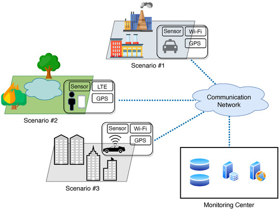
Figure 4.
General architecture of an environmental monitoring system based on crowdsensing.
Table 5.
Common sensors used in crowdsensing-based environmental monitoring systems.
Crowdsensing technologies offer enhanced monitoring capabilities compared to more traditional systems such as fixed stations and satellites. The key idea consists in building a collective view of the environment by exploiting data sensed by citizens in their daily routines. This can be practically implemented by using the concept of crowdsourcing: a formidable task such as the large-scale monitoring of the environment, traditionally performed by specialized and complex infrastructures, is distributed among ordinary users that leverage their own smart devices to sense data. In this respect, two different sensing modalities can be adopted: (i) participatory sensing in which users voluntarily collaborate to accomplish the sensing tasks, possibly receiving some kind of reward for their contribution; (ii) opportunistic sensing where conversely users do not need to undertake specific actions and are even unconscious of the sensing process that is passively carried out. The crowdsensing paradigm brings two main advantages to the environmental monitoring field. First, the frequent temporal and spatial variations of natural phenomena can be more accurately captured by fusing the big environmental data collected across separated spatial locations at different time instants. This huge amount of information can be used to extend the scale of the sensing campaign, overcoming the often limited spatial and/or temporal coverage provided by other existing monitoring systems without any additional deployment cost. Second, introducing human intelligence into the sensing process complements the information collected by the sensors with a much deeper understanding of the operational contexts [200].
Although the general architecture in Figure 4 may somewhat resemble that of a WSN-based monitoring system, profound differences can be found between the two technologies. First, WSN nodes are deployed over fixed locations and are tailored to specific types of environmental analyses. Their specificity usually leads to data of higher quality, but at the same time involves increased cost for the deployment and management of nodes. Conversely, since crowdsensing nodes are general-purpose mobile devices equipped with different kinds of sensors, they can be reused for different environmental monitoring tasks without requiring the deployment of specific infrastructures, thus representing an appealing cost-effective solution. Second, WSNs nodes are low-cost devices with very limited processing, memory, and energy, which constrains their local capabilities and makes it difficult to perform continuous monitoring tasks. On the other hand, crowdsensing nodes benefit from improved processing capabilities and the possibility of recharging their own batteries, which significantly extends their operational range. Another important difference concerns the limited monitoring scale of WSNs compared to crowdsensing. A study conducted in [201] revealed that about 100,000 WSN nodes would be required to enable environmental monitoring of a mid-size city, while guaranteeing full spatial coverage and sufficient connectivity with the monitoring stations. In particular, the inherent mobility of crowdsensing nodes (along planned or random trajectories) can be exploited to sample natural phenomena at an increased spatiotemporal resolution [202].
In the following, we provide a review of some representative approaches proposed in the literature, classified based on their fields of application (air, land, or sea). On the basis of the reviewed literature, we then conclude the section by highlighting the common challenges and the main limitations of crowdsensing-based monitoring systems.
4.1. Crowdsensing for Air Monitoring
Crowded urban areas are recognized among the main sources of worldwide air pollution, but at the same time are the perfect places where several crowdsensing nodes can be recruited [203]. People equipped with smart devices, vehicles routinely traveling along city streets, taxis, buses, and any transportation system at large are only some prominent examples of the multitude of crowdsensing nodes that can be exploited to estimate sources of air pollution and to infer their potential impacts on human exposure, allowing in turn to mitigate and prevent their negative side effects [204,205]. Thanks to the availability of a huge amount of urban environmental data, a number of pilot research projects have been funded in recent years with the aim of assessing the feasibility of air monitoring via participatory crowdsensing. The HazeWatch application, developed as one of the first crowdsensing-based approaches, is nowadays actively used by the National Environment Agency of Singapore [206]. GasMobile, CommonSense, Third-Eye, AirSense, and 3M’Air are other examples of monitoring systems that demonstrate the possibility of building accurate air pollution maps using only off-the-shelf sensors available on citizens’ smart devices [207,208,209,210,211]. Focusing on vehicles and road transportation systems as crowdsensing platforms, the paradigm of drive-by sensing has been coined, and interesting experimental campaigns have been conducted in New York City to first quantify the sensing power of crowdsourced vehicle fleets [212,213] and then assess how the different mobility patterns (either predictable or completely random) impact the discrete-time sampling process [214,215]. Some theoretical work considered the adoption of a network of crowdsensing vehicles and mapped the problem of estimating the air pollution levels into a problem of spatial field reconstruction from samples randomly gathered in a multidimensional space [216]. Improved accuracy and efficiency can be obtained when the correlations among the sensed data are explicitly considered in the model and the unsensed regions are properly characterized [217]. By exploiting analytical models for the variations of the air pollutants concentrations, a cost-effective balance between performance in terms of joint sensing accuracy and communication costs using a vehicular sensor network can also be achieved [218]. In the presence of a sparse number of crowdsensing nodes, compressed sensing techniques can be employed as viable tools to reconstruct accurate air pollution maps using only a small selected set of samples [219,220].
In addition to air pollution monitoring, an increasing number of environmental applications harness microphones embedded in mobile crowdsensing nodes to measure the levels of ambient acoustic noise (e.g., generated by an intense urban traffic) and to infer fine-grained noise maps by fusing the aggregated information at both geographical and temporal levels [221]. Citizens’ mobile phones are the primary sources of noise measurements used across a number of important projects such as NoiseTube [222], NoiseMap [223], NoiseSpy [224], and 2Loud [225], just to mention a few. In most of the considered experimental campaigns, it has been shown that recording the sound pressure signals at frames of about 1 s (with 48 kHz sampling rate and quantization between 16 and 32 bits) is sufficient to enable an accurate prediction of people’s exposure [226] and to localize the main sources of acoustic noise [227]. Compressive sensing techniques turned out to be effective also in recovering noise maps when the number of crowdsensed nodes was very limited and the available samples were incomplete [228]. Noise features can be estimated at a significantly improved granularity (e.g., road level) when the measurements collected by crowdsensing nodes are coupled with advanced noise simulation models [229]. Once the accurate and large-scale noise maps have been reconstructed, advanced analytics can be applied to support proactive interventions aimed at abating noise annoyances [230].
A less investigated but still very promising application field concerns the use of crowdsensing nodes to actively monitor the levels of electromagnetic pollution [231,232]. Received signal strength (RSS) measurements opportunistically gathered from surrounding Wi-Fi access points have been used to build accurate maps of the electromagnetic environment, providing real-time information on the instantaneous power levels of each transmitting source [233,234]. A recurrent issue in this field is how to ensure the trustworthiness of the identified electromagnetic pollution sources while explicitly taking into account the intrinsic inefficiency of the sensors (e.g., antennas) used by crowdsensing nodes [235]. Some work tried to tackle this issue by formulating the spectrum sensing problem as a robust optimization problem, using a generalized modeling approach to take into account the possible presence of incomplete [236], abnormal, or untrustworthy data [237], also including possibly malicious users [238]. Another interesting solution considered the application of a maximum likelihood ratio test over a binary hypothesis, where the non-null hypothesis denoted the effective presence of a non-negligible source of electromagnetic pollution. To explicitly include possible sensor inefficiencies, an expectation-maximization (EM)-inspired approach has been applied to alternate estimation of the probability of successful source identification with the estimation of the sensor efficiency. To further increase the source identification accuracy, the maximum likelihood ratio test can be repeated multiple times as a sequential probability ratio test (SPRT) [239]. Recently, some preliminary work investigated the adoption of deep learning approaches to cope with the presence of very few crowdsensing nodes, especially when operating in harsh propagation environments [240].
4.2. Crowdsensing for Land Monitoring
The widespread availability of crowdsensing platforms gathering environmental data across different physical locations (from urban to rural areas) can offer an important support for monitoring the state and quality of soil parameters and to combat land degradation at large. A successful example in this field is the Danger Maps project developed in China, which is a crowdsensing-based monitoring system whose primary goal is to stimulate citizens in reporting the presence of sources of soil pollution such as illegal garbage dumps generated by toxic-waste treatment facilities, oil refineries, and power plants [241]. A single alert can be quickly triggered by simply reporting a textual description of the pollutant sources, possibly together with pictures captured via the embedded camera. Following the same line of Danger Maps, a general paradigm called citizens as sensors was recently introduced, which aims at actively involving citizens in the fight against land degradation [242], from monitoring the quality of the road surfaces [243] up to facing the rising threat of trash dumping [244].
The ever-increasing number of smart devices disseminated worldwide, combined with the almost ubiquitous availability of mobile communication networks, is opening new opportunities for the use of crowdsensing monitoring techniques to foster the prevention, early detection, localization, and management of large-scale natural disasters. The main advantages reside in the possibility to exploit real-time and geolocated information provided by users to delimit areas that deserve careful attention from the emergency response teams. For instance, some authorities started to consider the potential of such a paradigm to counteract wildfires [245]. While the idea of engaging citizens with their smart devices in the data-gathering process is relatively straightforward, several practical aspects need to be taken into account to guarantee timely and accurate detection of wildfires events, so as to minimize the probability of large-scale damages. More specifically, the crowdsensed data need to be properly processed to extract meaningful information: first, a preliminary coordination strategy needs to be conceived in order to identify the most appropriate type of data to be collected and, consequently, the characteristics of the candidate crowdsensing nodes. Then, the acquisition campaign should be carried out by including appropriate mechanisms to manage underlying non-idealities such as sensor failures and user errors, both accidental and intentional [246]. At the end, some kind of pre-evaluation of the collected data is required to select the most informative sources: Naive Bayes classification has been used to rank the reported data based on the user credibility [247], while multiple binary hypotheses tests have been employed to estimate the probability that the same wildfire event occurred on multiple locations of interest [248]. Social networks represent another valuable source of crowdsensed data but require additional data mining techniques to convert users’ public posts (e.g., Facebook, Twitter, Instagram, …) into meaningful features that can be used in the processing steps [51,249,250]. From an algorithmic perspective, the support vector machine (SVM) classifier has been largely used to map posts over social networks into textual features [251], possibly in combination with a natural language processing method such as the Bag-of-Words to extract additional information conveyed through shared videos [252]. Furthermore, some modeling approaches such as logistic regression may be required to track how the information flows across different groups of users and assess its correctness [253]. To generate knowledge from the aggregated data while satisfying the real-time requirements of wildfire management, efficient data-fusion techniques that operate over short time windows (comparable with the dynamics of the wildfire) must be applied to combine the different categories of reported data and simultaneously filter out any redundant information. The final analyses and visualization phases are responsible for superimposing the positions of identified wildfires on real-time maps and to infer the envelope of the interested areas, predicting the possible evolution of the fire based on propagation models fed with local meteorological data [254].
Besides wildfire monitoring, participatory crowdsensing has been employed for near real-time detection of other disaster events such as earthquakes [255], landslides [256], and floods [257]. A common approach in these contributions is to consider only sensor readings with an associate position information (either from GPS or cellular networks). Since such phenomena cannot be easily characterized with a single analytical model, stochastic inference tools such as the particle filter are used to reconstruct a spatial model from the collected observations, which is then used to estimate an approximate location of the hazard event.
Very recent studies have foreseen crowdsensing monitoring techniques as indispensable components in the emerging contexts of smart agriculture [49]. Thanks to the evolution in the worldwide economy, even in underdeveloped countries, an increasing proportion of farmers have at least one smart device and would be willing to use it for further increasing their income [258]. Compared to other application fields, in which citizens may not have a specific expertise, the experience accumulated by farmers during their professional career represents an extremely valuable source of information that can be deeply integrated and used as a boosting component in most farming processes. Although this paradigm, also known as farmers as sensors, is still in its infancy, very promising directions have already been investigated, such as the identification of possible crop pests and diseases via deep learning approaches applied to recorded photos and videos [259,260], prediction of possible agricultural disasters due to adverse meteorological conditions [261], accurate estimation of the cultivated lands by exploiting farmers’ mobility [262], assessment of the quality of fruits [263], as well as for planning the annual production in all its phases [264].
4.3. Crowdsensing for Marine and Water Monitoring
Crowdsensing technologies represent a valuable resource to enhance the study and monitoring of seas, lakes, and oceans, with the aim of forecasting possible catastrophic events, to support marine-related activities, and to prevent the environmental degradation of any marine or coastal area at large. Interesting research projects have been funded in recent years, especially in the south of Italy: the University of Cagliari, in collaboration with the Mediterranean Sea authorities, designed and validated a crowdsensing-based monitoring system whose main goal is the safeguarding of coasts against the negative effects caused by the raising phenomenon of mass tourism [265]. By integrating feedback sent by users in the monitoring processes, the system is able to accurately predict the actual occupancy rate of bathing establishments and to identify potential sources of littering. The SmartWave project developed by the University of Palermo (Sicily) is another example of a crowdsensing-based prototype that aims at monitoring the main phenomena characterizing the marine environment. To do so, the major research challenge was to design a data fusion module able to standardize and properly combine the huge amount of heterogeneous, possibly incomplete data collected by citizens [266]. A pilot study has been conducted in Greece to investigate the impact of the COVID-19 pandemic restrictions on tourism demand, and a prototype platform that exploits data crowdsensed by volunteer tourists has been developed to monitor a 16,000 km extended coastal zone [267].
Participatory crowdsensing can play an important role also in predicting and minimizing the impacts of some catastrophic marine events. By integrating crowdsensing monitoring with the use of social media, a more accurate estimation of fundamental geophysical models for the propagation of oil spills in the oceans’ surfaces can be obtained. A prominent example has been reported in [268], where images related to the disaster of the Deepwater Horizon in the Gulf of Mexico were collected from Flicker and used to support the forecast of the GNOME model parameters. Interestingly, the use of metadata information (location and time) associated with the crowdsensed images brought significant improvements in the estimation of the rate of oil spill diffusion and the coefficient of diffusion while also highlighting important correlations between currents and surface winds. Another relevant application field is the context of flood risk management. Due to the severe climate changes experienced in the last few years, flood occurrences increased considerably, and containing their effects requires up-to-date and accurate knowledge of some critical environmental state variables [269]. Some studies have demonstrated that smartphones can estimate important parameters such as water levels, with an accuracy that can even achieve the cm level when the images captured by cameras are fused with the builtin orientation sensors [269,270]. The main drawback resides in the still too-involved operations that are demanded of the volunteers in order to carry out meaningful measurements. Moreover, few maps representing an updated overview of the flood risk areas are available.
Monitoring the fresh water sources and related infrastructures is another potential application field of crowdsensing technologies. Preliminary work investigated the behavior of the involved citizens when solicited to participate in the sensing campaign [271]. A data analysis conducted using the theory of planned behavior demonstrated that some demotivational factors could severely impact the willingness of citizens in reporting their collected information. To overcome such a drawback, a gaming approach for urban water crowdsensing has been designed and validated in [272], where citizens are provided with a kind of entertainment by means of a gamified interaction with the environment. Although promising, such an application context is, however, less investigated in the available literature.
4.4. Main Challenges and Limitations of Crowdsensing Environmental Monitoring
Undoubtedly, crowdsensing technologies represent a very versatile solution to improve most of the processes involved in the environmental monitoring tasks, as they transversally impact all air, land and marine scenarios. Compared to the other existing technologies, they provide two fundamental benefits: (i) cost-effectiveness, as the sensing processes are entirely run on users’ mobile devices, which leverage their embedded sensors to sense or generate data, and hence they do not require the deployment of additional infrastructures, eliminating the need for purchasing new monitoring devices; (ii) scalability, since the number of crowdsensing nodes recruited for the monitoring tasks can grow significantly according to the willingness of citizens to contribute to the measurement campaigns, enabling in turn a potential large-scale analysis of the main environmental phenomena thanks to the improved spatial coverage. However, from the analysis of the surveyed literature, it can be observed that some important research challenges still need to be properly addressed:
- Incentive Mechanisms: To be effective, crowdsensing-based environmental monitoring must rely on a sufficient number of users participating in the sensing campaign. Although the timely topic of environmental protection may stimulate the general interest, people can be reluctant in providing some kind of “access” to their own smart devices, for either ethical or private concerns. In addition, for some specific monitoring tasks, the sensing process could require an intensive use of processing and communication resources, resulting in an inevitable consumption of energy for users’ devices [273]. Indeed, users may be asked to move to specific target locations and to perform certain actions in order to accomplish the sensing task, possibly deviating from their planned routine. Therefore, suitable incentive mechanisms need to be devised for compensating users’ contributions and promoting their participation in the monitoring tasks. Research approaches can be categorized in two main groups: monetary incentive mechanisms, in which users are paid with a monetary reward [274,275], and non-monetary mechanisms where instead users are rewarded with alternative incentives such as gaming, social entertainment, or virtual credits (e.g., coupons) [276,277]. In the former case, the monitoring system has the additional burden of implementing suitable automatic strategies to select the more convenient users, usually based on the distance from the task location.
- Task Allocation and Workload Balancing: The goodness of the environmental monitoring process also depends on the way the related sensing tasks are allocated to users. There are indeed several factors that should be jointly considered. First, users may have very different skills and expertise, which in turn produces a significant diversity in the quality of the crowdsensed data [278]. This is in trade-off with the limited budget typically available by the monitoring centers, whose main goal is to maximize the quality of data while minimizing the incentives delivered to users. Thus, obtaining high environmental data quality under budget constraints is a complex problem that requires advanced task allocation algorithms able to select proper users while explicitly taking into account crucial factors such as the position of users, their reliability, and the involved sensing cost [279]. In this respect, different approaches are currently under investigation: a first possibility is to adopt learning-driven approaches, where the crucial information required in the task allocation problem is directly provided by users at the recruitment stage. Another category of approaches considers the spatial and temporal correlations existing among different environmental tasks and allows users to share sensed data and infer information from other related tasks. Besides these aspects, it should be also considered that since each individual user has a limited processing and communication capacity (due to limited battery and hardware constraints), the number of maximum tasks that can be completed on a daily basis is typically quite limited. To avoid burdening the users with a too-high number of tasks, proper workload balancing methods must be designed to quantify the maximum tolerable overload for each user and decide accordingly the best tasks to be allocated.
- Data Trustworthiness: A still-open issue in crowdsensing-based environmental monitoring is how to prevent participating nodes from contributing to unreliable data and potentially jeopardizing the sensing campaign. Generally, two main possible scenarios are distinguished: in a first case, data unreliability is mainly due to faults and defects in the users devices, which unintentionally provide corrupted data. On the other hand, malicious users may contribute with fake sensing data (e.g., fake GPS readings, fake images, …) just to earn the associated rewards, affecting in turn the integrity of the data collected by the monitoring system [280]. Some attempts have been made to counteract the former scenarios, using sophisticated algorithms (e.g., compressive sensing) that aim at detecting and correcting false or missing information [281]. The latter scenarios are much more difficult to handle and require appropriate reputation models that correctly rank the level of trustworthiness of all the users involved in the crowdsensing process [282]. Few works have also tried to jointly deal with malicious participants and corrupted sensor data by combining different reputation and trustworthiness metrics [283].
- User Privacy: Another important factor that could lower the willingness of citizens to participate in the crowdsensing campaign is the risk of compromising their privacy. On the one hand, the monitoring platform needs to know the location of mobile smart devices so that sensing tasks can be allocated on a minimum distance basis. This potentially reveals the user movements and may disclose his/her common routines. On the other hand, crowdsensed data may contain sensitive information such as private pictures or personal health information. To deal with the first issue, location-preserving mechanisms that aim at masking user position are currently under investigation [284]. For sensitive data protection, advanced anonymization techniques that either remove, obfuscate, or encrypt part of the reported information seem to be a promising solution, ref. [285], though there are still several drawbacks to be fixed.
- Mobile Node Localization: The correct aggregation and fusion of the big environmental data collected by crowdsensing nodes strongly depends on the accuracy of their position information over time. From task allocation up to data visualization over maps, almost all the processing steps involved in the environmental monitoring process are based on the underlying assumption that users have a certain knowledge of their own position. In most cases, however, such an information is simplistically deduced from the onboard GNSS receivers, without considering that the latter should be frequently switched off to save energy and, moreover, are highly inaccurate or completely unavailable in many operational contexts (e.g., urban areas). To overcome such limitations, fully adaptive localization algorithms based on advanced signal processing techniques need to be conceived, which aim at providing ubiquitous though accurate positioning by combining all the sources of information onboard (e.g., GNSS, inertial sensors, visual sensors) with that available from cooperation with other crowdsensing nodes as well as with the surrounding infrastructures (e.g., cellular base stations, other existing systems) [286]. In this respect, the almost ubiquitous connectivity together with the advent of the emerging fifth generation (5G) and beyond (6G) cellular communications is offering promising opportunities to achieve seamless centimeter-level positioning in all the diverse contexts that are found in the environmental monitoring domain [287,288].
5. Signal Processing for Environmental Monitoring
The vast number of technologies reviewed in the previous sections, associated with an ever-increasing amount of heterogeneous environmental data collected from different sensors across different domains (from air to land, up to sea), calls for the need of theoretical methodologies that guide the process of maximizing the information extracted from the monitoring systems, while guaranteeing at the same time satisfactory levels of cost, complexity, and scalability. Clearly, substantial differences exist between the more controllable conditions experienced in WSNs scenarios, where sensors are static and located at known positions, and the more dynamic UAV and crowdsensing scenarios, where conversely sensing nodes move along time-varying trajectories, leading to a number of issues that need to be addressed. In this respect, signal processing theory provides elegant analytical tools to model some of the main issues that characterize the environmental monitoring tasks by representing them in proper spaces where specific signal methods can be applied [289]. This allows a better understanding of the considered phenomena as well as a proper planning of the sensing campaign [290]. In this section, we provide a review of some important applications of signal processing techniques to environmental sensing, showing their key role in enabling (i) enhanced real-time (short-term) and long-term analyses of the environment in all its aspects (air, land, sea) and (ii) an efficient deployment of the monitoring systems over larger scales. We propose a harmonization of the existing literature by classifying the surveyed methods according to three macro categories, each corresponding to a fundamental step performed in the environmental monitoring contexts.
5.1. Optimal Sensor Locations for Environmental Sensing
In a nutshell, a generic environmental monitoring task can be interpreted as the problem of inferring accurate information about a physical phenomenon (e.g., air pollution, temperature variation, acoustic noise, …) that can be observed only through a limited set of sensors. This creates an intrinsic link between the sensed phenomenon and the position of the sensors and suggests that the ultimate accuracy in retrieving the desired information depends on the spatial distribution of the sensors.
5.1.1. Linear Inverse Problems
Mathematically speaking, this relationship can be formalized through the definition of an inverse problem, which in the continuous joint time-space domain can be expressed as the following linear relationship (as opposed to non-linear inverse problems, which are much harder to handle and thus are approximated to linear inverse problems for the sake of mathematical tractability in typical environmental monitoring applications):
linking the measured physical field at position (with either or ) and time t with the underlying physical phenomenon through the spatio-temporal kernel . Since in practice the phenomenon can be sensed only at a limited number of points in space (corresponding to positions of sensors) and over finite time instants, a discretized version of (1) is usually considered
where contains the values measured by a set of N sensors placed at , respectively; denotes the parameters of the physical phenomenon to be estimated; and , sometimes called the sensitivity matrix, describes the linear relationship between the phenomenon and the measurements. It is worth noting that (2) can be extended to model more complex scenarios. For instance, if a sampling kernel is applied to the measurements, can be expressed as a linear combination of the physical field and, accordingly, the sensitivity matrix can be factorized as with the physical field and the sampling kernel. In general, is an arbitrary complicated matrix whose entries are functions of some variables affecting the physical phenomenon at hand (e.g., for radioactive emissions, could depend on the weather conditions and on the type of materials) and on the position of the source generating the physical field. When (2) is tailored to air pollution scenarios, is typically generated using the Lagrangian Dispersion Models (LDM), which emulate the pollutant dispersion using random particles moving along arbitrary trajectories in space and time [291]. The entries of depend instead on the specific inverse problem at hand. If the main goal of the sensors is to localize potential sources of pollution, a reasonable choice of could be the pair intensity-position of each source [292]. If instead sensors are used to infer the whole physical field from the collected measurements, entries of can be a lower-dimensional representation of the phenomenon [293]. We refer the interested reader to [294,295] for a good overview of linear inverse problems.
5.1.2. Sensor Placement Problem Formulation and Possible Solutions
To formulate the general sensor placement problem, we consider the linear model in (2) and assume that a physical phenomenon can be sensed with a number of sensors , as shown in Figure 5. The latter condition explicitly takes into account realistic contexts in which some of the environmental sensors may not be available, either due to damages or faults, or simply to preserve their energy, or for any other reason of temporary unavailability. Although this scenario may resemble a typical WSN-based monitoring system, in which sensor nodes can be carefully located during the deployment phase, it can be also adapted to UAV or crowdsensing scenarios when the mobile nodes can be assumed static for the limited duration of the sensing campaign. Let us denote with the set of indexes corresponding to the actual measurements positions and the set of indexes associated to the overall sensors positions, with . Accordingly, we can rewrite a reduced system of linear equations from (2) as
where contains the reduced set of measurements collected by sensors in the set , and is obtained by selecting only the rows of corresponding to the indexes in . The linear inverse problem can be then recast as finding an estimate of using only measurements. We first notice that, given , a solution to (3) may be not unique, or may not even exist. For this reason, the estimation problem is usually formulated in a least-square sense as
with denoting the norm operator. Assuming that is full-rank, a closed-form solution to (4) is given by
with the Moore–Penrose pseudoinverse. Assuming that the measurements are corrupted by additive white Gaussian noise with zero mean and variance , we can express the mean squared error (MSE) on the estimation of in closed-form as [296]
with , denoting the eigenvalues of the matrix . From (6), it clearly emerges that the reconstruction of the environmental phenomenon strongly depends on the spectrum of , which is itself a function of the sensor locations indexed by . Therefore, the optimal sensors locations can be obtained by solving the following constrained optimization problem:
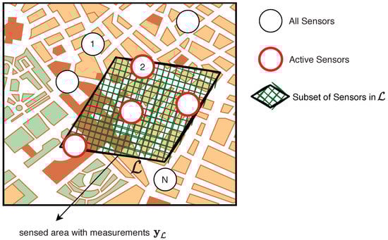
Figure 5.
General setup of the sensor placement problem. White circles represent all the N sensors. Circles with red contour denote the active sensors producing the measurement vector .
It is important to notice that the above optimization problem is combinatorial in nature, hence any brute force algorithm evaluating all the possible combinations would require an execution time that exponentially increases with the number of trial positions in , rendering the sensor placement problem impractical even for moderate values of N. To overcome such a drawback, alternative approaches that trade off the optimality of the obtained solution for a reduced complexity have been investigated in the literature. Some preliminary work has applied approximate greedy algorithms with the aim of directly minimizing the MSE. However, it has been found that MSE does not lend itself to being easily optimized due to the presence of several local minima. This called for the need of finding surrogate cost functions that tightly approximate the MSE while being much more efficient to optimize [75,297].
The methodologies used to solve (7) can be classified in three distinct groups:
- Greedy algorithms;
- Convex optimization;
- Heuristic strategies.
Greedy algorithms are appealing due to their polynomial complexity and the possibility to infer a certain degree of confidence about the solution’s quality by exploiting the submodularity of selected families of objective functions [298,299]. On the other hand, no guarantee in terms of actual MSE can be provided, and the optimization processes typically involve the inversion of very large matrices [300]. Convex optimization algorithms transform the original problem into a convex problem by relaxing the boolean constraints in (7) into a convex set [301,302]. Unfortunately, there is no easy way to establish the tightness of the relaxation and, consequently, to ensure the quality of the suboptimal solution. Furthermore, when the involved sensors should be distributed over a quite large area (e.g., in crowdsensing-based monitoring scenarios), efficient computational methods such as the alternating direction method of multipliers (ADMM) or the accelerated proximal gradient method (APGM) must be employed to speed up the sensor location process [303]. Heuristic approaches significantly lower the computational complexity required by the exhaustive combinatorial search but lack any kind of guarantee compared to convex and greedy approaches, both in terms of the optimality of the solutions and convergence [304,305]. Besides the approximation strategies, another important aspect concerns the nature of the physical field to be estimated. If can be assumed to be a spatio-temporally stationary stochastic process, as is the case for instance in flooding and long-term precipitation monitoring, more advanced approaches can be used to combine multiple snapshots using a proper deployment of fixed sensors that guarantee a cost-effective solution in terms of both processing time and energy [306,307]. On the other hand, if the physical field is assumed to be non-stationary, a condition experienced in crowdsensing and UAV-based environmental monitoring tasks due to sensor mobility, higher-order statistics need to be computed from multiple snapshots and included in the optimization problem to obtain a proper dynamic deployment of the sensors, so that the dynamics of the physical field can be accurately tracked [308]. There exist also low-complexity approaches that solve the optimal sensor location problem under some specific conditions. This happens, for instance, when the monitoring system is inherently distributed and the sensors are sparsely disseminated over large target areas (a condition typically found in crowdsensing-based monitoring). For these scenarios, sparsity can be enforced in the optimization problem and exploited to obtain more convenient, relaxed versions of the original cost function, leading to the so-called sparsity-aware sensor location methods [309,310]. Given their promising performance, such approaches have stimulated rich research activity in the last years [311].
5.2. Sampling and Reconstruction of Environmental Phenomena
One of the primary tasks performed by any environmental monitoring system is the accurate modeling of the specific natural phenomenon at hand, starting from a set of its samples. Prominent applications can be, for instance, the monitoring of water quality, for which suitable models able to predict the presence of pollutants need to be built. Typical samples may include the concentration of chemical pollutants or other related parameters such as the humidity, turbidity, or temperature. Other application fields are air quality monitoring in urban areas, analysis of the level of electromagnetic radiations, or the study of the soil moisture and related vegetation growth, just to name a few. In the signal processing literature, this process is known as spatio-temporal sampling and reconstruction of the specific physical phenomenon of interest. Thanks to the enhanced communication technologies available on sensor nodes, all the environmental data can be efficiently collected and further elaborated by centralized data processing algorithms, which leverage the link between the values of some selected environmental variables measured at specific locations and the position information itself to infer the behavior of the whole physical phenomenon, as shown in Figure 6. A physical phenomenon can be generally represented as a continuous function of two independent variables , with t denoting the time and the space variable (in either two or three dimensions). As discussed before, sensing nodes can only provide samples (or snapshots) of the continuous physical phenomenon collected at a finite number of locations and over a limited number of time instants , with , and T being the chosen sampling period. Questions that naturally arise are whether the discrete samples faithfully represent the physical phenomenon, and how the original function can be reconstructed from them, in either exact or approximate form. As an ubiquitous problem embracing several domains of the signal-processing literature, the process of reconstructing a physical field from a discrete set of its samples has received a lot of attention so far, and a number of different approaches have been investigated to solve it. The existing methodologies can be broadly classified in two main groups based on whether some a priori knowledge about the field is available or not. In the former case, more tailored approaches can be applied that benefit from the prior information (if e.g., admits a sparse representation or can be statically characterized according to a certain distribution) to achieve improved reconstruction performance. Conversely, in the latter case, the more classical tools from the sampling theory need to be adopted.
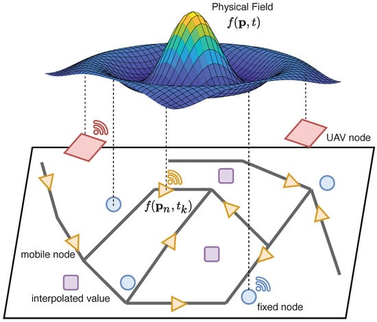
Figure 6.
Sampling and reconstruction of an environmental phenomenon . The WSN, UAV, and crowdsensing nodes measure the phenomenon at different physical locations. After reconstruction, the value of the field can be inferred also at unseen positions through interpolation.
5.2.1. Sampling and Reconstruction without Additional Information
The main results in terms of sampling and reconstruction root back to the celebrated Whittaker–Kotelnikov–Shannon (WKS) sampling theorem, which demonstrated that a physical field can be recovered with no errors if it is sampled regularly in the spatial domain with a sampling rate which is at least twice its bandwidth [312]. Clearly, the underlying assumption behind the theorem is that should have a limited bandwidth; unfortunately, this condition is hardly satisfied in practice, hence needs to be preliminarily filtered with a low-pass antialiasing filter. This operation intrinsically imposes that the field reconstructed from a limited set of filtered samples represents at most the optimal approximation of the original . Such a pioneering work has been then extended to more specific scenarios or multidimensional domains [313]. A more exhaustive analysis of regular sampling over multidimensional fields (also called lattices) has been conducted in [314], where authors were able to provide a closed-form expression of the MSE. With the aim of keeping the sampling and reconstruction process as general as possible, interesting approaches based on a probabilistic quantization framework have been devised, which only impose minor restrictions on the possible variations of some selected environmental variables [315]. Almost along the same lines, the authors of [316,317] presented very flexible pdf-unaware estimation approaches to reconstruct environmental fields having a homogeneous spatial distribution, able to operate also in the presence of very limited bandwidths.
In practical environmental monitoring applications, guaranteeing a regular distribution of sensor nodes (either fixed or mobile) over a target area is seldom possible and, more often, irregular sampling strategies need to be adopted [318]. The most important result in the field of sampling theory for nonuniform (but deterministic) sampling has been provided by Landau [319], who was able to derive the necessary density of samples that should be used to guarantee an exact reconstruction of the environmental field. In [320], further studies have been conducted to take into account realistic conditions such as the presence of errors on sensor positions and signals with non-limited bandwidth. It has been shown that theoretical insights can be obtained only when restricting to specific classes of possessing the shift-invariance property, and when linear interpolators are used to reconstruct the whole field.
A deterministic deployment of the sensor nodes (either regular or nonuniform) may not be possible when the monitoring system operates in hazardous or remote areas (as is the case in most natural disasters scenarios). In such contexts, sensors are randomly scattered over target areas (for instance, through airdrop) and their sampling process is inherently stochastic. If samples’ positions can be assumed to be realizations of a homogeneous Poisson point process (PPP), the MSE of the reconstructed field can still be analytically characterized under rather ideal conditions [321]. The effects due to realistic impairments such as quantization errors, energy constraints, and limited capacity further complicate the analyses, but some insights on the accuracy of the reconstruction process can be still extracted [322,323]. Recent studies have started to investigate possible extensions to the case of inhomogeneous sampling density [324], also considering stochastic sampling processes different from the PPP [325], so as to include additional aspects such as possible clustering effects [326] and the repulsion between points in the process [327]. An interesting comparison analysis between the deterministic and random sampling schemes has been conducted in [328], showing that the former provides improved reconstruction performance mainly in the high-SNR regime, while in the presence of low SNRs, both schemes behave in essentially the same way. A recent work explicitly analyzed the problem of reconstructing an environmental phenomenon from a set of samples randomly collected by crowdsensing vehicles [216]. By taking into account also the presence of a WSN infrastructure gathering data at fixed locations, it is demonstrated that stochastic sampling via crowdsensing leads to significantly improved reconstruction accuracy, especially when the WSN provides insufficient sampling information. Robust approaches able to infer environmental parameters from non-homogeneous and distribution-free data opportunistically gathered by crowdsensing nodes have also been considered [329].
The increasing availability of large unstructured datasets containing several different environmental data is stimulating the adoption of fully data-driven approaches to infer the behavior of environmental phenomena. A preliminary work tried to represent such “big environmental data” using the theory of graph signal processing [330]. An exploratory analysis has been conducted in [331] for the specific case of urban air pollution data, showing how the latter could be represented as a high-dimensional and geometrically structured graph signal. The analysis has been conducted on a real dataset of PM2.5 and NO measurements from New York City, and the results demonstrated that interesting information such as the identification of the most polluted areas could be readily inferred. This pioneering work opened up a promising research direction in which methods from the emerging field of graph signal processing can be used to analyze the complex dynamics of environmental phenomena [332,333].
5.2.2. Sampling and Reconstruction with a Priori Information
When additional information on the physical field is available, more tailored sampling and reconstruction approaches can be used to further lower the number of required samples.
Deterministic A Priori Information: In some more controlled environments, it is possible to gain a better understanding of the physical phenomenon and establish deterministic (either physical or chemical) laws that accurately relate the involved environmental variables in time and/or spatial domains. An environmental monitoring system can be viewed as a set of heterogeneous sensors measuring different environmental variables. Let us denote with the M different environmental variables measured by the sensors, where we considered the 1D case only to ease the notation. Assuming that represent different manifestations of the same environmental phenomenon , they can be linked through some underlying analytical relationship. For instance, if the behavior of the functions can be linked via a system of linear differential equations with constant coefficients, describing the physical correlations among them, an additional constraint can be exploited in the reconstruction process
where denotes the Fourier transform of the m-th function and is a known matrix, with P number of differential equations in the linear system. Interestingly, if we assume that the functions have a limited bandwidth in the interval , but sensors are able to gather measurements only at a fraction of the corresponding Nyquist sampling rate , with denoting the undersampling factor, a perfect reconstruction of the original functions is still guaranteed if [334]
The inequality in (9) conveys a rather important message: being that the upper bound is an increasing function of P, which we recall is the number of equations describing the physical model in (8), the more prior information about the environmental phenomenon is available, the less samples are required to perfectly reconstruct it.
A number of papers investigated different declinations of such a general framework to tackle more specific environmental monitoring problems, based on the availability of suitable physical models. For instance, the authors of [335] considered an array of chemical sensors and proposed novel algorithms to detect and localize potential sources of polluting vapors based on a generalized likelihood ratio test (GLRT). Flick’s law of diffusion has been used to model the pollutants released by a single source, emitted with a constant rate and starting from an unknown time instant. The same idea has been then extended to the case in which the chemical sensors are moving instead of fixed [336] and to more general air and ground scenarios [337]. To accurately model the diffusion of chemical pollutants in arbitrary 2D environments, a finite-element (FE) method has been integrated in [338] to linearize the spatial and temporal derivatives of the original differential equations. In addition to the detection and estimation of a biochemical source, the space–time pollutant concentration diffusion and its future evolution have been estimated in [339] using a maximum likelihood algorithm, taking as reference scenarios a propagation through two different semi-infinite mediums. With the aim of representing realistic scenarios while keeping the required computational complexity tractable, in [340] the biochemical dispersion model considered so far has been suitably approximated using a Monte Carlo numerical approach, which decoupled the fluid simulation from the transportation phenomena using a Feynman–Kac representation. The obtained model was general enough to emulate additional random effects such as chemical reactions, temperature effects, and radioactive decaying. A Bayesian framework has been considered to solve the associated inverse problem and retrieve the position of the polluting source. Similarly, in [341] the same approximated physical model has been coupled with a sequential change detection approach to promptly identify the time of release of biochemical pollutants. The authors of [342] addressed the problem of sampling and reconstructing the time-varying atmospheric emissions produced by industrial smokestacks. The physical phenomenon has been modeled using a set of partial differential equations (PDE), and sufficient conditions to estimate the emission rates were provided. In [343], the Fukushima disaster that occurred in 2011 was investigated using the above framework, with the aim of inferring the amount of radioactive material released and its consequences. The proposed method leverages sparse regularization to solve the problem and estimate the plausible amount of released Xenon, using an atmospheric dispersion model to emulate the radioactive emission process.
Stochastic A Priori Information: Although the deterministic modeling approach may be suitable for some specific and controllable environmental contexts, it cannot be easily applied in the presence of more complex phenomena. For instance, the air pollution in a crowded urban area is linked to several unpredictable factors such as the traffic density, the weather conditions, the specific type and configuration of the buildings, just to name a few. For these contexts, finding an appropriate physical model able to correctly capture all the involved variables and their interdependencies is a very challenging task, if not impossible. Stochastic processes represent an elegant way to overcome the lack of a physical model, as they allow a more general representation of an environmental phenomena through the use of regression or interpolation techniques, operating on all the measured data. A specific class used in most environmental contexts is that of Gaussian Processes (GPs), which are powerful tools for non-parametric regression able to provide an estimate of the field together with a measure of the corresponding uncertainty [344].
To simplify the exposition, we omit the time variations of the physical phenomenon and consider the sole dependency on the position , thus obtaining a spatial field . The spatial field is sampled by a set of N sensors located over the target area at known positions , with each observation expressed as
where represents the (additive) measurement noise component modeled as an i.i.d. Gaussian random variable with zero mean and variance . (It is worth noting that each sensor n can perform multiple measurements of the spatial field, say . Without loss of generality, we consider the case of .) The reconstruction process then consists in using the set of measurements and associated positions to estimate the value of the unknown spatial field at a set of regression positions . In principle, a regression position could either coincide with a measurement position or not. Using the common terminology of machine learning, in the former case we refer to such points as training points, in which sensors aim at improving their local estimate of . Conversely, in the latter case they are called testing points, and the corresponding estimates of are the interpolation (or prediction) of the spatial field at new unseen points of the space. If the spatial field admits a parameterization in terms of a finite set of hyperparameters , the latter can be inferred from the measurements set by using parametric regression techniques. As anticipated, in more complex environmental monitoring tasks, no exact or accurate parametric models for are available. A more convenient way to handle such contexts is to assume that the spatial field is a sample from a GP
with mean function and covariance function . Customary covariance functions, also called kernel functions, include the Matern functions, the squared exponential functions, and the neural network functions, among many others. In other words, a GP imposes a multivariate Gaussian distribution over the space of functions that maps the sampling locations to the corresponding noisy measurements. It is not difficult to show that, since the joint distribution of the spatial field values measured at the training and test locations is Gaussian, so is the conditional distribution of at a generic test position , given the measurements at the training positions . Therefore, given , it is possible to infer the distribution of the spatial field at a given test location as
where the conditional mean and variance are given by
with denoting the expectation operator, the identity matrix, an dimensional vector whose n-th entry is the cross-covariance between the test location and the n-th training location, and the covariance matrix of the training locations whose -th element is given by , with .
The probabilistic framework in (13) allows us to reconstruct an estimate of the overall spatial field by optimally combining all the measurements gathered by sensors in the monitoring system. Despite its elegant formulation, there are a number of aspects that need to be considered and some issues that should be carefully handled. For instance, the inversion of the Gram matrix appearing in (13) can become computationally demanding as the number of sensors N increases. To overcome such a drawback, some works have proposed to approximate the Gram matrix with lower dimensional matrices acting as surrogates [345], or to exploit the possible regular displacement of sensors to implement a fast matrix inversion based on FFT approaches [346]. Other approaches have investigated the possibility of converting the covariance functions into infinite-dimensional stochastic differential equations [347]. In doing so, an approximation of the covariance function can be obtained in terms of an infinite-dimensional state-space model, where each element of the state coincides with a different order derivative of the original GP. As the solution of this approximate representation is a Markovian process, more efficient approaches such as the Kalman filter or its variants, possibly combined with a smoother one such as the Rauch–Tung–Striebel, can be used to compute the predictive distribution in (13) with a reduced (linear) complexity [348]. To cope with the more challenging case of large-scale monitoring based on crowdsensing, where the number of involved sensing nodes can be significantly higher, a suitably designed combination of GP and state-space models has been recently proposed in [349]. Interestingly, the proposed resolution method allows to compute (13) with a complexity that does not increase with the number of sensors N.
Besides computational aspects, a plethora of work has been devoted to the use of GP processes for environmental field estimation. For instance, the authors of [350] proposed a general modeling approach based on the Gaussian Markov random field, a specific category of GP, with the aim of inferring the behavior of a number of non-stationary environmental phenomena. An algorithm called the spatial best linear unbiased estimator has been derived in [351] to estimate standard spatial Gaussian fields, taking into account also the presence of non-idealities such as observation and quantization errors due to communications over the wireless channel. To infer information about environmental phenomena modeled by time-varying spatial GPs, a low-complexity regression method is presented in [352], which exploits only a limited set of measurements collected by a set of mobile sensor nodes (either terrestrial or aerial) with limited processing and storage capabilities. A Bayesian estimation framework has been applied in [353] to design algorithms able to compute the predictive distributions in (13) with a constant computation time, irrespective of the total number of measurements to be processed. In [354], a flexible generalization of a GP is proposed to estimate a spatial field by means of an empirical Bayes approach. Specifically, the main idea is to express the mean function of the GP by means of general parametric equations. Such a reparameterization can be used to encode any a priori knowledge of the physics generating the spatial field, as well as any data-driven information. The authors of [355] framed the GP regression problem under an extended Bayesian optimization framework and solved the additional problem of accurately choosing the best measurement locations that maximize the regression accuracy while taking into account the distance traveled by mobile sensor nodes.
The average number of samples required to correctly infer the behavior of an environmental field can be further lowered if it admits a sparse representation on some basis [356]. In these contexts, compressed sensing techniques operating on infinite-dimensional and time-varying vectors represent a useful tool to guarantee a reconstruction up to a limited error in terms of MSE [357,358]. Although promising, such techniques are based on the underlying assumption that the environmental phenomenon possesses the SI property, or at least belongs to a space of generalized SI signals (combination of SI subspaces) [359]. Moreover, having a basis function representation for an environmental phenomenon means that the latter can be constrained to lie in a space having a fixed topology, which may not be often the case [360]. For the specific case of crowdsensing or UAV-based monitoring, distributed compressive sensing techniques can be employed to further lower the complexity of the reconstruction process by leveraging spatial and temporal correlations among data [361,362] and also when processing vectors of heterogeneous environmental measurements [220].
5.3. Environmental Monitoring Based on Hyperspectral Image and Signal Processing
Over the past decades, hyperspectral imaging has been affirmed as one of the leading technologies for a variety of environmental monitoring applications in different marine, land, and aerial contexts. Initially developed for remote sensing applications based on satellite and airborne systems, hyperspectral imaging has nowadays reached an unprecedented level of spatial, temporal, and spectral resolution, opening the door for new environmental monitoring applications requiring a very fine and detailed analysis of materials and their physical properties. Thanks to the rapid evolution of integrated sensor technologies, lightweight hyperspectral cameras can be easily carried by UAV platforms. Some new exciting applications of hyperspectral sensors recently appeared also in the field of smartphone-based environmental monitoring. This emerging topic, known as smartphone spectroscopy, has the ambition of making most of the powerful features of hyperspectral imaging available also in our compact handheld devices [363,364]. Handling such an increasing number of environmental applications calls for advanced signal processing algorithms able to cope with the complex process of extracting relevant information from hyperspectral data [365]. Very high dimensionality, spectral mixing effects (either linear or nonlinear), and a rather complex measurement process are only few examples of the several challenges behind the hyperspectral technology [366]. The theoretical tools used to deal with such issues span different fields, from image and signal processing to statistical inference and even the more recent machine learning and deep learning techniques.
5.3.1. Hyperspectral Image Acquisition and Representation
In a nutshell, hyperspectral sensors aim at measuring the electromagnetic reflection, absorption and emission characteristics of a given material and to classify it based on its chemical and physical composition. The basic principle consists in acquiring the radiation generated by each object, represented by a set of pixels in a given scene, over a spectrum of different frequencies (i.e., different wavelengths). Collecting tens or hundreds of spectral channels allows to construct a spectral signature of the object of interest, which can be then used to recognize the nature of its constituent materials. Commercial hyperspectral cameras acquire data over a portion of the electromagnetic spectrum ranging from the visible region (from to m) to the short-wave (below m) and mid-wave infrared regions (below 5 m), and even up to the long-wave infrared region (below 14 m), with a sampling step between 6 and 10 nm. Given its three-dimensional nature, a hyperspectral image is usually referred to as hyperspectral data cube or hypercube and can be mathematically defined as a tensor , with H and W denoting the spatial size of the data and d the number of spectral channels (or bands). Notice that, due to the high spectral sampling frequency, all the d channels are highly correlated and the useful spectral information typically resides in a lower-dimensional manifold of the spectrum. The hypercube is typically unfolded in two alternative ways before processing:
- As a set of vectors in the spectral dimension , , with each representative of the j-th pixel in the image.
- As a set of matrices in the spatial dimension , , with each a grey scale image containing all the pixels at the i-th spectral band.
The first representation is useful when the different objects in the scene can be better separated in the spectral domain, owing to the principle that similar materials likely share similar spectral vectors . Conversely, the second representation is more adequate when the objects’ similarities are more evident in the spatial dimension; hence, neighboring pixels can be clustered based on their correlations and different materials can be easily recognized through image segmentation techniques. We report a pictorial example of a hyperspectral image and its possible representations in Figure 7. The literature on hyperspectral imaging and signal processing is quite vast and covers a lot of different topics. In the following, we review three main categories of processing techniques, namely classification, spectral unmixing, and change detection, which are more frequently used in the environmental monitoring literature. We refer the interested reader to [367,368,369] and to the references therein for a more comprehensive overview of hyperspectral data analysis techniques.
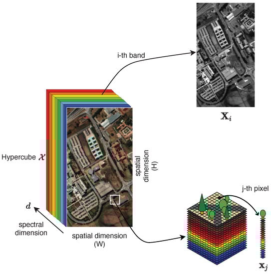
Figure 7.
Two alternative unfoldings of the hypercube along the spatial or spectral dimensions.
5.3.2. Hyperspectral Image Classification
Hyperspectral image classification is among the most active areas of research in the field of environmental monitoring [370]. An uncountable number of monitoring tasks including the identification of industrial discharges (solid and liquid residues, radioactive waste, gas emissions), the littering on coastal and sea surfaces, the outbreaking of wildfires, and many other land degradation phenomena can be accomplished by using hyperspectral classification algorithms. Given an observed hypercube , the main goal of a classification algorithm is to associate each spectral vector with a specific class (or label) that identifies its nature. Individual classes or labels should try to uniquely represent a given type of material or land cover (e.g., distinguishing trees from soil, streets and buildings) and are usually defined by specifying some kind of similarity measure in the considered feature space [371]. Therefore, classification techniques are based on the underlying assumption that the spatial resolution of hyperspectral sensors is high enough to guarantee that each pixel in the image is characterized by a single dominant spectral signature (called pure pixels). When, conversely, images contain pixels whose spectral signatures are a mix of different components, spectral unmixing approaches need to be adopted, as will be discussed in the next section. Two subsequent steps are typically involved in the classification of a hyperspectral image:
- First, a dimensionality reduction is performed on the hypercube to remove the redundant spectral information and keep only the most informative components, thus avoiding the curse of dimensionality and, at the same time, preserving the limited storage space available on UAV platforms [372].
- In a second step, a specific classifier is trained based on a chosen design strategy and used to label each spectral vector.
The dimensionality reduction step includes a feature selection and a feature extraction phase [373]. Given a set of initial features , feature selection aims at retaining only a small subset of them, denoted by , according to a suitable criterion that tries to preserve the classification performance, with and [374]. On the other hand, the feature extraction phase aims at finding a suitable linear or nonlinear transformation that maps each higher-dimensional spectral vector into a corresponding reduced D-dimensional vector , , while trying to preserve the maximum amount of initial information in this new reduced feature space [375]. Based on whether it is possible to label each individual class or not, dimensionality reduction methods can be grouped into supervised, semi-supervised, and unsupervised approaches. Examples of supervised methods are the linear discriminant analysis (LDA) [376], the nonparametric weighted feature extraction (NWFE) [377], the mutual information [378], and their variants. Semi-supervised methods, used when only a very limited number of labels are available, include graph-based learning [379], cotraining [380], and transductive SVM [381], while common unsupervised methods are principal component analysis (PCA) [382], independent component analysis (ICA) [383], minimum noise fraction (MNF) [384], and their nonlinear versions.
The design of a specific classifier in the second step is conducted considering either spectral-only information or by jointly exploiting spectral and spatial dependencies. To simplify the design, approaches in the former group neglect the spatial correlations existing among pixels and treat the hypercube as a set of independent spectral vectors . As the identification of potential environmental risks (e.g., illegal landfills, abusive buildings) typically triggers a chain of legal and prosecutorial actions, an accurate classification of objects appearing in the scene is of utmost importance. This makes supervised spectral approaches largely preferable over both semi-supervised and unsupervised ones for environmental tasks. Unfortunately, in practical scenarios, the amount of training samples is often insufficient to allow a satisfactory training of supervised classifiers. Thus, handling high-dimensional data using only a limited amount of training samples represents one of the main challenges in the classification of environmental hyperspectral images. In addition to more traditional supervised approaches (e.g., SVM, random forest, back-propagation neural networks) [385], deep learning methods are also emerging as valid tools to learn high-level features that are inherently more robust against the non-idealities of hyperspectral images [386,387].
Considering that objects appearing in an environmental scene are usually larger than the dimension of a single pixel, neighboring pixels are inherently correlated in the spatial dimension. Such correlations provide additional information on the shape of the objects and can be thus fused with the spectral information to obtain improved classification performance [371]. Two main strategies can be adopted to infer the spatial information in the hypercube: a first family of approaches, called crisp neighborhood, extracts spatial information by considering only a restricted number of adjacent pixels and using a probabilistic model (such as the Markov random fields) to describe correlations as a two-dimensional stochastic process defined over a lattice of discrete points [388]. The second family of approaches, known as adaptive neighborhood, tries to extend the number of involved pixels by using image segmentation algorithms [389]. The spatial and spectral information are then fused by using composite kernel functions such as the generalized composite kernel (GCK) [390] or multiple-kernel learning [391].
Irrespective of whether spectral-only or combined spatial–spectral information is used for classification purposes, from the surveyed literature we can conclude that a general classifier that can be seamlessly used in all the diverse environmental contexts and still provide the best performance in terms of accuracy does not exist. To be effective, a hyperspectral image classifier should be designed by explicitly taking into account the different training and testing data at hand, integrating whenever possible also some a priori knowledge of the considered application domain.
5.3.3. Hyperspectral Unmixing
The classification methods reviewed so far assumed that each spectral vector is characterized by a single dominant spectral signature. In realistic acquisition scenarios, sensing nodes (e.g., UAV platforms) are subject to a number of mechanical effects (e.g., vibrations, wind, adverse atmospheric conditions, and other effects related to the dynamics) that cause a destabilization of the hyperspectral sensor. As a consequence, the spectral content of pixels in the recorded hypercube could be a mixture of radiations generated by many materials appearing at the same location covered by each pixel. Mixing effects can be also experienced when the hyperspectral sensor is perfectly stabilized but its spatial resolution is so high that intimate mixing phenomena spuriously appear. The latter case explains the well-known trade-off between spatial and spectral resolution in hyperspectral imaging. In all these cases, it is no longer possible to use the spectral signature of each pixel as discriminant to infer information about the materials present in the scene. To overcome such issues and restore the high classification performance obtained in the case of pure pixels, hyperspectral unmixing algorithms, also called blind source separation methods, need to be adopted. Basically, they try to exploit the rich spectral resolution intrinsinc in to unmix the spectral contents of each pixel.
Hyperspectral unmixing has been widely investigated in the literature, and a number of methods have been proposed to mitigate or completely remove mixing effects under different operating conditions [392,393]. In the more specific environmental monitoring contexts, linear mixture models (LMMs) gained more attention due to their simplicity and mathematical tractability. Such models assume that mixing effects occur at a macroscopic scale and that each radiated signal is associated to a single material in the scene. The radiations emitted by the materials are therefore almost separated but, due to the limited spatial resolution of the hyperspectral sensor, appear as linearly superimposed in the recorded hypercube . This is tantamount to modeling each measured spectral vector as the sum of P different spectral contributions as
with denoting the spectral signature of the p-th material, known as endmember, while quantifies the percentage of the p-th material in the j-th pixel, known as fractional abundance. Being that s are fractional values, they satisfy the abundance non-negativity constraint , and their individual values are constrained by (abundance sum constraint). Based on (14), the hyperspectral unmixing problem can be then recast as the problem of estimating the P endmembers and their associated fractional abundances , for each . Denote with the matrix of hyperspectral data obtained by arranging all the spectral vectors in columns and, similarly, with the matrix containing all the endmember vectors . Defining as the abundance matrix whose columns are the fractional abundance vectors of each pixel , the linear hyspectral unmixing problem can be thus formulated as
where is the Frobenius norm operator and, with a slight abuse of notation, the abundance non-negativity constraint should be intended in an elementwise fashion. Notice that (15) admits a double interpretation in terms of matrix factorization or, alternatively, as a linear blind source separation problem [394]. The main linear unmixing strategies used to handle hyperspectral environmental data can be broadly grouped in two categories based on whether endmembers are assumed to include pure pixels—for which sparsity or geometry-based approaches can be considered [395]—or, conversely, some of the endmembers are assumed to be missing in some pixels, using in those cases volume-based approaches [396,397]. In the presence of highly mixed data, however, both the previous approaches tend to fail, and the unmixing problem needs to be solved under a statistical framework [398], possibly considering the additional use of spatial information to complement the spectral one [399]. Other related research problems include the estimation of the actual number of endmembers P [400] and the characterization of their space-time variations [401], also including the extension to non-linear mixing models [368].
5.3.4. Hyperspectral Change Detection
Besides classifying the different materials present in a target area at a given time instant, hyperspectral imaging can be used to support the continuous monitoring of a geographical surface, with the aim of promptly detecting significant changes that can occur over time [402]. In most environmental contexts, such changes could be indicative of man-made actions (either intentional or accidental) or potential natural disasters that may compromise environmental health [403]. To formally define the change detection problem, let us assume the availability of two hyperspectral cubes and capturing the same geographical area at two different time instants and , respectively. By computing the hyperdimensional difference pixel by pixel, we obtain a new image
encoding the spatial and spectral changes that occurred in that particular area. Assume that is the set of all possible classes in the difference image , with being the no-change class and being the set of K classes representing the different types of changes that can occur. Then, the task of identifying a significant change can be formulated as either a binary or a multiclass change detection problem. In the former case, the process aims at separating the no-change hypothesis from any possibly changed hypothesis in , with no distinction within the latter set [404]. Conversely, in the latter case, the goal is to identify pixels with substantial changes in and to recognize the specific classes in that they belong to [405]. The general process of detecting changes in the difference image is typically split in two main steps.
Anomaly Detection: First, an anomaly detection process is conducted over the whole image with the aim of identifying pixels whose spectral variations are significant in magnitude (or according to other metrics) with respect to the other adjacent pixels representing the background [406,407]. Compared to more traditional optical images, where abrupt changes tend to emerge frequently, in hyperspectral imaging changes are intrinsically more implicit and complex, calling for advanced change-detection methods able to capture even very subtle variations that do not easily stand out from the background [408]. In this first processing step, targets of interest are not yet outlined and anomaly detection is conducted without any a priori spectral information. The Reed-Xiaoli (RX) detector represents one of the most effective algorithms to identify anomalies in a huge variety of environmental hyperspectral data. It was derived from the GLRT under the conservative assumptions of targets with unknown spectral distribution, embedded in background clutter with unknown spectral covariance. Denoting with a generic spectral vector extracted from the difference image , to be tested against a possible anomaly, the RX algorithm consists in the following test [409]
where and denote the estimated mean vector and covariance matrix of the background clutter, respectively, and is a threshold to be set according to the desired probability of false alarm. Both and can be estimated globally on the whole hyperspectral image, using a multivariate Gaussian distribution to model the background clutter [410], resorting to linear subspaces [411], or through segmentation techniques inherited from optical image processing [412,413]. Alternatively, local estimation approaches based on sliding circular windows centered around a given pixel have been considered to obtain more accurate estimates of the background clutter, especially when some portion of can be excluded upfront [414]. In addition, several variations of the RX algorithm have been devised in the literature to achieve improved detection performance with possibly reduced false alarm rates [409,415].
Target Detection: In a second step, the identified anomalies are further verified through target detection methods to establish whether their spectral signatures can be associated to a target of interest (e.g., a pollutant material) or should be instead attributed to spurious variations caused by the natural clutter. Target detection methods leverage some a priori knowledge about the desired targets to infer their possible presence. Specifically, in the environmental monitoring literature, target materials are usually characterized by either a single spectral signature [416] or by specifying a signal subspace they belong to [417]. In the former case, the GLRT detector is the so-called spectral matched filter (SMF), whose decision statistic for a spectral vector under test is computed as [418]
where is the known target spectral signature and is the estimated clutter covariance matrix. The SMF detector is derived by assuming that the background clutter follows a zero-mean Gaussian distribution ; the target is also Gaussian-distributed and shares the same statistics of the clutter but has a generally non-zero mean , with the abundance factor encoding how strong the target presence is inside the pixel vector . To overcome possible numerical issues arising in the computation of the decision statistic (18), the SMF detector can be modified by discarding eigenvectors whose associated eigenvalues fall below a predefined noise threshold [419], or by adding a regularization factor to before its inversion [420].
When both target and natural clutter spectral signatures can be assumed to belong to two separated linear subspaces, the GLRT detector is represented by the subspace matched detector (MSD), having the following decision statistic
where and represent the projection matrices onto the clutter-only and target plus clutter subspaces, respectively. By elaborating on the same idea, alternative detectors such as the adaptive subspace detector (ASD) [421] and the orthogonal subspace projection (OSP) [422] have been proposed in the literature. These three detectors are still considered the benchmarks for target detection in hyperspectral imaging.
6. Integrated Large-Scale Air–Ground Environmental Monitoring
The review of the individual WSN, UAV, and crowdsensing technologies outlined that, despite remarkable improvements in some specific application contexts compared to the use of legacy systems, the monitoring capabilities for most approaches proposed in the literature are still limited by either the insufficient information gathered by sensor nodes (incomplete or inaccurate) or by some intrinsic limitations of the adopted technologies (e.g., limited sensor autonomy, restricted operating areas). Nonetheless, the rapid impact of environmental changes on both the economy and health of the modern society signals the need for advanced monitoring systems able to operate on large geographical scales, and to provide integrated (air, land, sea) real-time and long-term analyses from a big amount of heterogeneous environmental data. A possible way to meet such requirements is to consider the design of hybrid monitoring systems that try to combine the benefits of more technologies.
6.1. Hybrid Environmental Monitoring Systems
A first step toward this idea is, for instance, the hybridization between the ground sensors of a WSN and the aerial UAV nodes, a topic that has started to attract attention in the environmental research community [52,423]. Complementing a fixed WSN with UAV nodes brings three main advantages: (i) a more extended and finer monitoring of the target area becomes possible thanks to the aerial inspection capabilities of UAVs, which enable a more focused and controlled analysis of the environmental phenomena, reducing the risk of losing potentially critical data; (ii) a better management of the energy consumption can be achieved by designing suitable interplay sensing strategies between WSN and UAV nodes which, by extending the autonomy of each individual sensor (either fixed or mobile), can prolong the whole system lifetime and ensure a long-term monitoring of the area of interest [424]; (iii) an increased flexibility of the monitoring system is obtained thanks to the versatility of UAV nodes, which can be easily converted to mobile base stations and used to extend the communication range between the WSN and the monitoring centers, or even used to support the physical deployment of WSN nodes [425]. When applied to the fields of air pollution or radioactivity monitoring, a hybrid WSN-UAV system can leverage its three-dimensional inspection capability to provide a much more accurate prediction of the propagation and evolution of pollutants over time [426,427], allowing a better assessment of their potential impact over a large geographical scale [428]. Hybrid WSN-UAV systems can also bridge the gaps existing in marine applications, where access to WSN nodes disseminated over the sea surface is often very difficult, or almost impractical in cases of underwater deployments [429]. In such contexts, the WSN can be employed for data collection (e.g., temperature, humidity, turbidity), while UAVs mainly act as aerial sinks for the periodic offloading of such data. An experimental test conducted in [430] demonstrated that, remarkably, a collaborative WSN-UAV monitoring system can achieve an extended operating range of about 5 km from the coast, while guaranteeing a bit rate of about 10 kbps. WSN and UAVs can actively cooperate to support authorities in the presence of natural disasters, from the initial provisioning phase up to disaster recovery [431]. Since disaster management applications usually operate in harsh environments, UAV nodes can be employed for a preliminary scanning of the target area, with the aim of identifying the best candidate zones to perform aerial and ground measurements [432]. Then, in a second step, WSN nodes equipped with proper sensing units are deployed and used to carry out more detailed measurements [433]. A key advantage of a hybrid WSN-UAV system is its capability to dynamically readapt to the priorities of the disaster scenario at hand, either in terms of safeguarding human lives or providing real-time analyses based on the intelligent fusion of all the available environmental data [53].
Almost along the same line, some recent work has started to consider a combination of WSN and crowdsensing as well as a combination of crowdsensing and UAV technologies. The former systems aim at increasing the too-coarse sampling capability of WSNs by integrating measurements opportunistically gathered by mobile crowdsensing nodes on a denser scale. From a spatio-temporal perspective, the two technologies reinforce each other: mobile crowdsensing can be largely exploited during the daytime, when citizens carry out their daily activities. In the meantime, WSN nodes can be set in sleep mode to preserve their energy. Conversely, during the night time, when the number of crowdsensing nodes is typically scarce, the hybrid system can schedule WSN nodes to perform data collection. Hybrid WSN-crowdsensing monitoring systems have found some applications in the field of air quality monitoring to face the significant spatial variability of particulate matters [54,434]. A prototype system based on low-cost, off-the-shelf hardware mounted on both fixed (WSN) and mobile (crowdsensing) nodes has been recently developed in [435]. Preliminary results from six months of data demonstrated that the system can reliably reveal areas with exceeding levels of PM2.5 and PM10 and, interestingly, can guarantee a high sampling rate of about one measurement per second. Similarly, hybrid crowdsensing–UAV monitoring systems have been conceived with the idea of broadening the sensing horizon of mobile crowdsensing nodes, especially when operating in areas that could be hardly reached by terrestrial vehicles (e.g., flooded areas, forest areas) [436,437]. Additionally, in this case, the few available prototypes of collaborative crowdsensing–UAV systems have been mainly employed for air-quality monitoring [438], also considering the reuse of UAV platforms dedicated to package delivery [439].
6.2. Combining WSN/UAV/Crowdsensing and Advanced Signal Processing
Despite that significant work has been devoted to the application of each specific technology to the diverse environmental contexts, as illustrated in Section 2, Section 3 and Section 4, the interlinking between different types of technologies has only recently appeared in the literature and its potential has not yet been fully explored. More specifically, most of the hybrid systems discussed in Section 6.1 are often restricted to quite limited areas and are intended only for a few specific types of analysis (e.g., only marine pollution or only air pollution). Furthermore, the design approaches mainly focus on aspects related to the degree of reactivity of the monitoring system, i.e., the ability of the proposed system to respond promptly to the occurrence of critical events such as, for instance, large wildfires or spills of pollutants into the sea. However, less attention has been devoted to the possibility of using, in a complementary way, proactive approaches that allow for identifying potential high-risk areas and to implement preventive actions in advance, aimed at reducing the probability of events with a high environmental impact. Overall, none of the available systems is able to ensure an integrated monitoring of the environment in all its aspects (air, land, and water), while offering a cost-effective and scalable solution to support a large-scale coverage. In this respect, we believe that the integration of the three different monitoring technologies (WSN/UAV/Crowdsensing), coupled with the use of advanced signal processing techniques such as those presented in Section 5, will be at the basis of future monitoring systems, igniting a new era of ubiquitous environmental monitoring.
In Figure 8, we depict the main application contexts of a unified framework for integrated large-scale environmental monitoring, with the aim of illustrating tasks for which a combined use of air–ground technologies is possible, and those for which WSN, crowdsensing, and UAV are alternative or complementary. More specifically, scenario (A) represents a typical urban environment characterized by the presence of several potential sources of pollution: on the one hand, there are a number of electromagnetic sources such as antennas installed on the roofs and mobile devices transmitting in the area; on the other hand, a number of vehicles passing through the intersection may contribute to the potential increase in air pollution levels (due to engine exhausts) and noise pollution levels due to engine noise (e.g., heavy traffic, motorbikes, and large cars) or an improper use of horns. In this application context, a set of mobile devices recruited as crowdsensing nodes provides important real-time information related to some key environmental parameters. This information can be processed through advanced signal processing algorithms (such as those discussed in Section 5) to constantly monitor the spectrum of radio and acoustic frequencies, quantifying the energy content of the detected signals and assessing the consequent impact on the environment. By combining this information with that deriving from the analysis of vehicle emissions, it is also possible to infer useful information to support applications for traffic control and road safety (e.g., to avoid frequent congestion on the main city backbones and to reduce the number of accidents). Scenario (B) is representative of a case of soil pollution caused by the illegal dumping of solid waste. In this case, one or more UAVs can be used to acquire images/videos and data from hyperspectral sensors. Such data can processed through hyperspectral signal processing techniques (see Section 5.3) to analyze the physical characteristics of the different materials and classify them according to their spectral signatures. Subsequently, the optical data can be used to validate and confirm the actual presence of waste in the surveyed area. Scenario (C) illustrates a case in which some industrial waste may have spilled into the soil. In order to cope with this scenario, the air–ground framework combines the use of UAV nodes with the sensing capabilities of a WSN. The latter, in fact, thanks to the availability of sensors dedicated to the analysis of chemical and biological substances, is able to identify any contamination of the subsoil that could not otherwise be revealed through the data acquired by UAVs. Similarly, scenario (D) relates to the emission of industrial smokes and can be addressed through the joint use of WSN and UAV nodes, and it is further enhanced by including the contribution from citizens. Specifically, air pollution measurements gathered by WSN nodes can be exploited to determine if the maximum tolerable thresholds in the area have been exceeded. When this happens, WSN data will be integrated with the optical and hyperspectral data acquired by the UAVs to locate the pollutant source, using information from crowdsensing nodes (e.g., photos) to support the identification process. Scenario (E) illustrates a typical case of forest fire, for which the sensing capabilities of a fleet of UAVs play a key role. On the one hand, the processing of hyperspectral data allows the early detection of a fire outbreak. In the event that a potential fire is identified, if the UAV nodes are also equipped with LIDAR sensors, these can be used to verify the correctness of the triggered event, thus reducing the number of false alarms and saving important emergency response resources. In addition to fire detection (reactive approach), data from optical and hyperspectral sensors can be combined with measurements from thermal sensors to identify high-risk areas (proactive approach). For instance, areas with a high density of dry vegetation and high temperatures may be subject to preventive actions aimed at avoiding the outbreak of fires. Scenario (F) represents a typical marine environment. In this context, a WSN can be deployed on the shore and/or on appropriate buoys located at strategic points of the sea. By fusing information from pressure, thermal, and biological sensors, it is possible to monitor important parameters (e.g., water turbidity level, presence of biological indicators) in real time. Moreover, the possible presence of pollutant spills in the sea shown in scenario (G) can be revealed by processing, in addition to the data from WSN nodes and acquired by UAVs as well as the explicit feedback coming from citizens. Overall, it is evident that the three air–ground monitoring technologies (WSN/UAV/crowdsensing) can be used in a synergistic manner to compensate for the limitations of each individual technology, motivating their joint use in future integrated and large-scale monitoring systems.
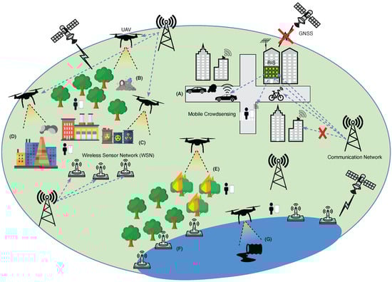
Figure 8.
Overview of potential uses of WSN, UAV, and crowdsensing inspection capabilities to enable integrated and large-scale environmental monitoring.
The idea of creating a collaborative system made of fixed and mobile terrestrial nodes, as well as of aerial UAV platforms, is indeed not new. In recent years, we have been witnessing an impressive growth in the number of smart devices and services that need to be supported by existing communication networks. To fully manage the ever-increasing data demands generated by the several heterogeneous applications emerging under the IoT umbrella, architectures at the basis of next-generation 5G and beyond (6G) communication networks will integrate satellite, aerial, and terrestrial communications under the so-called space–air–ground network paradigm [440,441,442]. It is thus natural to look at environmental monitoring as a big and complex service that can be supported by such emerging architectures. For instance, in [443], it was shown that a combination of smartphones, sensors, and UAVs can effectively overcome the limitations of an unstable communication environment in the presence of a natural disaster. However, several other aspects besides communication should be taken into account to treat the topic in its entirety. Indeed, the considerable complexity of ensuring integrated large-scale environmental monitoring is also related to the great diversity among the air, land, and water contexts, to the huge variety of sensing platforms carrying heterogeneous sensors, and more generally to the specific characteristics of each individual monitoring task. In Figure 9, we identify the main components of a high-level architecture that leverage the different sensing capabilities available on the three levels made up of WSNs, crowdsensing, and UAVs, to enable large-scale integrated monitoring (atmospheric, marine, acoustic, electromagnetic, and soil) of the environment.
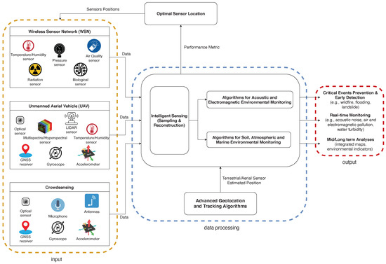
Figure 9.
Main components of the proposed three-level monitoring architecture combining WSN/UAV/crowdsensing technologies and advanced signal processing.
The basic idea consists in interpreting the whole ecosystem, including heterogeneous terrestrial (WSN/crowdsensing) and aerial (UAV) sensors, under a unified multi-agent and multi-system framework. The first fundamental block is represented by the input level, i.e., the set of all the heterogeneous environmental data collected by the various sensor nodes. It is important to note that the information flow generated by the input level is generally:
- Asynchronous since the actual availability of input data varies according to the sensing performed by the three different architectural levels (WSN/crowdsensing/UAV) at different time instants;
- Non-uniform as the measurements acquired by the various sensor nodes are linked to the specific application scenarios in which they operate and, therefore, are associated with areas not homogeneously distributed over the entire territory.
The second fundamental block of the proposed framework concerns the processing of collected data and is articulated in four parts:
- (i)
- Advanced Geolocation and Tracking: A major transversal issue concerns the correct attribution of a geographic position information to environmental data gathered by ground-based (crowdsensing) and aerial (UAV) mobile sensor nodes. Specifically, information opportunistically obtained through crowdsensing is typically available on the basis of users’ mobility and requires innovative algorithms to be spatially contextualized (geo-referenced), especially when nodes operate in contexts where common satellite navigation systems (GPS) are inaccurate or completely unavailable (e.g., in dense urban environments). Similarly, data from UAVs must also be accurately localized and tracked over time. In particular, advanced algorithms are required to extend the capabilities of the on-board GNSS receiver so as to handle the high manoeuvring speeds of such platforms and to guarantee their accurate localization even when operating in hostile or hardly accessible environments (e.g., forests, caves). The output of this module consists of position estimates at the time instants corresponding to mobile sensors measurements;
- (ii)
- Intelligent Sensing: The availability of statistically significant indicators is of utmost importance for a correct analysis and mapping of the different pollution phenomena. To this end, a key role is played by signal processing techniques involving the statistical modeling of measurement and sampling processes, whose main goal is to infer the main parameters of a given pollution phenomenon, modeled through either a deterministic (physical) or a stochastic spatio-temporal model, starting from a partial set of observed samples. Using the position estimates produced by the data geolocation module, the collected measurements can be spatially correlated and appropriately combined through data-fusion approaches in order to enable an integrated monitoring of the parameters of interest;
- (iii)
- Acoustic and Electromagnetic Environmental Monitoring: Another important aspect concerns the processing of acoustic and electromagnetic measurements coming from single sensors or sensor arrays (multiple antennas/microphones), with the aim of both identifying possible sources of pollution and monitoring a set of environmental parameters of interest. The processing algorithms to be considered in this field are mainly based on theoretical tools such as detection and spectrum sensing. Effective solutions should be able to provide a continuous monitoring of the frequency spectrum (radio and acoustic) in order to identify and classify the various electromagnetic sources, quantifying the energy content of the signals detected and assessing their consequent impact on the environment;
- (iv)
- Soil, Atmospheric, and Marine Environmental Monitoring: To complement the previous module, statistical methods to detect and estimate the dispersion of a specific (air, land, or sea) pollutant by adopting analytical diffusion models should also be considered. Such approaches can be useful to determine the spatio-temporal concentration distribution of a specific pollutant and to predict its future evolution. Multispectral/hyperspectral imaging represents another valuable source of information. Through the processing of such data, it is possible to analyze the physical characteristics of the different materials present in a target area and to recognize them on the basis of their spectral signatures, using both classification or spectral unmixing tools. Effective solutions should be able to identify the possible presence of pollutants dispersed on the land (e.g., spills in the sea, illegal dumps of wastes, …) or to promptly reveal the onset of critical events such as wildfires and floods.
Another important aspect is the choice of the most informative sites where sensor nodes should perform the sensing campaign. When sensor positions can be flexibly adapted to the specific monitoring task at hand (e.g., deployment of a WSN in a fully controllable environment), signal processing techniques such as those discussed in Section 5.1 should be additionally considered to make better use of sensing resources and further improve the estimation and analyses of environmental phenomena. To support the emerging needs in terms of seamless environmental monitoring, the last block of the framework should enable:
- The possibility of outlining proactive interventions aimed at reducing or completely avoiding the occurrence of environmental disasters. When this is not possible, a prompt detection of any natural hazard in its early stage must be anyway guaranteed, providing useful information that can be used by the competent authorities to limit the potential damages;
- A real-time monitoring of a selected set of indicators that reflects the state of environmental health. Necessary elements include the levels of acoustic noise, the levels of air pollutants (PM2.5 and PM10), the levels of radiation, and the levels of water turbidity;
- Mid and long-term analyses based on the big environmental data collected and stored over time. Such historical information can be used to continuously update the prediction models—used, for instance, by GISs—and to maintain accurate integrated maps of the main environmental phenomena over a large geographical scale.
6.3. Future Perspectives
In summary, the high-level idea presented so far is to accomplish environmental tasks by adaptively exploiting all the available information in each operational context, using advanced signal processing as a key ingredient to obtain low cost and scalability, both prerequisites to enable integrated and large-scale monitoring. On the one hand, this opens up unprecedented opportunities to design novel environmental monitoring systems able to extend the capabilities of the existing systems. On the other hand, it faces new challenges related to the interaction of different systems and technologies, which results in an overlap of several problems such as estimation and information fusion, localization and tracking, statistical analysis of the heterogeneous environmental data, and the design of proper sensing strategies. Therefore, there still exists a noticeable gap to be filled in order to ensure a successful development of future environmental monitoring systems based on air–ground (WSN/UAV/crowdsensing) sensors. In our view, the intrinsic interdisciplinarity of the topic requires that advances in different research areas are jointly achieved in the next years. More specifically, we identified the following three main areas, as shown in Figure 10:
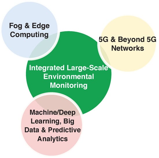
Figure 10.
Research areas playing a key role in future integrated large-scale environmental monitoring systems.
- Machine/deep learning, big data, and predictive analytics: According to a recent report by Cisco, the sole environmental data sensed by WSNs and crowdsensing nodes in urban environments are expected to increase up to 5 ZB per year by 2021 [444]. Such heterogeneous data are characterized by a large variability and large volumes and exhibit significantly different accuracy owing to the different types of sensors. In this respect, more advanced big data analytics need to be devised to extract meaningful information from a plethora of non-uniform raw environmental data, leveraging the joint processing power of both fixed and mobile nodes [445] and treating the whole ecosystem made of air and ground sensors as a smart and interconnected large-scale community [446], enabling the so-called smart environmental monitoring [37]. Machine/deep learning techniques represent another fundamental tool to manage large volumes of heterogeneous data for which analytical models are not often available [447]. Besides being used to enhance the performance of specific tasks such as, for instance, classification in hyperspectral imaging, such techniques can be extended also to support the design of optimal sensing strategies, with the aim of striking a sustainable balance between sensing quality and cost involved in the sensing campaign [448]. With the increasing availability of large environmental datasets, deep learning algorithms able to infer representations of data at different levels of abstraction will be also necessary [449]. As a fundamental enabler for most monitoring tasks, predictive analytics are required to combine big data and machine learning/deep learning and predict future evolution and impacts of environmental phenomena using both data-driven and model-based approaches [450].
- Fog computing and mobile edge computing: The potentially very high number of devices available when joining air and ground sensing capabilities over large geographical areas can seriously challenge most of the existing computing paradigms (e.g., cloud). A paradigm shift moving the intelligence closer to the sensing devices can represent a win–win strategy to guarantee a seamless environmental monitoring service while also fulfilling important requirements such as low-latency, availability of high dedicated bandwidths for data transfer, and context awareness for allocating sensing tasks and full support of node mobility [451]. Fog computing can suit such needs by making some of its multiple architectural layers available in the proximity of the sensing devices. Each layer is conceived with a significant processing, communication, and storage capability and is meant to support sensing nodes in performing preliminary local tasks [452]. Elaborating on the same idea, mobile edge computing aims at injecting application-oriented capabilities directly in the core of network operators, possibly providing most of the network and processing services at a one-hop distance from the sensing devices [453]. By working on top of secured peer-to-peer networks, sensing nodes can safely share the collected environmental data, whereas monitoring centers can have full control of the flow of sensed data [454].
- 5G and beyond 5G networks: The network infrastructure must be able to support different communication requirements according to the specific monitoring tasks and the involved sensing devices. For instance, UAV nodes require high availability of wireless links in order to be remotely piloted/controlled. Moreover, the periodic offloading of data from UAVs could involve several tens of GB, especially in the presence of data acquired by optical or hyperspectral sensors. On the other hand, crowdsensing nodes typically operate in urban environments, where signal obstruction phenomena (e.g., attenuation effects, multipath) are frequent owing to the presence of obstacles such as buildings, tunnels, and vehicles [455,456]. Supporting high data rates, ultra-reliable low-latency communications, and massive connectivity are among the main objectives of the emerging 5G cellular networks [457]. By exploiting the presence of multiple directional antennas at both the transmit and receive sides under the multiple-input multiple-output (MIMO) paradigm, 5G systems will guarantee more efficient wireless communications thanks to the beamforming technology, while simultaneously supporting critical services such as localization and context awareness [458,459]. In addition, communicating at mmWave frequencies allows for benefiting from higher bandwidths and, in turn, from higher data rates. Further improvements can be obtained by considering the use of the emerging reconfigurable intelligent surfaces (RIS). Such a technology, which will be at the basis of future 6G networks, allows wireless communications to evolve toward a new reality where the propagation environment can be re-engineered, i.e., dynamically programmed and reconfigured to adapt to the surrounding environment [460]. These artificial surfaces, made of electromagnetic material, can modify the propagation of radio waves (by acting the way that they interact with surrounding objects—see Figure 8, scenario A), thus attenuating the negative effects of propagation (path loss, multipath fading) and allowing for the establishment of a robust communication link even when the direct path between transmitter and receiver is severely obstructed. Notably, RISs are conceived as fully passive devices and as such represent a big promising step toward achieving pervasive but sustainable, reliable, and eco-friendly green communications [461,462].
7. Conclusions
The unprecedented environmental challenges faced by modern society call for the need of advanced solutions able to guarantee a pervasive and continuous monitoring of the environment in all its aspects (air, land, and water). With the increasing availability of WSN, UAV, and crowdsensing technologies, nowadays endorsed with significant sensing and processing capabilities, a new frontier of environmental monitoring empowered by a large number of low-cost devices and offering a denser and more accurate coverage of the territory has emerged. In this paper, we provided a systematic review of the main solutions proposed in the field of WSN, UAV, and crowdsensing monitoring, harmonizing the huge amount of work scattered across different research communities according to each specific application context (air, land, or sea). Based on such a classification, we highlighted the main benefits and open challenges of each individual technology. As a second main contribution, we analyzed the signal processing literature and conducted a detailed review of the most relevant methodologies applied in the field of environmental monitoring. Remarkably, it has been found that advanced signal processing plays a key role in a number of environmental tasks, from the choice of the optimal sites for sensor placement to the accurate reconstruction of physical phenomena and effective identification of polluted areas and natural hazards. We then identified the main components of a three-layer architecture that, by joining the ground and aerial sensing capabilities of WSN/crowdsensing and UAVs, can enable integrated and large-scale monitoring of the environment, leveraging advanced signal processing to promote cost-effectiveness and scalability. Finally, a perspective of future research directions has been provided, outlining that a synergy between different research areas is necessary to handle the intrinsic multi-disciplinarity of the topic.
Funding
This research received no external funding.
Institutional Review Board Statement
Not applicable.
Informed Consent Statement
Not applicable.
Data Availability Statement
The study did not report any data.
Acknowledgments
The author would like to thank Angelo Coluccia for the insightful discussions on the topic and the extensive review of the paper.
Conflicts of Interest
The author declares no conflict of interest.
References
- Climate Change 2021: The Physical Science Basis. In Contribution of Working Group I to the Sixth Assessment Report of the Intergovernmental Panel on Climate Change; Technical Report; Cambridge University Press: Cambridge, UK, 2021.
- WHO. 7 Million Premature Deaths Annually Linked to Air Pollution. Air Qual. Clim. Chang. 2014, 22, 53–59. [Google Scholar]
- Di, Q.; Wang, Y.; Zanobetti, A.; Wang, Y.; Koutrakis, P.; Choirat, C.; Dominici, F.; Schwartz, J.D. Air pollution and mortality in the Medicare population. N. Engl. J. Med. 2017, 376, 2513–2522. [Google Scholar] [CrossRef]
- Shuman, C.A.; Steffen, K.; Box, J.E.; Stearns, C.R. A dozen years of temperature observations at the Summit: Central Greenland automatic weather stations 1987–99. J. Appl. Meteorol. 2001, 40, 741–752. [Google Scholar] [CrossRef]
- Ringler, A.T.; Steim, J.; Wilson, D.C.; Widmer-Schnidrig, R.; Anthony, R.E. Improvements in seismic resolution and current limitations in the Global Seismographic Network. Geophys. J. Int. 2020, 220, 508–521. [Google Scholar] [CrossRef]
- Gasparin, F.; Greiner, E.; Lellouche, J.M.; Legalloudec, O.; Garric, G.; Drillet, Y.; Bourdallé-Badie, R.; Le Traon, P.Y.; Rémy, E.; Drévillon, M. A large-scale view of oceanic variability from 2007 to 2015 in the global high resolution monitoring and forecasting system at Mercator Océan. J. Mar. Syst. 2018, 187, 260–276. [Google Scholar] [CrossRef]
- Coluccia, A.; Fascista, A.; Ricci, G. CFAR Feature Plane: A Novel Framework for the Analysis and Design of Radar Detectors. IEEE Trans. Signal Process. 2020, 68, 3903–3916. [Google Scholar] [CrossRef]
- Coluccia, A.; Fascista, A.; Ricci, G. A k-nearest neighbors approach to the design of radar detectors. Signal Process. 2020, 174, 107609. [Google Scholar] [CrossRef]
- Coluccia, A.; Fascista, A.; Ricci, G. A novel approach to robust radar detection of range-spread targets. Signal Process. 2020, 166, 107223. [Google Scholar] [CrossRef]
- Coluccia, A.; Fascista, A.; Ricci, G. A KNN-Based Radar Detector for Coherent Targets in Non-Gaussian Noise. IEEE Signal Process. Lett. 2021, 28, 778–782. [Google Scholar] [CrossRef]
- Toth, C.; Jóźków, G. Remote sensing platforms and sensors: A survey. ISPRS J. Photogramm. Remote Sens. 2016, 115, 22–36. [Google Scholar] [CrossRef]
- Quang, T.N.; He, C.; Morawska, L.; Knibbs, L.D.; Falk, M. Vertical particle concentration profiles around urban office buildings. Atmos. Chem. Phys. 2012, 12, 5017–5030. [Google Scholar] [CrossRef]
- Li, T.; Shen, H.; Zeng, C.; Yuan, Q. A Validation Approach Considering the Uneven Distribution of Ground Stations for Satellite-Based PM2.5 Estimation. IEEE J. Sel. Top. Appl. Earth Obs. Remote Sens. 2020, 13, 1312–1321. [Google Scholar] [CrossRef]
- Lazarescu, M.T. Design of a WSN Platform for Long-Term Environmental Monitoring for IoT Applications. IEEE J. Emerg. Sel. Top. Circuits Syst. 2013, 3, 45–54. [Google Scholar] [CrossRef]
- Raza, M.; Aslam, N.; Le-Minh, H.; Hussain, S.; Cao, Y.; Khan, N.M. A critical analysis of research potential, challenges, and future directives in industrial wireless sensor networks. IEEE Commun. Surv. Tutor. 2017, 20, 39–95. [Google Scholar] [CrossRef]
- Grace, R.K.; Manju, S. A comprehensive review of wireless sensor networks based air pollution monitoring systems. Wirel. Pers. Commun. 2019, 108, 2499–2515. [Google Scholar] [CrossRef]
- Brito, T.; Pereira, A.I.; Lima, J.; Valente, A. Wireless Sensor Network for Ignitions Detection: An IoT approach. Electronics 2020, 9, 893. [Google Scholar] [CrossRef]
- Xu, G.; Shi, Y.; Sun, X.; Shen, W. Internet of Things in Marine Environment Monitoring: A Review. Sensors 2019, 19, 1711. [Google Scholar] [CrossRef]
- Messina, G.; Modica, G. Applications of UAV Thermal Imagery in Precision Agriculture: State of the Art and Future Research Outlook. Remote Sens. 2020, 12, 1491. [Google Scholar] [CrossRef]
- Boccardo, P.; Chiabrando, F.; Dutto, F.; Tonolo, F.G.; Lingua, A. UAV Deployment Exercise for Mapping Purposes: Evaluation of Emergency Response Applications. Sensors 2015, 15, 15717–15737. [Google Scholar] [CrossRef]
- Ejaz, W.; Azam, M.A.; Saadat, S.; Iqbal, F.; Hanan, A. Unmanned Aerial Vehicles enabled IoT Platform for Disaster Management. Energies 2019, 12, 2706. [Google Scholar] [CrossRef]
- Sestras, P.; Bilasco, S.; Rosca, S.; Dudic, B.; Hysa, A.; Spalevic, V. Geodetic and UAV Monitoring in the Sustainable Management of Shallow Landslides and Erosion of a Susceptible Urban Environment. Remote Sens. 2021, 13, 385. [Google Scholar] [CrossRef]
- Coluccia, A.; Fascista, A.; Schumann, A.; Sommer, L.; Dimou, A.; Zarpalas, D.; Méndez, M.; de la Iglesia, D.; González, I.; Mercier, J.P.; et al. Drone vs. Bird Detection: Deep Learning Algorithms and Results from a Grand Challenge. Sensors 2021, 21, 2824. [Google Scholar] [CrossRef] [PubMed]
- Coluccia, A.; Parisi, G.; Fascista, A. Detection and Classification of Multirotor Drones in Radar Sensor Networks: A Review. Sensors 2020, 20, 4172. [Google Scholar] [CrossRef]
- Coluccia, A.; Fascista, A.; Schumann, A.; Sommer, L.; Dimou, A.; Zarpalas, D.; Akyon, F.C.; Eryuksel, O.; Ozfuttu, K.A.; Altinuc, S.O.; et al. Drone-vs-Bird Detection Challenge at IEEE AVSS2021. In Proceedings of the 2021 17th IEEE International Conference on Advanced Video and Signal Based Surveillance (AVSS), Washington, DC, USA, 16–19 November 2021; pp. 1–8. [Google Scholar] [CrossRef]
- Habib, A.; Zhou, T.; Masjedi, A.; Zhang, Z.; Evan Flatt, J.; Crawford, M. Boresight Calibration of GNSS/INS-Assisted Push-Broom Hyperspectral Scanners on UAV Platforms. IEEE J. Sel. Top. Appl. Earth Obs. Remote Sens. 2018, 11, 1734–1749. [Google Scholar] [CrossRef]
- Coluccia, A.; Fascista, A.; Ricci, G. Online Estimation and Smoothing of a Target Trajectory in Mixed Stationary/moving Conditions. In Proceedings of the ICASSP 2019—2019 IEEE International Conference on Acoustics, Speech and Signal Processing (ICASSP), Brighton, UK, 12–17 May 2019; pp. 4445–4449. [Google Scholar] [CrossRef]
- Coluccia, A. Crowdsensing networks in the IoT age. Trans. Emerg. Telecommun. Technol. 2019, 30, e3621. [Google Scholar] [CrossRef]
- Chessa, S.; Corradi, A.; Foschini, L.; Girolami, M. Empowering mobile crowdsensing through social and ad hoc networking. IEEE Commun. Mag. 2016, 54, 108–114. [Google Scholar] [CrossRef]
- Aguiari, D.; Delnevo, G.; Monti, L.; Ghini, V.; Mirri, S.; Salomoni, P.; Pau, G.; Im, M.; Tse, R.; Ekpanyapong, M.; et al. Canarin II: Designing a smart e-bike eco-system. In Proceedings of the 2018 15th IEEE Annual Consumer Communications & Networking Conference (CCNC), Las Vegas, NV, USA, 12–15 January 2018; pp. 1–6. [Google Scholar]
- Calabrese, F.; Colonna, M.; Lovisolo, P.; Parata, D.; Ratti, C. Real-Time Urban Monitoring Using Cell Phones: A Case Study in Rome. IEEE Trans. Intell. Transp. Syst. 2011, 12, 141–151. [Google Scholar] [CrossRef]
- Chaturvedi, M.; Srivastava, S. Multi-Modal Design of an Intelligent Transportation System. IEEE Trans. Intell. Transp. Syst. 2017, 18, 2017–2027. [Google Scholar] [CrossRef]
- Wang, Z.; Pang, X.; Hu, J.; Liu, W.; Wang, Q.; Li, Y.; Chen, H. When Mobile Crowdsensing Meets Privacy. IEEE Commun. Mag. 2019, 57, 72–78. [Google Scholar] [CrossRef]
- Hart, J.K.; Martinez, K. Environmental Sensor Networks: A revolution in the earth system science? Earth-Sci. Rev. 2006, 78, 177–191. [Google Scholar] [CrossRef]
- Xu, G.; Shen, W.; Wang, X. Marine environment monitoring using Wireless Sensor Networks: A systematic review. In Proceedings of the 2014 IEEE International Conference on Systems, Man, and Cybernetics (SMC), San Diego, CA, USA, 5–8 October 2014; pp. 13–18. [Google Scholar] [CrossRef]
- Olatinwo, S.O.; Joubert, T.H. Energy Efficient Solutions in Wireless Sensor Systems for Water Quality Monitoring: A Review. IEEE Sens. J. 2019, 19, 1596–1625. [Google Scholar] [CrossRef]
- Ullo, S.L.; Sinha, G.R. Advances in Smart Environment Monitoring Systems Using IoT and Sensors. Sensors 2020, 20, 3113. [Google Scholar] [CrossRef]
- Francesc Alías, R.M.A.P. Review of Wireless Acoustic Sensor Networks for Environmental Noise Monitoring in Smart Cities. J. Sens. 2019, 2019, 7634860. [Google Scholar] [CrossRef]
- Jawad, H.M.; Nordin, R.; Gharghan, S.K.; Jawad, A.M.; Ismail, M. Energy-Efficient Wireless Sensor Networks for Precision Agriculture: A Review. Sensors 2017, 17, 1781. [Google Scholar] [CrossRef]
- Manfreda, S.; McCabe, M.F.; Miller, P.E.; Lucas, R.; Pajuelo Madrigal, V.; Mallinis, G.; Ben Dor, E.; Helman, D.; Estes, L.; Ciraolo, G.; et al. On the Use of Unmanned Aerial Systems for Environmental Monitoring. Remote Sens. 2018, 10, 641. [Google Scholar] [CrossRef]
- Tmušić, G.; Manfreda, S.; Aasen, H.; James, M.R.; Gonçalves, G.; Ben-Dor, E.; Brook, A.; Polinova, M.; Arranz, J.J.; Mészáros, J.; et al. Current Practices in UAS-based Environmental Monitoring. Remote Sens. 2020, 12, 1001. [Google Scholar] [CrossRef]
- Adão, T.; Hruška, J.; Pádua, L.; Bessa, J.; Peres, E.; Morais, R.; Sousa, J.J. Hyperspectral Imaging: A Review on UAV-Based Sensors, Data Processing and Applications for Agriculture and Forestry. Remote Sens. 2017, 9, 1110. [Google Scholar] [CrossRef]
- Ventura, D.; Bonifazi, A.; Gravina, M.F.; Ardizzone, G.D. Unmanned aerial systems (UASs) for environmental monitoring: A review with applications in coastal habitats. Aer. Robot.-Aerodyn. Control Appl. 2017, 165–184. [Google Scholar] [CrossRef]
- Barmpoutis, P.; Papaioannou, P.; Dimitropoulos, K.; Grammalidis, N. A Review on Early Forest Fire Detection Systems Using Optical Remote Sensing. Sensors 2020, 20, 6442. [Google Scholar] [CrossRef] [PubMed]
- Melis, M.T.; Da Pelo, S.; Erbì, I.; Loche, M.; Deiana, G.; Demurtas, V.; Meloni, M.A.; Dessì, F.; Funedda, A.; Scaioni, M.; et al. Thermal Remote Sensing from UAVs: A Review on Methods in Coastal Cliffs Prone to Landslides. Remote Sens. 2020, 12, 1971. [Google Scholar] [CrossRef]
- Lambey, V.; Prasad, A. A review on air quality measurement using an unmanned aerial vehicle. Water Air Soil Pollut. 2021, 232, 1–32. [Google Scholar] [CrossRef]
- Capponi, A.; Fiandrino, C.; Kantarci, B.; Foschini, L.; Kliazovich, D.; Bouvry, P. A Survey on Mobile Crowdsensing Systems: Challenges, Solutions, and Opportunities. IEEE Commun. Surv. Tutor. 2019, 21, 2419–2465. [Google Scholar] [CrossRef]
- Mamun, M.A.A.; Yuce, M.R. Sensors and Systems for Wearable Environmental Monitoring Toward IoT-Enabled Applications: A Review. IEEE Sens. J. 2019, 19, 7771–7788. [Google Scholar] [CrossRef]
- Sun, Y.; Ding, W.; Shu, L.; Li, K.; Zhang, Y.; Zhou, Z.; Han, G. On Enabling Mobile Crowd Sensing for Data Collection in Smart Agriculture: A Vision. IEEE Syst. J. 2021, 1–12. [Google Scholar] [CrossRef]
- Abualsaud, K.; Elfouly, T.M.; Khattab, T.; Yaacoub, E.; Ismail, L.S.; Ahmed, M.H.; Guizani, M. A Survey on Mobile Crowd-Sensing and Its Applications in the IoT Era. IEEE Access 2019, 7, 3855–3881. [Google Scholar] [CrossRef]
- Phengsuwan, J.; Shah, T.; Thekkummal, N.B.; Wen, Z.; Sun, R.; Pullarkatt, D.; Thirugnanam, H.; Ramesh, M.V.; Morgan, G.; James, P.; et al. Use of Social Media Data in Disaster Management: A Survey. Future Internet 2021, 13, 46. [Google Scholar] [CrossRef]
- Popescu, D.; Stoican, F.; Stamatescu, G.; Chenaru, O.; Ichim, L. A Survey of Collaborative UAV–WSN Systems for Efficient Monitoring. Sensors 2019, 19, 4690. [Google Scholar] [CrossRef]
- Erdelj, M.; Król, M.; Natalizio, E. Wireless sensor networks and multi-UAV systems for natural disaster management. Comput. Netw. 2017, 124, 72–86. [Google Scholar] [CrossRef]
- Carminati, M.; Kanoun, O.; Ullo, S.L.; Marcuccio, S. Prospects of Distributed Wireless Sensor Networks for Urban Environmental Monitoring. IEEE Aerosp. Electron. Syst. Mag. 2019, 34, 44–52. [Google Scholar] [CrossRef]
- Justino, C.I.L.; Duarte, A.C.; Rocha-Santos, T.A.P. Recent Progress in Biosensors for Environmental Monitoring: A Review. Sensors 2017, 17, 2918. [Google Scholar] [CrossRef]
- Moore, T.S.; Mullaugh, K.M.; Holyoke, R.R.; Madison, A.S.; Yücel, M.; Luther, G.W. Marine Chemical Technology and Sensors for Marine Waters: Potentials and Limits. Annu. Rev. Mar. Sci. 2009, 1, 91–115. [Google Scholar] [CrossRef]
- Kassal, P.; Steinberg, M.D.; Steinberg, I.M. Wireless chemical sensors and biosensors: A review. Sens. Actuators B Chem. 2018, 266, 228–245. [Google Scholar] [CrossRef]
- Majhi, S.M.; Mirzaei, A.; Kim, H.W.; Kim, S.S.; Kim, T.W. Recent advances in energy-saving chemiresistive gas sensors: A review. Nano Energy 2021, 79, 105369. [Google Scholar] [CrossRef]
- Hernandez-Vargas, G.; Sosa-Hernández, J.E.; Saldarriaga-Hernandez, S.; Villalba-Rodríguez, A.M.; Parra-Saldivar, R.; Iqbal, H.M.N. Electrochemical Biosensors: A Solution to Pollution Detection with Reference to Environmental Contaminants. Biosensors 2018, 8, 29. [Google Scholar] [CrossRef]
- Allen, M.F.; Vargas, R.; Graham, E.A.; Swenson, W.; Hamilton, M.; Taggart, M.; Harmon, T.C.; Rat’Ko, A.; Rundel, P.; Fulkerson, B.; et al. Soil Sensor Technology: Life within a Pixel. BioScience 2007, 57, 859–867. [Google Scholar] [CrossRef]
- Dobre, A.; Arnold, S.; Smalley, R.; Boddy, J.; Barlow, J.; Tomlin, A.; Belcher, S. Flow field measurements in the proximity of an urban intersection in London, UK. Atmos. Environ. 2005, 39, 4647–4657. [Google Scholar] [CrossRef]
- Murty, R.N.; Mainland, G.; Rose, I.; Chowdhury, A.R.; Gosain, A.; Bers, J.; Welsh, M. CitySense: An Urban-Scale Wireless Sensor Network and Testbed. In Proceedings of the 2008 IEEE Conference on Technologies for Homeland Security, Waltham, MA, USA, 12–13 May 2008; pp. 583–588. [Google Scholar] [CrossRef]
- Kadri, A.; Yaacoub, E.; Mushtaha, M.; Abu-Dayya, A. Wireless sensor network for real-time air pollution monitoring. In Proceedings of the 2013 1st International Conference on Communications, Signal Processing, and their Applications (ICCSPA), Sharjah, United Arab Emirates, 12–14 February 2013; pp. 1–5. [Google Scholar] [CrossRef]
- Mansour, S.; Nasser, N.; Karim, L.; Ali, A. Wireless Sensor Network-based air quality monitoring system. In Proceedings of the 2014 International Conference on Computing, Networking and Communications (ICNC), Honolulu, HI, USA, 3–6 February 2014; pp. 545–550. [Google Scholar] [CrossRef]
- Kularatna, N.; Sudantha, B.H. An Environmental Air Pollution Monitoring System Based on the IEEE 1451 Standard for Low Cost Requirements. IEEE Sens. J. 2008, 8, 415–422. [Google Scholar] [CrossRef]
- Postolache, O.A.; Dias Pereira, J.M.; Silva Girao, P.M.B. Smart Sensors Network for Air Quality Monitoring Applications. IEEE Trans. Instrum. Meas. 2009, 58, 3253–3262. [Google Scholar] [CrossRef]
- Lay-Ekuakille, A.; Trotta, A. Predicting VOC Concentration Measurements: Cognitive Approach for Sensor Networks. IEEE Sens. J. 2011, 11, 3023–3030. [Google Scholar] [CrossRef]
- Yan, R.; Sun, H.; Qian, Y. Energy-Aware Sensor Node Design With Its Application in Wireless Sensor Networks. IEEE Trans. Instrum. Meas. 2013, 62, 1183–1191. [Google Scholar] [CrossRef]
- Jelicic, V.; Magno, M.; Brunelli, D.; Paci, G.; Benini, L. Context-Adaptive Multimodal Wireless Sensor Network for Energy-Efficient Gas Monitoring. IEEE Sens. J. 2013, 13, 328–338. [Google Scholar] [CrossRef]
- Gedik, B.; Liu, L. A scalable peer-to-peer architecture for distributed information monitoring applications. IEEE Trans. Comput. 2005, 54, 767–782. [Google Scholar] [CrossRef]
- Lombardo, L.; Corbellini, S.; Parvis, M.; Elsayed, A.; Angelini, E.; Grassini, S. Wireless Sensor Network for Distributed Environmental Monitoring. IEEE Trans. Instrum. Meas. 2018, 67, 1214–1222. [Google Scholar] [CrossRef]
- Fuertes, W.; Carrera, D.; Villacís, C.; Toulkeridis, T.; Galárraga, F.; Torres, E.; Aules, H. Distributed System as Internet of Things for a New Low-Cost, Air Pollution Wireless Monitoring on Real Time. In Proceedings of the 2015 IEEE/ACM 19th International Symposium on Distributed Simulation and Real Time Applications (DS-RT), Chengdu, China, 14–16 October 2015; pp. 58–67. [Google Scholar] [CrossRef]
- Corbellini, S.; Parvis, M. Wireless sensor network architecture for remote non-invasive museum monitoring. In Proceedings of the 2016 IEEE International Symposium on Systems Engineering (ISSE), Edinburgh, UK, 3–5 October 2016; pp. 1–7. [Google Scholar] [CrossRef]
- Boubrima, A.; Bechkit, W.; Rivano, H. Optimal WSN Deployment Models for Air Pollution Monitoring. IEEE Trans. Wirel. Commun. 2017, 16, 2723–2735. [Google Scholar] [CrossRef]
- Boubrima, A.; Bechkit, W.; Rivano, H. On the Deployment of Wireless Sensor Networks for Air Quality Mapping: Optimization Models and Algorithms. IEEE/ACM Trans. Netw. 2019, 27, 1629–1642. [Google Scholar] [CrossRef]
- Boubrima, A.; Bechkit, W.; Rivano, H. Error-Bounded Air Quality Mapping Using Wireless Sensor Networks. In Proceedings of the 2016 IEEE 41st Conference on Local Computer Networks (LCN), Dubai, United Arab Emirates, 7–10 November 2016; pp. 380–388. [Google Scholar] [CrossRef]
- Luo, L.; Qin, H.; Song, X.; Wang, M.; Qiu, H.; Zhou, Z. Wireless Sensor Networks for Noise Measurement and Acoustic Event Recognitions in Urban Environments. Sensors 2020, 20, 2093. [Google Scholar] [CrossRef] [PubMed]
- Allegro, G.; Fascista, A.; Coluccia, A. Acoustic Dual-Function Communication and Echo-Location in Inaudible Band. Sensors 2022, 22, 1284. [Google Scholar] [CrossRef]
- Bertrand, A.; Doclo, S.; Gannot, S.; Ono, N.; van Waterschoot, T. Special issue on wireless acoustic sensor networks and ad hoc microphone arrays. Signal Process. 2015, 107, 1–3. [Google Scholar] [CrossRef]
- Markovich-Golan, S.; Bertrand, A.; Moonen, M.; Gannot, S. Optimal distributed minimum-variance beamforming approaches for speech enhancement in wireless acoustic sensor networks. Signal Process. 2015, 107, 4–20. [Google Scholar] [CrossRef]
- Griffin, A.; Alexandridis, A.; Pavlidi, D.; Mastorakis, Y.; Mouchtaris, A. Localizing multiple audio sources in a wireless acoustic sensor network. Signal Process. 2015, 107, 54–67. [Google Scholar] [CrossRef]
- Taghizadeh, M.J.; Parhizkar, R.; Garner, P.N.; Bourlard, H.; Asaei, A. Ad hoc microphone array calibration: Euclidean distance matrix completion algorithm and theoretical guarantees. Signal Process. 2015, 107, 123–140. [Google Scholar] [CrossRef]
- Hassani, A.; Bertrand, A.; Moonen, M. Cooperative integrated noise reduction and node-specific direction-of-arrival estimation in a fully connected wireless acoustic sensor network. Signal Process. 2015, 107, 68–81. [Google Scholar] [CrossRef]
- Botteldooren, D.; De Coensel, B.; Oldoni, D.; Van Renterghem, T.; Dauwe, S. Sound monitoring networks new style. In Acoustics 2011: Breaking New Ground: Proceedings of the Annual Conference of the Australian Acoustical Society; Mee, J., David, H., Ian, D.M., Eds.; Australian Acoustical Society: Gold Coast, Australia, 2011; pp. 93:1–93:5. [Google Scholar]
- Farrés, J.C.; Novas, J.C. Issues and challenges to improve the Barcelona Noise Monitoring Network. In Proceedings of the 11th European Congress and Exposition on Noise Control Engineering, Heraklion, Crete, Greece, 27–31 May 2018; pp. 27–31. [Google Scholar]
- Nave, L.; Mietlicki, F. Medusa, a new approach for noise management and control in urban environment. In Proceedings of the INTER-NOISE and NOISE-CON Congress and Conference Proceedings, Virginia, VA, USA, 16–19 June 2019; Institute of Noise Control Engineering: Virginia, VA, USA, 2019; Volume 259, pp. 2411–2419. [Google Scholar]
- Rainham, D. A wireless sensor network for urban environmental health monitoring: UrbanSense. IOP Conf. Ser. Earth Environ. Sci. 2016, 34, 012028. [Google Scholar] [CrossRef]
- Bartalucci, C.; Borchi, F.; Carfagni, M.; Furferi, R.; Governi, L.; Lapini, A.; Bellomini, R.; Luzzi, S.; Nencini, L. The smart noise monitoring system implemented in the frame of the Life MONZA project. In Proceedings of the EuroNoise, Crete, Greece, 27–31 May 2018; pp. 783–788. [Google Scholar]
- Vinci, B.; Tonacci, A.; Caudai, C.; De Rosa, P.; Nencini, L.; Pratali, L. The SENSEable Pisa Project: Citizen-Participation in Monitoring Acoustic Climate of Mediterranean City Centers. CLEAN–Soil Air Water 2017, 45, 1600137. [Google Scholar] [CrossRef]
- Hoornweg, D.; Bhada-Tata, P.; Kennedy, C. Environment: Waste production must peak this century. Nat. News 2013, 502, 615. [Google Scholar] [CrossRef]
- Sunny, A.I.; Zhao, A.; Li, L.; Kanteh Sakiliba, S. Low-Cost IoT-Based Sensor System: A Case Study on Harsh Environmental Monitoring. Sensors 2021, 21, 214. [Google Scholar] [CrossRef]
- Gomaa, R.I.; Shohdy, I.A.; Sharshar, K.A.; Al-Kabbani, A.S.; Ragai, H.F. Real-Time Radiological Monitoring of Nuclear Facilities Using ZigBee Technology. IEEE Sens. J. 2014, 14, 4007–4013. [Google Scholar] [CrossRef]
- Zhang, K.; Li, Y.; XIiao, W.H.; Suh, H. The Application of a Wireless Sensor Network Design Based on ZigBee in Petrochemical Industry Field. In Proceedings of the 2008 First International Conference on Intelligent Networks and Intelligent Systems, Wuhan, China, 1–3 November 2008; pp. 284–287. [Google Scholar] [CrossRef]
- El Kouche, A.; Al-Awami, L.; Hassanein, H.; Obaia, K. WSN application in the harsh industrial environment of the oil sands. In Proceedings of the 2011 7th International Wireless Communications and Mobile Computing Conference, Istanbul, Turkey, 4–8 July 2011; pp. 613–618. [Google Scholar] [CrossRef]
- Hodge, V.J.; O’Keefe, S.; Weeks, M.; Moulds, A. Wireless Sensor Networks for Condition Monitoring in the Railway Industry: A Survey. IEEE Trans. Intell. Transp. Syst. 2015, 16, 1088–1106. [Google Scholar] [CrossRef]
- Tang, C.; Rashvand, H.F.; Tian, G.Y.; Hu, P.; Sunny, A.I.; Wang, H. Structural health monitoring with WSNs. Wirel. Sens. Syst. Extrem. Environ. Space Underw. Undergr. Ind. 2017, 383–408. [Google Scholar]
- Williams, A.J.; Torquato, M.F.; Cameron, I.M.; Fahmy, A.A.; Sienz, J. Survey of Energy Harvesting Technologies for Wireless Sensor Networks. IEEE Access 2021, 9, 77493–77510. [Google Scholar] [CrossRef]
- Prauzek, M.; Konecny, J.; Borova, M.; Janosova, K.; Hlavica, J.; Musilek, P. Energy Harvesting Sources, Storage Devices and System Topologies for Environmental Wireless Sensor Networks: A Review. Sensors 2018, 18, 2446. [Google Scholar] [CrossRef]
- Vega-Rodríguez, R.; Sendra, S.; Lloret, J.; Romero-Díaz, P.; Garcia-Navas, J.L. Low Cost LoRa based Network for Forest Fire Detection. In Proceedings of the 2019 Sixth International Conference on Internet of Things: Systems, Management and Security (IOTSMS), Granada, Spain, 22–25 October 2019; pp. 177–184. [Google Scholar] [CrossRef]
- Ramelan, A.; Hamka Ibrahim, M.; Chico Hermanu Brillianto, A.; Adriyanto, F.; Rizqi Subeno, M.; Latifah, A. A Preliminary Prototype of LoRa-Based Wireless Sensor Network for Forest Fire Monitoring. In Proceedings of the 2021 International Conference on ICT for Smart Society (ICISS), Bandung, Indonesia, 2–4 August 2021; pp. 1–5. [Google Scholar] [CrossRef]
- Verma, S.; Kaur, S.; Rawat, D.B.; Xi, C.; Alex, L.T.; Zaman Jhanjhi, N. Intelligent Framework Using IoT-Based WSNs for Wildfire Detection. IEEE Access 2021, 9, 48185–48196. [Google Scholar] [CrossRef]
- Giorgetti, A.; Lucchi, M.; Tavelli, E.; Barla, M.; Gigli, G.; Casagli, N.; Chiani, M.; Dardari, D. A Robust Wireless Sensor Network for Landslide Risk Analysis: System Design, Deployment, and Field Testing. IEEE Sens. J. 2016, 16, 6374–6386. [Google Scholar] [CrossRef]
- Jeong, S.; Ko, J.; Kim, J. The Effectiveness of a Wireless Sensor Network System for Landslide Monitoring. IEEE Access 2020, 8, 8073–8086. [Google Scholar] [CrossRef]
- Ramesh, M.V. Design, development, and deployment of a wireless sensor network for detection of landslides. Ad Hoc Netw. 2014, 13, 2–18. [Google Scholar] [CrossRef]
- Ojha, T.; Misra, S.; Raghuwanshi, N.S. Wireless sensor networks for agriculture: The state-of-the-art in practice and future challenges. Comput. Electron. Agric. 2015, 118, 66–84. [Google Scholar] [CrossRef]
- Srbinovska, M.; Gavrovski, C.; Dimcev, V.; Krkoleva, A.; Borozan, V. Environmental parameters monitoring in precision agriculture using wireless sensor networks. J. Clean. Prod. 2015, 88, 297–307. [Google Scholar] [CrossRef]
- Thakur, D.; Kumar, Y.; Kumar, A.; Singh, P.K. Applicability of wireless sensor networks in precision agriculture: A review. Wirel. Pers. Commun. 2019, 107, 471–512. [Google Scholar] [CrossRef]
- Kim, Y.; Evans, R.G.; Iversen, W.M. Remote Sensing and Control of an Irrigation System Using a Distributed Wireless Sensor Network. IEEE Trans. Instrum. Meas. 2008, 57, 1379–1387. [Google Scholar] [CrossRef]
- Gutiérrez, J.; Villa-Medina, J.F.; Nieto-Garibay, A.; Porta-Gándara, M.A. Automated Irrigation System Using a Wireless Sensor Network and GPRS Module. IEEE Trans. Instrum. Meas. 2014, 63, 166–176. [Google Scholar] [CrossRef]
- Burak, S.; Dogan, E.; Gazioglu, C. Impact of urbanization and tourism on coastal environment. Ocean. Coast. Manag. 2004, 47, 515–527. [Google Scholar] [CrossRef]
- Albaladejo Pérez, C.; Soto Valles, F.; Torres Sánchez, R.; Jiménez Buendía, M.; López-Castejón, F.; Gilabert Cervera, J. Design and Deployment of a Wireless Sensor Network for the Mar Menor Coastal Observation System. IEEE J. Ocean. Eng. 2017, 42, 966–976. [Google Scholar] [CrossRef]
- Adamo, F.; Attivissimo, F.; Carducci, C.G.C.; Lanzolla, A.M.L. A Smart Sensor Network for Sea Water Quality Monitoring. IEEE Sens. J. 2015, 15, 2514–2522. [Google Scholar] [CrossRef]
- Bloecher, N.; Solvang, T.; Floerl, O. Efficacy testing of novel antifouling systems for marine sensors. Ocean. Eng. 2021, 240, 109983. [Google Scholar] [CrossRef]
- Delgado, A.; Briciu-Burghina, C.; Regan, F. Antifouling Strategies for Sensors Used in Water Monitoring: Review and Future Perspectives. Sensors 2021, 21, 389. [Google Scholar] [CrossRef] [PubMed]
- Falleni, S.; Unal, D.; Neerman, A.; Enhos, K.; Demirors, E.; Basagni, S.; Melodia, T. Design, Development, and Testing of a Smart Buoy for Underwater Testbeds in Shallow Waters. In Proceedings of the Global Oceans 2020: Singapore–U.S. Gulf Coast, Biloxi, MS, USA, 5–30 October 2020; pp. 1–7. [Google Scholar] [CrossRef]
- Alippi, C.; Camplani, R.; Galperti, C.; Roveri, M. A Robust, Adaptive, Solar-Powered WSN Framework for Aquatic Environmental Monitoring. IEEE Sens. J. 2011, 11, 45–55. [Google Scholar] [CrossRef]
- Joshi, K.B.; Costello, J.H.; Priya, S. Estimation of Solar Energy Harvested for Autonomous Jellyfish Vehicles (AJVs). IEEE J. Ocean. Eng. 2011, 36, 539–551. [Google Scholar] [CrossRef]
- Jenkins, P.P.; Messenger, S.; Trautz, K.M.; Maximenko, S.I.; Goldstein, D.; Scheiman, D.; Hoheisel, R.; Walters, R.J. High-bandgap solar cells for underwater photovoltaic applications. IEEE J. Photovoltaics 2013, 4, 202–207. [Google Scholar] [CrossRef]
- Toma, D.M.; del Rio, J.; Carbonell-Ventura, M.; Masalles, J.M. Underwater energy harvesting system based on plucked-driven piezoelectrics. In Proceedings of the OCEANS 2015-Genova, Genova, Italy, 18–21 May 2015; pp. 1–5. [Google Scholar] [CrossRef]
- Wang, J.; Zhou, H.; Li, Y.; Sun, Q.; Wu, Y.; Jin, S.; Quek, T.Q.S.; Xu, C. Wireless Channel Models for Maritime Communications. IEEE Access 2018, 6, 68070–68088. [Google Scholar] [CrossRef]
- Shahanaghi, A.; Yang, Y.; Buehrer, R.M. Stochastic Link Modeling of Static Wireless Sensor Networks Over the Ocean Surface. IEEE Trans. Wirel. Commun. 2020, 19, 4154–4169. [Google Scholar] [CrossRef]
- Rani, S.; Ahmed, S.H.; Malhotra, J.; Talwar, R. Energy efficient chain based routing protocol for underwater wireless sensor networks. J. Netw. Comput. Appl. 2017, 92, 42–50. [Google Scholar] [CrossRef]
- Zhao, R.; Long, H.; Dobre, O.A.; Shen, X.; Ngatched, T.M.N.; Mei, H. Time Reversal Based MAC for Multi-Hop Underwater Acoustic Networks. IEEE Syst. J. 2019, 13, 2531–2542. [Google Scholar] [CrossRef]
- Devi, L.N.; Reddy, G.K.; Rao, A.N. Live Demonstration on Smart Water Quality Monitoring System Using Wireless Sensor Networks. In Proceedings of the 2018 IEEE SENSORS, New Delhi, India, 28–31 October 2018; pp. 1–4. [Google Scholar] [CrossRef]
- Wang, Y.; Rajib, S.M.S.M.; Collins, C.; Grieve, B. Low-Cost Turbidity Sensor for Low-Power Wireless Monitoring of Fresh-Water Courses. IEEE Sens. J. 2018, 18, 4689–4696. [Google Scholar] [CrossRef]
- Rosero-Montalvo, P.D.; López-Batista, V.F.; Riascos, J.A.; Peluffo-Ordóñez, D.H. Intelligent WSN System for Water Quality Analysis Using Machine Learning Algorithms: A Case Study (Tahuando River from Ecuador). Remote Sens. 2020, 12, 1988. [Google Scholar] [CrossRef]
- Lambrou, T.P.; Anastasiou, C.C.; Panayiotou, C.G.; Polycarpou, M.M. A Low-Cost Sensor Network for Real-Time Monitoring and Contamination Detection in Drinking Water Distribution Systems. IEEE Sens. J. 2014, 14, 2765–2772. [Google Scholar] [CrossRef]
- Mao, Y.; Qi, H.; Chen, X.; Li, X. Event Detection with Multivariate Water Parameters in the Water Monitoring Applications. In Proceedings of the 2017 IEEE 4th International Conference on Cyber Security and Cloud Computing (CSCloud), New York, NY, USA, 26–28 June 2017; pp. 321–326. [Google Scholar] [CrossRef]
- Wu, T.; Yang, P.; Dai, H.; Xu, W.; Xu, M. Charging Oriented Sensor Placement and Flexible Scheduling in Rechargeable WSNs. In Proceedings of the IEEE INFOCOM 2019—IEEE Conference on Computer Communications, Paris, France, 29 April–2 May 2019; pp. 73–81. [Google Scholar] [CrossRef]
- Chowdhury, S.A.; Benslimane, A.; Akhter, F. Autonomous Mobile Chargers for Rechargeable Sensor Networks Using Space Filling Curve. In Proceedings of the 2018 IEEE International Conference on Communications (ICC), Kansas City, MO, USA, 20–24 May 2018; pp. 1–6. [Google Scholar] [CrossRef]
- Kan, Y.; Chang, C.Y.; Kuo, C.H.; Roy, D.S. Coverage and Connectivity Aware Energy Charging Mechanism Using Mobile Charger for WRSNs. IEEE Syst. J. 2021, 1–12. [Google Scholar] [CrossRef]
- Pino, T.; Choudhury, S.; Al-Turjman, F. Dominating Set Algorithms for Wireless Sensor Networks Survivability. IEEE Access 2018, 6, 17527–17532. [Google Scholar] [CrossRef]
- Song, L.; Liu, C.; Huang, H.; Du, H.; Jia, X. Minimum Connected Dominating Set Under Routing Cost Constraint in Wireless Sensor Networks With Different Transmission Ranges. IEEE/ACM Trans. Netw. 2019, 27, 546–559. [Google Scholar] [CrossRef]
- Li, K.; Gao, X.; Wu, F.; Chen, G. A Constant Factor Approximation for d-Hop Connected Dominating Set in Three-Dimensional Wireless Networks. IEEE Trans. Wirel. Commun. 2019, 18, 4357–4367. [Google Scholar] [CrossRef]
- Swain, A.R.; Hansdah, R. A model for the classification and survey of clock synchronization protocols in WSNs. Ad Hoc Netw. 2015, 27, 219–241. [Google Scholar] [CrossRef]
- Maggs, M.K.; O’Keefe, S.G.; Thiel, D.V. Consensus Clock Synchronization for Wireless Sensor Networks. IEEE Sens. J. 2012, 12, 2269–2277. [Google Scholar] [CrossRef]
- Upadhyay, D.; Dubey, A.K.; Thilagam, P.S. Application of Non-Linear Gaussian Regression-Based Adaptive Clock Synchronization Technique for Wireless Sensor Network in Agriculture. IEEE Sens. J. 2018, 18, 4328–4335. [Google Scholar] [CrossRef]
- Noh, K.L.; Chaudhari, Q.M.; Serpedin, E.; Suter, B.W. Novel Clock Phase Offset and Skew Estimation Using Two-Way Timing Message Exchanges for Wireless Sensor Networks. IEEE Trans. Commun. 2007, 55, 766–777. [Google Scholar] [CrossRef]
- Tian, Y.P. Time Synchronization in WSNs With Random Bounded Communication Delays. IEEE Trans. Autom. Control 2017, 62, 5445–5450. [Google Scholar] [CrossRef]
- Toro, F.G.; Tsourdos, A. UAV Sensors for Environmental Monitoring; MDPI: Basel, Switzerland, 2018. [Google Scholar]
- Cichowicz, R.; Dobrzański, M. Spatial Analysis (Measurements at Heights of 10 m and 20 m above Ground Level) of the Concentrations of Particulate Matter (PM10, PM2.5, and PM1.0) and Gaseous Pollutants (H2S) on the University Campus: A Case Study. Atmosphere 2021, 12, 62. [Google Scholar] [CrossRef]
- Bolla, G.M.; Casagrande, M.; Comazzetto, A.; Dal Moro, R.; Destro, M.; Fantin, E.; Colombatti, G.; Aboudan, A.; Lorenzini, E.C. ARIA: Air Pollutants Monitoring Using UAVs. In Proceedings of the 2018 5th IEEE International Workshop on Metrology for AeroSpace (MetroAeroSpace), Rome, Italy, 20–22 June 2018; pp. 225–229. [Google Scholar] [CrossRef]
- Villa, T.F.; Gonzalez, F.; Miljievic, B.; Ristovski, Z.D.; Morawska, L. An Overview of Small Unmanned Aerial Vehicles for Air Quality Measurements: Present Applications and Future Prospectives. Sensors 2016, 16, 1072. [Google Scholar] [CrossRef]
- Rossi, M.; Brunelli, D.; Adami, A.; Lorenzelli, L.; Menna, F.; Remondino, F. Gas-Drone: Portable gas sensing system on UAVs for gas leakage localization. In Proceedings of the SENSORS, 2014 IEEE, Valencia, Spain, 2–5 November 2014; pp. 1431–1434. [Google Scholar] [CrossRef]
- Alvarado, M.; Gonzalez, F.; Erskine, P.; Cliff, D.; Heuff, D. A Methodology to Monitor Airborne PM10 Dust Particles Using a Small Unmanned Aerial Vehicle. Sensors 2017, 17, 343. [Google Scholar] [CrossRef]
- Kuantama, E.; Tarca, R.; Dzitac, S.; Dzitac, I.; Vesselenyi, T.; Tarca, I. The Design and Experimental Development of Air Scanning Using a Sniffer Quadcopter. Sensors 2019, 19, 3849. [Google Scholar] [CrossRef]
- Roldán, J.J.; Joossen, G.; Sanz, D.; Del Cerro, J.; Barrientos, A. Mini-UAV Based Sensory System for Measuring Environmental Variables in Greenhouses. Sensors 2015, 15, 3334–3350. [Google Scholar] [CrossRef]
- Gu, Q.; R. Michanowicz, D.; Jia, C. Developing a Modular Unmanned Aerial Vehicle (UAV) Platform for Air Pollution Profiling. Sensors 2018, 18, 4363. [Google Scholar] [CrossRef]
- He, X.; Bourne, J.R.; Steiner, J.A.; Mortensen, C.; Hoffman, K.C.; Dudley, C.J.; Rogers, B.; Cropek, D.M.; Leang, K.K. Autonomous Chemical-Sensing Aerial Robot for Urban/Suburban Environmental Monitoring. IEEE Syst. J. 2019, 13, 3524–3535. [Google Scholar] [CrossRef]
- Gao, J.; Hu, Z.; Bian, K.; Mao, X.; Song, L. AQ360: UAV-Aided Air Quality Monitoring by 360-Degree Aerial Panoramic Images in Urban Areas. IEEE Internet Things J. 2021, 8, 428–442. [Google Scholar] [CrossRef]
- Yang, Y.; Zheng, Z.; Bian, K.; Song, L.; Han, Z. Real-Time Profiling of Fine-Grained Air Quality Index Distribution Using UAV Sensing. IEEE Internet Things J. 2018, 5, 186–198. [Google Scholar] [CrossRef]
- Feng, L.; Tian, H.; Qiao, Z.; Zhao, M.; Liu, Y. Detailed Variations in Urban Surface Temperatures Exploration Based on Unmanned Aerial Vehicle Thermography. IEEE J. Sel. Top. Appl. Earth Obs. Remote Sens. 2020, 13, 204–216. [Google Scholar] [CrossRef]
- Cui, J.; Liu, M.; Zhang, Z.; Yang, S.; Ning, J. Robust UAV Thermal Infrared Remote Sensing Images Stitching Via Overlap-Prior-Based Global Similarity Prior Model. IEEE J. Sel. Top. Appl. Earth Obs. Remote Sens. 2021, 14, 270–282. [Google Scholar] [CrossRef]
- Shen, F.; Ding, G.; Wang, Z.; Wu, Q. UAV-Based 3D Spectrum Sensing in Spectrum-Heterogeneous Networks. IEEE Trans. Veh. Technol. 2019, 68, 5711–5722. [Google Scholar] [CrossRef]
- Salvati, D.; Drioli, C.; Ferrin, G.; Foresti, G.L. Acoustic Source Localization From Multirotor UAVs. IEEE Trans. Ind. Electron. 2020, 67, 8618–8628. [Google Scholar] [CrossRef]
- Stuart, M.B.; McGonigle, A.J.S.; Willmott, J.R. Hyperspectral Imaging in Environmental Monitoring: A Review of Recent Developments and Technological Advances in Compact Field Deployable Systems. Sensors 2019, 19, 3071. [Google Scholar] [CrossRef]
- Vohland, M.; Jung, A. Hyperspectral Imaging for Fine to Medium Scale Applications in Environmental Sciences. Remote Sens. 2020, 12, 2962. [Google Scholar] [CrossRef]
- Yao, H.; Qin, R.; Chen, X. Unmanned Aerial Vehicle for Remote Sensing Applications—A Review. Remote Sens. 2019, 11, 1443. [Google Scholar] [CrossRef]
- Youme, O.; Bayet, T.; Dembele, J.M.; Cambier, C. Deep Learning and Remote Sensing: Detection of Dumping Waste Using UAV. Procedia Comput. Sci. 2021, 185, 361–369. [Google Scholar] [CrossRef]
- Filkin, T.; Sliusar, N.; Ritzkowski, M.; Huber-Humer, M. Unmanned Aerial Vehicles for Operational Monitoring of Landfills. Drones 2021, 5, 125. [Google Scholar] [CrossRef]
- Zhang, Y.; Xu, Y.; Xiong, W.; Qu, R.; Ten, J.; Lou, Q.; Lv, N. Inversion Study of Heavy Metals in Soils of Potentially Polluted Sites Based on UAV Hyperspectral Data and Machine Learning Algorithms. In Proceedings of the 2021 11th Workshop on Hyperspectral Imaging and Signal Processing: Evolution in Remote Sensing (WHISPERS), Amsterdam, The Netherlands, 24–26 March 2021; pp. 1–5. [Google Scholar] [CrossRef]
- He, Y.; Ma, W.; Ma, Z.; Fu, W.; Chen, C.; Yang, C.F.; Liu, Z. Using Unmanned Aerial Vehicle Remote Sensing and a Monitoring Information System to Enhance the Management of Unauthorized Structures. Appl. Sci. 2019, 9, 4954. [Google Scholar] [CrossRef]
- Tewkesbury, A.P.; Comber, A.J.; Tate, N.J.; Lamb, A.; Fisher, P.F. A critical synthesis of remotely sensed optical image change detection techniques. Remote Sens. Environ. 2015, 160, 1–14. [Google Scholar] [CrossRef]
- Sudhakar, S.; Vijayakumar, V.; Sathiya Kumar, C.; Priya, V.; Ravi, L.; Subramaniyaswamy, V. Unmanned Aerial Vehicle (UAV) based Forest Fire Detection and monitoring for reducing false alarms in forest-fires. Comput. Commun. 2020, 149, 1–16. [Google Scholar] [CrossRef]
- Akhloufi, M.A.; Couturier, A.; Castro, N.A. Unmanned Aerial Vehicles for Wildland Fires: Sensing, Perception, Cooperation and Assistance. Drones 2021, 5, 15. [Google Scholar] [CrossRef]
- Bouguettaya, A.; Zarzour, H.; Taberkit, A.M.; Kechida, A. A review on early wildfire detection from unmanned aerial vehicles using deep learning-based computer vision algorithms. Signal Process. 2022, 190, 108309. [Google Scholar] [CrossRef]
- Barmpoutis, P.; Stathaki, T.; Dimitropoulos, K.; Grammalidis, N. Early Fire Detection Based on Aerial 360-Degree Sensors, Deep Convolution Neural Networks and Exploitation of Fire Dynamic Textures. Remote Sens. 2020, 12, 3177. [Google Scholar] [CrossRef]
- Yuan, F.; Zhang, L.; Xia, X.; Huang, Q.; Li, X. A Gated Recurrent Network With Dual Classification Assistance for Smoke Semantic Segmentation. IEEE Trans. Image Process. 2021, 30, 4409–4422. [Google Scholar] [CrossRef]
- Lin, Z.; Liu, H.H.T.; Wotton, M. Kalman Filter-Based Large-Scale Wildfire Monitoring With a System of UAVs. IEEE Trans. Ind. Electron. 2019, 66, 606–615. [Google Scholar] [CrossRef]
- Martínez-de Dios, J.R.; Merino, L.; Caballero, F.; Ollero, A. Automatic Forest-Fire Measuring Using Ground Stations and Unmanned Aerial Systems. Sensors 2011, 11, 6328–6353. [Google Scholar] [CrossRef] [PubMed]
- Pham, H.X.; La, H.M.; Feil-Seifer, D.; Deans, M.C. A Distributed Control Framework of Multiple Unmanned Aerial Vehicles for Dynamic Wildfire Tracking. IEEE Trans. Syst. Man Cybern. Syst. 2020, 50, 1537–1548. [Google Scholar] [CrossRef]
- Arafat, M.Y.; Moh, S. Bio-Inspired Approaches for Energy-Efficient Localization and Clustering in UAV Networks for Monitoring Wildfires in Remote Areas. IEEE Access 2021, 9, 18649–18669. [Google Scholar] [CrossRef]
- Saikin, D.A.; Baca, T.; Gurtner, M.; Saska, M. Wildfire Fighting by Unmanned Aerial System Exploiting Its Time-Varying Mass. IEEE Robot. Autom. Lett. 2020, 5, 2674–2681. [Google Scholar] [CrossRef]
- Turner, D.; Lucieer, A.; De Jong, S.M. Time Series Analysis of Landslide Dynamics Using an Unmanned Aerial Vehicle (UAV). Remote Sens. 2015, 7, 1736–1757. [Google Scholar] [CrossRef]
- Murphy, R.R.; Steimle, E.; Griffin, C.; Cullins, C.; Hall, M.; Pratt, K. Cooperative use of unmanned sea surface and micro aerial vehicles at Hurricane Wilma. J. Field Robot. 2008, 25, 164–180. [Google Scholar] [CrossRef]
- G. Poley, L.; J. McDermid, G. A Systematic Review of the Factors Influencing the Estimation of Vegetation Aboveground Biomass Using Unmanned Aerial Systems. Remote Sens. 2020, 12, 1052. [Google Scholar] [CrossRef]
- Moriya, E.A.S.; Imai, N.N.; Tommaselli, A.M.G.; Miyoshi, G.T. Mapping Mosaic Virus in Sugarcane Based on Hyperspectral Images. IEEE J. Sel. Top. Appl. Earth Obs. Remote Sens. 2017, 10, 740–748. [Google Scholar] [CrossRef]
- Nasi, R.; Honkavaara, E.; Lyytikainen-Saarenmaa, P.; Blomqvist, M.; Litkey, P.; Hakala, T.; Viljanen, N.; Kantola, T.; Tanhuanpaa, T.; Holopainen, M. Using UAV-Based Photogrammetry and Hyperspectral Imaging for Mapping Bark Beetle Damage at Tree-Level. Remote Sens. 2015, 7, 15467–15493. [Google Scholar] [CrossRef]
- Di Nisio, A.; Adamo, F.; Acciani, G.; Attivissimo, F. Fast Detection of Olive Trees Affected by Xylella Fastidiosa from UAVs Using Multispectral Imaging. Sensors 2020, 20, 4915. [Google Scholar] [CrossRef]
- Reddy Maddikunta, P.K.; Hakak, S.; Alazab, M.; Bhattacharya, S.; Gadekallu, T.R.; Khan, W.Z.; Pham, Q.V. Unmanned Aerial Vehicles in Smart Agriculture: Applications, Requirements, and Challenges. IEEE Sens. J. 2021, 21, 17608–17619. [Google Scholar] [CrossRef]
- Honkavaara, E.; Eskelinen, M.A.; Pölönen, I.; Saari, H.; Ojanen, H.; Mannila, R.; Holmlund, C.; Hakala, T.; Litkey, P.; Rosnell, T.; et al. Remote Sensing of 3-D Geometry and Surface Moisture of a Peat Production Area Using Hyperspectral Frame Cameras in Visible to Short-Wave Infrared Spectral Ranges Onboard a Small Unmanned Airborne Vehicle (UAV). IEEE Trans. Geosci. Remote Sens. 2016, 54, 5440–5454. [Google Scholar] [CrossRef]
- Hassan-Esfahani, L.; Torres-Rua, A.; Jensen, A.; McKee, M. Assessment of Surface Soil Moisture Using High-Resolution Multi-Spectral Imagery and Artificial Neural Networks. Remote Sens. 2015, 7, 2627–2646. [Google Scholar] [CrossRef]
- Liu, H.; Yu, T.; Hu, B.; Hou, X.; Zhang, Z.; Liu, X.; Liu, J.; Wang, X.; Zhong, J.; Tan, Z.; et al. UAV-Borne Hyperspectral Imaging Remote Sensing System Based on Acousto-Optic Tunable Filter for Water Quality Monitoring. Remote Sens. 2021, 13, 4069. [Google Scholar] [CrossRef]
- Silveira Kupssinsku, L.; Thomassim Guimarães, T.; Menezes de Souza, E.; C. Zanotta, D.; Roberto Veronez, M.; Gonzaga, L.; Mauad, F.F. A Method for Chlorophyll-a and Suspended Solids Prediction through Remote Sensing and Machine Learning. Sensors 2020, 20, 2125. [Google Scholar] [CrossRef] [PubMed]
- Giardino, C.; Bresciani, M.; Valentini, E.; Gasperini, L.; Bolpagni, R.; Brando, V.E. Airborne hyperspectral data to assess suspended particulate matter and aquatic vegetation in a shallow and turbid lake. Remote Sens. Environ. 2015, 157, 48–57. [Google Scholar] [CrossRef]
- Marques, M.M.; Teles, D.; Rodrigues, A.V.; Lobo, V.; Gouveia-Carvalho, J.; Antunes, W.; Goncalves, T.; Baptista, A.J.M.N.; Duarte, F. Chemical and radiological detection using UAV’s with ATEX compliance: Proof of concept in port and maritime incident-based scenarios. In Proceedings of the OCEANS 2018 MTS/IEEE Charleston, Charleston, SC, USA, 22–25 October 2018; pp. 1–5. [Google Scholar] [CrossRef]
- Chen, T.; Lu, S. Subcategory-Aware Feature Selection and SVM Optimization for Automatic Aerial Image-Based Oil Spill Inspection. IEEE Trans. Geosci. Remote Sens. 2017, 55, 5264–5273. [Google Scholar] [CrossRef]
- Seydi, S.T.; Hasanlou, M.; Amani, M.; Huang, W. Oil Spill Detection Based on Multiscale Multidimensional Residual CNN for Optical Remote Sensing Imagery. IEEE J. Sel. Top. Appl. Earth Obs. Remote Sens. 2021, 14, 10941–10952. [Google Scholar] [CrossRef]
- Wei, L.; Huang, C.; Wang, Z.; Wang, Z.; Zhou, X.; Cao, L. Monitoring of Urban Black-Odor Water Based on Nemerow Index and Gradient Boosting Decision Tree Regression Using UAV-Borne Hyperspectral Imagery. Remote Sens. 2019, 11, 2402. [Google Scholar] [CrossRef]
- Wei, L.; Wang, Z.; Huang, C.; Zhang, Y.; Wang, Z.; Xia, H.; Cao, L. Transparency Estimation of Narrow Rivers by UAV-Borne Hyperspectral Remote Sensing Imagery. IEEE Access 2020, 8, 168137–168153. [Google Scholar] [CrossRef]
- Morgan, B.; Stocker, M.; Valdes-Abellan, J.; Kim, M.; Pachepsky, Y. Drone-based imaging to assess the microbial water quality in an irrigation pond: A pilot study. Sci. Total Environ. 2020, 716, 135757. [Google Scholar] [CrossRef]
- Martin, C.; Parkes, S.; Zhang, Q.; Zhang, X.; McCabe, M.F.; Duarte, C.M. Use of unmanned aerial vehicles for efficient beach litter monitoring. Mar. Pollut. Bull. 2018, 131, 662–673. [Google Scholar] [CrossRef] [PubMed]
- Geraeds, M.; van Emmerik, T.; de Vries, R.; bin Ab Razak, M.S. Riverine Plastic Litter Monitoring Using Unmanned Aerial Vehicles (UAVs). Remote Sens. 2019, 11, 2045. [Google Scholar] [CrossRef]
- Tauro, F.; Pagano, C.; Phamduy, P.; Grimaldi, S.; Porfiri, M. Large-Scale Particle Image Velocimetry From an Unmanned Aerial Vehicle. IEEE/ASME Trans. Mechatron. 2015, 20, 3269–3275. [Google Scholar] [CrossRef]
- Gebrehiwot, A.; Hashemi-Beni, L.; Thompson, G.; Kordjamshidi, P.; Langan, T.E. Deep Convolutional Neural Network for Flood Extent Mapping Using Unmanned Aerial Vehicles Data. Sensors 2019, 19, 1486. [Google Scholar] [CrossRef] [PubMed]
- Aasen, H.; Honkavaara, E.; Lucieer, A.; Zarco-Tejada, P.J. Quantitative Remote Sensing at Ultra-High Resolution with UAV Spectroscopy: A Review of Sensor Technology, Measurement Procedures, and Data Correction Workflows. Remote Sens. 2018, 10, 1091. [Google Scholar] [CrossRef]
- Skiadopoulos, K.; Giannakis, K.; Tsipis, A.; Oikonomou, K.; Stavrakakis, I. Impact of drone route geometry on information collection in wireless sensor networks. Ad Hoc Netw. 2020, 106, 102220. [Google Scholar] [CrossRef]
- Cabreira, T.M.; Brisolara, L.B.; Ferreira, P.R., Jr. Survey on Coverage Path Planning with Unmanned Aerial Vehicles. Drones 2019, 3, 4. [Google Scholar] [CrossRef]
- Stroner, M.; Urban, R.; Seidl, J.; Reindl, T.; Broucek, J. Photogrammetry Using UAV-Mounted GNSS RTK: Georeferencing Strategies without GCPs. Remote Sens. 2021, 13, 1336. [Google Scholar] [CrossRef]
- Petrov, V.; Mikhaylov, K.; Moltchanov, D.; Andreev, S.; Fodor, G.; Torsner, J.; Yanikomeroglu, H.; Juntti, M.; Koucheryavy, Y. When IoT Keeps People in the Loop: A Path Towards a New Global Utility. IEEE Commun. Mag. 2019, 57, 114–121. [Google Scholar] [CrossRef]
- Ma, H.; Zhao, D.; Yuan, P. Opportunities in mobile crowd sensing. IEEE Commun. Mag. 2014, 52, 29–35. [Google Scholar] [CrossRef]
- Ricciato, F.; Coluccia, A. On the estimation of spatial density from mobile network operator data. IEEE Trans. Mob. Comput. 2021. [Google Scholar] [CrossRef]
- Lee, U.; Zhou, B.; Gerla, M.; Magistretti, E.; Bellavista, P.; Corradi, A. Mobeyes: Smart mobs for urban monitoring with a vehicular sensor network. IEEE Wirel. Commun. 2006, 13, 52–57. [Google Scholar] [CrossRef]
- De Vito, S.; Esposito, E.; Massera, E.; Formisano, F.; Fattoruso, G.; Ferlito, S.; Del Giudice, A.; D’Elia, G.; Salvato, M.; Polichetti, T.; et al. Crowdsensing IoT Architecture for Pervasive Air Quality and Exposome Monitoring: Design, Development, Calibration, and Long-Term Validation. Sensors 2021, 21, 5219. [Google Scholar] [CrossRef] [PubMed]
- Yang, L.; Li, W.; Ghandehari, M.; Fortino, G. People-Centric Cognitive Internet of Things for the Quantitative Analysis of Environmental Exposure. IEEE Internet Things J. 2018, 5, 2353–2366. [Google Scholar] [CrossRef]
- Sivaraman, V.; Carrapetta, J.; Hu, K.; Luxan, B.G. HazeWatch: A participatory sensor system for monitoring air pollution in Sydney. In Proceedings of the 38th Annual IEEE Conference on Local Computer Networks-Workshops, Sydney, NSW, Australia, 21–24 October 2013; pp. 56–64. [Google Scholar] [CrossRef]
- Hasenfratz, D.; Saukh, O.; Sturzenegger, S.; Thiele, L. Participatory air pollution monitoring using smartphones. Mob. Sens. 2012, 1, 1–5. [Google Scholar]
- Dutta, P.; Aoki, P.M.; Kumar, N.; Mainwaring, A.; Myers, C.; Willett, W.; Woodruff, A. Common sense: Participatory urban sensing using a network of handheld air quality monitors. In Proceedings of the 7th ACM Conference on Embedded Networked Sensor Systems, Berkeley, CA, 4–6 November 2009; pp. 349–350. [Google Scholar]
- Dutta, J.; Gazi, F.; Roy, S.; Chowdhury, C. AirSense: Opportunistic crowd-sensing based air quality monitoring system for smart city. In Proceedings of the 2016 IEEE SENSORS, Orlando, FL, USA, 30 October–3 November 2016; pp. 1–3. [Google Scholar] [CrossRef]
- Liu, L.; Liu, W.; Zheng, Y.; Ma, H.; Zhang, C. Third-Eye: A Mobilephone-Enabled Crowdsensing System for Air Quality Monitoring. Proc. ACM Interact. Mob. Wearable Ubiquitous Technol. 2018, 2, 1–26. [Google Scholar] [CrossRef]
- Fekih, M.A.; Bechkit, W.; Rivano, H.; Dahan, M.; Renard, F.; Alonso, L.; Pineau, F. Participatory Air Quality and Urban Heat Islands Monitoring System. IEEE Trans. Instrum. Meas. 2021, 70, 9503914. [Google Scholar] [CrossRef]
- Massaro, E.; Ahn, C.; Ratti, C.; Santi, P.; Stahlmann, R.; Lamprecht, A.; Roehder, M.; Huber, M. The Car as an Ambient Sensing Platform [Point of View]. Proc. IEEE 2017, 105, 3–7. [Google Scholar] [CrossRef]
- O’Keeffe, K.P.; Anjomshoaa, A.; Strogatz, S.H.; Santi, P.; Ratti, C. Quantifying the sensing power of crowd-sourced vehicle fleets. arXiv 2018, arXiv:1811.10744. [Google Scholar]
- Nyhan, M.; Grauwin, S.; Britter, R.; Misstear, B.; McNabola, A.; Laden, F.; Barrett, S.R.H.; Ratti, C. “Exposure Track”—The Impact of Mobile-Device-Based Mobility Patterns on Quantifying Population Exposure to Air Pollution. Environ. Sci. Technol. 2016, 50, 9671–9681. [Google Scholar] [CrossRef]
- Anjomshoaa, A.; Duarte, F.; Rennings, D.; Matarazzo, T.J.; de Souza, P.; Ratti, C. City Scanner: Building and Scheduling a Mobile Sensing Platform for Smart City Services. IEEE Internet Things J. 2018, 5, 4567–4579. [Google Scholar] [CrossRef]
- Morselli, F.; Zabini, F.; Conti, A. Environmental monitoring via vehicular crowdsensing. In Proceedings of the 2018 IEEE 29th Annual International Symposium on Personal, Indoor and Mobile Radio Communications (PIMRC), Bologna, Italy, 9–12 September 2018; pp. 1382–1387. [Google Scholar]
- Yuan, Q.; Zhou, H.; Liu, Z.; Li, J.; Yang, F.; Shen, X. CESense: Cost-Effective Urban Environment Sensing in Vehicular Sensor Networks. IEEE Trans. Intell. Transp. Syst. 2019, 20, 3235–3246. [Google Scholar] [CrossRef]
- Wang, Y.C.; Chen, G.W. Efficient Data Gathering and Estimation for Metropolitan Air Quality Monitoring by Using Vehicular Sensor Networks. IEEE Trans. Veh. Technol. 2017, 66, 7234–7248. [Google Scholar] [CrossRef]
- Liu, T.; Zhu, Y.; Yang, Y.; Ye, F. ALC2: When Active Learning Meets Compressive Crowdsensing for Urban Air Pollution Monitoring. IEEE Internet Things J. 2019, 6, 9427–9438. [Google Scholar] [CrossRef]
- Liang, J.; Mao, C. Distributed compressive sensing in heterogeneous sensor network. Signal Process. 2016, 126, 96–102. [Google Scholar] [CrossRef]
- Zamora, W.; Vera, E.; Calafate, C.T.; Cano, J.C.; Manzoni, P. GRC-Sensing: An Architecture to Measure Acoustic Pollution Based on Crowdsensing. Sensors 2018, 18, 2596. [Google Scholar] [CrossRef]
- Maisonneuve, N.; Stevens, M.; Niessen, M.E.; Steels, L. NoiseTube: Measuring and mapping noise pollution with mobile phones. In Information Technologies in Environmental Engineering; Springer: Berlin/Heidelberg, Germany, 2009; pp. 215–228. [Google Scholar]
- Schweizer, I.; Bärtl, R.; Schulz, A.; Probst, F.; Mühläuser, M. NoiseMap-real-time participatory noise maps. In Proceedings of the Second International Workshop on Sensing Applications on Mobile Phones, Bethesda, MD, USA, 28 June–1 July 2011; pp. 1–5. [Google Scholar]
- Kanjo, E. Noisespy: A real-time mobile phone platform for urban noise monitoring and mapping. Mob. Netw. Appl. 2010, 15, 562–574. [Google Scholar] [CrossRef]
- Leao, S.; Ong, K.L.; Krezel, A. 2Loud?: Community mapping of exposure to traffic noise with mobile phones. Environ. Monit. Assess. 2014, 186, 6193–6206. [Google Scholar] [CrossRef]
- Marjanović, M.; Grubeša, S.; Žarko, I.P. Air and noise pollution monitoring in the city of Zagreb by using mobile crowdsensing. In Proceedings of the 2017 25th International Conference on Software, Telecommunications and Computer Networks (SoftCOM), Split, Croatia, 21–23 September 2017; pp. 1–5. [Google Scholar] [CrossRef]
- D’Hondt, E.; Stevens, M.; Jacobs, A. Participatory noise mapping works! An evaluation of participatory sensing as an alternative to standard techniques for environmental monitoring. Pervasive Mob. Comput. 2013, 9, 681–694. [Google Scholar] [CrossRef]
- Rana, R.K.; Chou, C.T.; Kanhere, S.S.; Bulusu, N.; Hu, W. Ear-phone: An end-to-end participatory urban noise mapping system. In Proceedings of the 9th ACM/IEEE International Conference on Information Processing in Sensor Networks, Stockholm, Sweden, 12–16 April 2010; pp. 105–116. [Google Scholar]
- Hu, M.; Che, W.; Zhang, Q.; Luo, Q.; Lin, H. A Multi-Stage Method for Connecting Participatory Sensing and Noise Simulations. Sensors 2015, 15, 2265–2282. [Google Scholar] [CrossRef] [PubMed]
- Jayaraman, P.P.; Bártolo Gomes, J.; Nguyen, H.L.; Abdallah, Z.S.; Krishnaswamy, S.; Zaslavsky, A. Scalable Energy-Efficient Distributed Data Analytics for Crowdsensing Applications in Mobile Environments. IEEE Trans. Comput. Soc. Syst. 2015, 2, 109–123. [Google Scholar] [CrossRef]
- Lin, S.; Zhang, J.; Ying, L. Crowdsensing for Spectrum Discovery: A Waze-Inspired Design via Smartphone Sensing. IEEE/ACM Trans. Netw. 2020, 28, 750–763. [Google Scholar] [CrossRef]
- Coluccia, A.; Fascista, A.; Ricci, G. Spectrum sensing by higher-order SVM-based detection. In Proceedings of the 2019 27th European Signal Processing Conference (EUSIPCO), A Coruna, Spain, 2–6 September 2019; pp. 1–5. [Google Scholar] [CrossRef]
- Xiang, C.; Yang, P.; Tian, C.; Zhang, L.; Lin, H.; Xiao, F.; Zhang, M.; Liu, Y. CARM: Crowd-Sensing Accurate Outdoor RSS Maps with Error-Prone Smartphone Measurements. IEEE Trans. Mob. Comput. 2016, 15, 2669–2681. [Google Scholar] [CrossRef]
- Fan, X.; He, X.; Xiang, C.; Puthal, D.; Gong, L.; Nanda, P.; Fang, G. Towards System Implementation and Data Analysis for Crowdsensing Based Outdoor RSS Maps. IEEE Access 2018, 6, 47535–47545. [Google Scholar] [CrossRef]
- Xiang, C.; Yang, P.; Tian, C.; Yan, Y.; Wu, X.; Liu, Y. PassFit: Participatory Sensing and Filtering for Identifying Truthful Urban Pollution Sources. IEEE Sens. J. 2013, 13, 3721–3732. [Google Scholar] [CrossRef]
- Ding, G.; Wu, F.; Wu, Q.; Tang, S.; Song, F.; Vasilakos, A.V.; Tsiftsis, T.A. Robust Online Spectrum Prediction With Incomplete and Corrupted Historical Observations. IEEE Trans. Veh. Technol. 2017, 66, 8022–8036. [Google Scholar] [CrossRef]
- Ding, G.; Wang, J.; Wu, Q.; Zhang, L.; Zou, Y.; Yao, Y.D.; Chen, Y. Robust Spectrum Sensing With Crowd Sensors. IEEE Trans. Commun. 2014, 62, 3129–3143. [Google Scholar] [CrossRef]
- Laghate, M.; Cabric, D. Cooperative Spectrum Sensing in the Presence of Correlated and Malicious Cognitive Radios. IEEE Trans. Commun. 2015, 63, 4666–4681. [Google Scholar] [CrossRef]
- Xiang, C.; Yang, P.; Xiao, S. Counter-strike: Accurate and robust identification of low-level radiation sources with crowd-sensing networks. Pers. Ubiquitous Comput. 2017, 21, 75–84. [Google Scholar] [CrossRef]
- Zubow, A.; Bayhan, S.; Gawłowicz, P.; Dressler, F. DeepTxFinder: Multiple Transmitter Localization by Deep Learning in Crowdsourced Spectrum Sensing. In Proceedings of the 2020 29th International Conference on Computer Communications and Networks (ICCCN), Honolulu, HI, USA, 3–6 August 2020; pp. 1–8. [Google Scholar] [CrossRef]
- Custer, C. Danger Maps Invites You to Map China’s Polluted Areas via New Open-Platform Maps. 2013. Available online: https://www.techinasia.com/danger-maps-invites-map-chinas-polluted-areas-openplatform-maps (accessed on 17 January 2022).
- Lan, K.C.; Chou, C.M.; Wang, H.Y. Using Vehicular Sensor Networks for Mobile Surveillance. In Proceedings of the 2012 IEEE Vehicular Technology Conference (VTC Fall), Quebec City, QC, Canada, 3–6 September 2012; pp. 1–5. [Google Scholar] [CrossRef]
- El-Wakeel, A.S.; Li, J.; Noureldin, A.; Hassanein, H.S.; Zorba, N. Towards a Practical Crowdsensing System for Road Surface Conditions Monitoring. IEEE Internet Things J. 2018, 5, 4672–4685. [Google Scholar] [CrossRef]
- Guastella, D.A.; Campss, V.; Gleizes, M.P. A Cooperative Multi-Agent System for Crowd Sensing Based Estimation in Smart Cities. IEEE Access 2020, 8, 183051–183070. [Google Scholar] [CrossRef]
- Avgeris, M.; Spatharakis, D.; Dechouniotis, D.; Kalatzis, N.; Roussaki, I.; Papavassiliou, S. Where There Is Fire There Is SMOKE: A Scalable Edge Computing Framework for Early Fire Detection. Sensors 2019, 19, 639. [Google Scholar] [CrossRef] [PubMed]
- Li, J.; Wu, J.; Zhu, Y. Selecting Optimal Mobile Users for Long-term Environmental Monitoring by Crowdsourcing. In Proceedings of the 2019 IEEE/ACM 27th International Symposium on Quality of Service (IWQoS), Phoenix, AZ, USA, 24–25 June 2019; pp. 1–10. [Google Scholar] [CrossRef]
- Imran, M.; Elbassuoni, S.; Castillo, C.; Diaz, F.; Meier, P. Extracting information nuggets from disaster-Related messages in social media. Iscram 2013, 201, 791–801. [Google Scholar]
- Wang, D.; Kaplan, L.; Le, H.; Abdelzaher, T. On truth discovery in social sensing: A maximum likelihood estimation approach. In Proceedings of the 11th International Conference on Information Processing in Sensor Networks, Beijing, Chin, 16–20 April 2012; pp. 233–244. [Google Scholar]
- Kalatzis, N.; Routis, G.; Marinellis, Y.; Avgeris, M.; Roussaki, I.; Papavassiliou, S.; Anagnostou, M. Semantic Interoperability for IoT Platforms in Support of Decision Making: An Experiment on Early Wildfire Detection. Sensors 2019, 19, 528. [Google Scholar] [CrossRef] [PubMed]
- Frigerio, S.; Schenato, L.; Bossi, G.; Mantovani, M.; Marcato, G.; Pasuto, A. Hands-on experience of crowdsourcing for flood risks. An android mobile application tested in Frederikssund, Denmark. Int. J. Environ. Res. Public Health 2018, 15, 1926. [Google Scholar] [CrossRef] [PubMed]
- Yin, J.; Lampert, A.; Cameron, M.; Robinson, B.; Power, R. Using Social Media to Enhance Emergency Situation Awareness. IEEE Intell. Syst. 2012, 27, 52–59. [Google Scholar] [CrossRef]
- Tamrakar, A.; Ali, S.; Yu, Q.; Liu, J.; Javed, O.; Divakaran, A.; Cheng, H.; Sawhney, H. Evaluation of low-level features and their combinations for complex event detection in open source videos. In Proceedings of the 2012 IEEE Conference on Computer Vision and Pattern Recognition, Providence, RI, USA, 16–21 June 2012; pp. 3681–3688. [Google Scholar]
- Slavkovikj, V.; Verstockt, S.; Van Hoecke, S.; Van de Walle, R. Review of wildfire detection using social media. Fire Saf. J. 2014, 68, 109–118. [Google Scholar] [CrossRef]
- Vivacqua, A.S.; Borges, M.R. Collective intelligence for the design of emergency response. In Proceedings of the 2010 14th International Conference on Computer Supported Cooperative Work in Design, Shanghai, China, 14–16 April 2010; pp. 623–628. [Google Scholar]
- Bassetti, E.; Panizzi, E. Earthquake detection at the edge: IoT crowdsensing network. arXiv 2021, arXiv:2111.02869. [Google Scholar]
- Butler, M.; Angelopoulos, M.; Mahy, D. Efficient IoT-enabled Landslide Monitoring. In Proceedings of the 2019 IEEE 5th World Forum on Internet of Things (WF-IoT), Limerick, Ireland, 15–18 April 2019; pp. 171–176. [Google Scholar] [CrossRef]
- Naik, N. Flooded streets—A crowdsourced sensing system for disaster response: A case study. In Proceedings of the 2016 IEEE International Symposium on Systems Engineering (ISSE), Edinburgh, UK, 3–5 October 2016; pp. 1–3. [Google Scholar] [CrossRef]
- Ogbeide, O.A.; Ele, I. Smallholder farmers and mobile phone technology in Sub-Sahara Agriculture. Mayfair J. Inf. Technol. Manag. Agric. 2015, 1, 1–19. [Google Scholar]
- Delnevo, G.; Girau, R.; Ceccarini, C.; Prandi, C. A Deep Learning and Social IoT approach for Plants Disease Prediction toward a Sustainable Agriculture. IEEE Internet Things J. 2021. [Google Scholar] [CrossRef]
- Yao, Q.; Zhang, C.; Wang, Z.; Yang, B.; Tang, J. Design and experiment of agricultural diseases and pest image collection and diagnosis system with distributed and mobile device. Trans. Chin. Soc. Agric. Eng. 2017, 33, 184–191. [Google Scholar]
- Yu, X.; Yu, X.; Lu, Y. Evaluation of an agricultural meteorological disaster based on multiple criterion decision making and evolutionary algorithm. Int. J. Environ. Res. Public Health 2018, 15, 612. [Google Scholar] [CrossRef] [PubMed]
- Pongnumkul, S.; Chaovalit, P.; Surasvadi, N. Applications of smartphone-based sensors in agriculture: A systematic review of research. J. Sens. 2015, 2015, 195308. [Google Scholar] [CrossRef]
- Mohite, J.; Jagyasi, B.; Kulkarni, S.; Pappula, S. Citrus Gummosis disease severity classification using participatory sensing, remote sensing and weather data. In Proceedings of the 2016 IEEE International Geoscience and Remote Sensing Symposium (IGARSS), Beijing, China, 10–15 July 2016; pp. 6378–6381. [Google Scholar] [CrossRef]
- Sumriddetchkajorn, S. How optics and photonics is simply applied in agriculture? In ICPS 2013: International Conference on Photonics Solutions; International Society for Optics and Photonics: Cardiff, UK, 2013; Volume 8883, p. 888311. [Google Scholar]
- Girau, R.; Anedda, M.; Fadda, M.; Farina, M.; Floris, A.; Sole, M.; Giusto, D. Coastal Monitoring System Based on Social Internet of Things Platform. IEEE Internet Things J. 2020, 7, 1260–1272. [Google Scholar] [CrossRef]
- Concone, F.; Cupani, D.; Ferdico, C. SmartWave: A Smart Platform for Marine Environmental Monitoring. In Proceedings of the 2021 IEEE International Conference on Smart Computing (SMARTCOMP), Irvine, CA, USA, 23–27 August 2021; pp. 386–388. [Google Scholar] [CrossRef]
- Bakogiannis, E.; Potsiou, C.; Apostolopoulos, K.; Kyriakidis, C. Crowdsourced Geospatial Infrastructure for Coastal Management and Planning for Emerging Post COVID-19 Tourism Demand. Tour. Hosp. 2021, 2, 261–276. [Google Scholar] [CrossRef]
- Aulov, O.; Halem, M. Human Sensor Networks for Improved Modeling of Natural Disasters. Proc. IEEE 2012, 100, 2812–2823. [Google Scholar] [CrossRef]
- Degrossi, L.C.; de Albuquerque, J.P.; Fava, M.C.; Mendiondo, E.M. Flood Citizen Observatory: A crowdsourcing-based approach for flood risk management in Brazil. In SEKE; KSI Research Inc.: Pittsburgh, PA, USA, 2014; pp. 570–575. [Google Scholar]
- Burkard, S.; Fuchs-Kittowski, F.; de Bhroithe, A.O. Mobile crowd sensing of water level to improve flood forecasting in small drainage areas. In International Symposium on Environmental Software Systems; Springer: Berlin/Heidelberg, Germany, 2017; pp. 124–138. [Google Scholar]
- Mloza-Banda, C.; Scholtz, B. Crowdsensing for successful water resource monitoring: An analysis of citizens’ intentions and motivations. In Proceedings of the Annual Conference of the South African Institute of Computer Scientists and Information Technologists, Port Elizabeth, South Africa, 26–28 September 2018; pp. 55–64. [Google Scholar]
- Predescu, A.; Arsene, D.; Pahonțu, B.; Mocanu, M.; Chiru, C. A Serious Gaming Approach for Crowdsensing in Urban Water Infrastructure with Blockchain Support. Appl. Sci. 2021, 11, 1449. [Google Scholar] [CrossRef]
- Zhang, X.; Yang, Z.; Sun, W.; Liu, Y.; Tang, S.; Xing, K.; Mao, X. Incentives for Mobile Crowd Sensing: A Survey. IEEE Commun. Surv. Tutor. 2016, 18, 54–67. [Google Scholar] [CrossRef]
- Zhao, B.; Tang, S.; Liu, X.; Zhang, X. PACE: Privacy-Preserving and Quality-Aware Incentive Mechanism for Mobile Crowdsensing. IEEE Trans. Mob. Comput. 2021, 20, 1924–1939. [Google Scholar] [CrossRef]
- Lin, Y.; Cai, Z.; Wang, X.; Hao, F.; Wang, L.; Sai, A.M.V.V. Multi-Round Incentive Mechanism for Cold Start-Enabled Mobile Crowdsensing. IEEE Trans. Veh. Technol. 2021, 70, 993–1007. [Google Scholar] [CrossRef]
- Zhao, Y.; Liu, C.H. Social-Aware Incentive Mechanism for Vehicular Crowdsensing by Deep Reinforcement Learning. IEEE Trans. Intell. Transp. Syst. 2021, 22, 2314–2325. [Google Scholar] [CrossRef]
- Yang, G.; He, S.; Shi, Z.; Chen, J. Promoting Cooperation by the Social Incentive Mechanism in Mobile Crowdsensing. IEEE Commun. Mag. 2017, 55, 86–92. [Google Scholar] [CrossRef]
- Wang, Y.C.; Chen, K.C. Efficient Path Planning for a Mobile Sink to Reliably Gather Data from Sensors with Diverse Sensing Rates and Limited Buffers. IEEE Trans. Mob. Comput. 2019, 18, 1527–1540. [Google Scholar] [CrossRef]
- Liu, W.; Yang, Y.; Wang, E.; Wang, H.; Wang, Z.; Wu, J. Dynamic Online User Recruitment With (Non-) Submodular Utility in Mobile CrowdSensing. IEEE/ACM Trans. Netw. 2021, 29, 2156–2169. [Google Scholar] [CrossRef]
- Feng, W.; Yan, Z.; Zhang, H.; Zeng, K.; Xiao, Y.; Hou, Y.T. A Survey on Security, Privacy, and Trust in Mobile Crowdsourcing. IEEE Internet Things J. 2018, 5, 2971–2992. [Google Scholar] [CrossRef]
- Cheng, L.; Niu, J.; Kong, L.; Luo, C.; Gu, Y.; He, W.; Das, S.K. Compressive sensing based data quality improvement for crowd-sensing applications. J. Netw. Comput. Appl. 2017, 77, 123–134. [Google Scholar] [CrossRef]
- Bhattacharjee, S.; Ghosh, N.; Shah, V.K.; Das, S.K. QnQ: Quality and Quantity Based Unified Approach for Secure and Trustworthy Mobile Crowdsensing. IEEE Trans. Mob. Comput. 2020, 19, 200–216. [Google Scholar] [CrossRef]
- Sun, J.; Zhang, R.; Jin, X.; Zhang, Y. SecureFind: Secure and Privacy-Preserving Object Finding via Mobile Crowdsourcing. IEEE Trans. Wirel. Commun. 2016, 15, 1716–1728. [Google Scholar] [CrossRef]
- Huang, P.; Zhang, X.; Guo, L.; Li, M. Incentivizing Crowdsensing-Based Noise Monitoring with Differentially-Private Locations. IEEE Trans. Mob. Comput. 2021, 20, 519–532. [Google Scholar] [CrossRef]
- Tang, J.; Fu, S.; Liu, X.; Luo, Y.; Xu, M. Achieving Privacy-preserving and Lightweight Truth Discovery in Mobile Crowdsensing. IEEE Trans. Knowl. Data Eng. 2021. [Google Scholar] [CrossRef]
- Coluccia, A.; Fascista, A. A Review of Advanced Localization Techniques for Crowdsensing Wireless Sensor Networks. Sensors 2019, 19, 988. [Google Scholar] [CrossRef] [PubMed]
- Fascista, A.; De Monte, A.; Coluccia, A.; Wymeersch, H.; Seco-Granados, G. Low-Complexity Downlink Channel Estimation in mmWave Multiple-Input Single-Output Systems. IEEE Wirel. Commun. Lett. 2021. [Google Scholar] [CrossRef]
- Fascista, A.; Coluccia, A.; Wymeersch, H.; Seco-Granados, G. Low-Complexity Accurate Mmwave Positioning for Single-Antenna Users Based on Angle-of-Departure and Adaptive Beamforming. In Proceedings of the ICASSP 2020—2020 IEEE International Conference on Acoustics, Speech and Signal Processing (ICASSP), Barcelona, Spain, 4–8 May 2020; pp. 4866–4870. [Google Scholar] [CrossRef]
- Edwards, J. Signal Processing Plays a Key Role in Environmental Research Projects: Keeping People and Ecosystems Alive and Healthy Is Perhaps the 21st Century’s Biggest Challenge [Special Reports]. IEEE Signal Process. Mag. 2021, 38, 6–9. [Google Scholar] [CrossRef]
- Edwards, J. Signal Processing Enhances Environmental Sensing [Special Reports]. IEEE Signal Process. Mag. 2015, 32, 13–161. [Google Scholar] [CrossRef]
- Pisso, I.; Sollum, E.; Grythe, H.; Kristiansen, N.I.; Cassiani, M.; Eckhardt, S.; Arnold, D.; Morton, D.; Thompson, R.L.; Groot Zwaaftink, C.D.; et al. The Lagrangian particle dispersion model FLEXPART version 10.4. Geosci. Model Dev. 2019, 12, 4955–4997. [Google Scholar] [CrossRef]
- Chepuri, S.P.; Leus, G. Sparsity-Promoting Sensor Selection for Non-Linear Measurement Models. IEEE Trans. Signal Process. 2015, 63, 684–698. [Google Scholar] [CrossRef]
- Liu, S.; Vempaty, A.; Fardad, M.; Masazade, E.; Varshney, P.K. Energy-Aware Sensor Selection in Field Reconstruction. IEEE Signal Process. Lett. 2014, 21, 1476–1480. [Google Scholar] [CrossRef]
- Bruckstein, A.M.; Donoho, D.L.; Elad, M. From sparse solutions of systems of equations to sparse modeling of signals and images. SIAM Rev. 2009, 51, 34–81. [Google Scholar] [CrossRef]
- Ribes, A.; Schmitt, F. Linear inverse problems in imaging. IEEE Signal Process. Mag. 2008, 25, 84–99. [Google Scholar] [CrossRef]
- Fickus, M.; Mixon, D.G.; Poteet, M.J. Frame completions for optimally robust reconstruction. In Wavelets and Sparsity XIV; International Society for Optics and Photonics: Cardiff, UK, 2011; Volume 8138, p. 81380Q. [Google Scholar]
- Ranieri, J.; Chebira, A.; Vetterli, M. Near-Optimal Sensor Placement for Linear Inverse Problems. IEEE Trans. Signal Process. 2014, 62, 1135–1146. [Google Scholar] [CrossRef]
- Shamaiah, M.; Banerjee, S.; Vikalo, H. Greedy sensor selection: Leveraging submodularity. In Proceedings of the 49th IEEE Conference on Decision and Control (CDC), Atlanta, GA, USA, 15–17 December 2010; pp. 2572–2577. [Google Scholar]
- Das, A.; Kempe, D. Submodular meets spectral: Greedy algorithms for subset selection, sparse approximation and dictionary selection. arXiv 2011, arXiv:1102.3975. [Google Scholar]
- Krause, A.; Singh, A.; Guestrin, C. Near-optimal sensor placements in Gaussian processes: Theory, efficient algorithms and empirical studies. J. Mach. Learn. Res. 2008, 9, 235–284. [Google Scholar]
- Joshi, S.; Boyd, S. Sensor Selection via Convex Optimization. IEEE Trans. Signal Process. 2009, 57, 451–462. [Google Scholar] [CrossRef]
- Boyd, S.; Boyd, S.P.; Vandenberghe, L. Convex Optimization; Cambridge University Press: Cambridge, UK, 2004. [Google Scholar]
- Liu, S.; Fardad, M.; Masazade, E.; Varshney, P.K. Optimal Periodic Sensor Scheduling in Networks of Dynamical Systems. IEEE Trans. Signal Process. 2014, 62, 3055–3068. [Google Scholar] [CrossRef]
- Mukherjee, R.; Memik, S. Systematic temperature sensor allocation and placement for microprocessors. In Proceedings of the 2006 43rd ACM/IEEE Design Automation Conference, San Francisco, CA, USA, 24–28 July 2006; pp. 542–547. [Google Scholar] [CrossRef]
- Wang, H.; Pottie, G.; Yao, K.; Estrin, D. Entropy-based sensor selection heuristic for target localization. In Proceedings of the Third International Symposium on Information Processing in Sensor Networks (IPSN 2004), Berkeley, CA, USA, 26–27 April 2004; pp. 36–45. [Google Scholar] [CrossRef]
- Rusu, C.; Thompson, J.; Robertson, N.M. Sensor Scheduling With Time, Energy, and Communication Constraints. IEEE Trans. Signal Process. 2018, 66, 528–539. [Google Scholar] [CrossRef]
- Hsiao, C.H.; Lin, F.Y.S.; Yang, H.J.; Huang, Y.; Chen, Y.F.; Tu, C.W.; Zhang, S.Y. Optimization-Based Approaches for Minimizing Deployment Costs for Wireless Sensor Networks with Bounded Estimation Errors. Sensors 2021, 21, 7121. [Google Scholar] [CrossRef]
- Roy, V.; Simonetto, A.; Leus, G. Spatio-temporal sensor management for environmental field estimation. Signal Process. 2016, 128, 369–381. [Google Scholar] [CrossRef]
- Liu, S.; Masazade, E.; Fardad, M.; Varshney, P.K. Sparsity-aware field estimation via ordinary Kriging. In Proceedings of the 2014 IEEE International Conference on Acoustics, Speech and Signal Processing (ICASSP), Florence, Italy, 4–9 May 2014; pp. 3948–3952. [Google Scholar] [CrossRef]
- Jamali-Rad, H.; Simonetto, A.; Leus, G. Sparsity-Aware Sensor Selection: Centralized and Distributed Algorithms. IEEE Signal Process. Lett. 2014, 21, 217–220. [Google Scholar] [CrossRef]
- Wang, X.; Ahmad, F.; Dogancay, K.; Chepuri, S. Editorial for special issue on “Optimum Sparse Arrays and Sensor Placement for Environmental Sensing”. Digit. Signal Process. 2020, 105, 102839. [Google Scholar] [CrossRef]
- Unser, M. Sampling-50 years after Shannon. Proc. IEEE 2000, 88, 569–587. [Google Scholar] [CrossRef]
- Petersen, D.P.; Middleton, D. Reconstruction of multidimensional stochastic fields from discrete measurements of amplitude and gradient. Inf. Control 1964, 7, 445–476. [Google Scholar] [CrossRef][Green Version]
- Kunsch, H.; Agrell, E.; Hamprecht, F. Optimal lattices for sampling. IEEE Trans. Inf. Theory 2005, 51, 634–647. [Google Scholar] [CrossRef]
- Xiao, J.J.; Cui, S.; Luo, Z.Q.; Goldsmith, A. Power scheduling of universal decentralized estimation in sensor networks. IEEE Trans. Signal Process. 2006, 54, 413–422. [Google Scholar] [CrossRef]
- Ribeiro, A.; Giannakis, G. Bandwidth-constrained distributed estimation for wireless sensor Networks-part I: Gaussian case. IEEE Trans. Signal Process. 2006, 54, 1131–1143. [Google Scholar] [CrossRef]
- Ribeiro, A.; Giannakis, G. Bandwidth-constrained distributed estimation for wireless sensor networks-part II: Unknown probability density function. IEEE Trans. Signal Process. 2006, 54, 2784–2796. [Google Scholar] [CrossRef]
- Marvasti, F. Nonuniform Sampling: Theory and Practice; Springer Science & Business Media: Berlin/Heidelberg, Germany, 2012. [Google Scholar]
- Landau, H. Necessary density conditions for sampling and interpolation of certain entire functions. Acta Math. 1967, 117, 37–52. [Google Scholar] [CrossRef]
- Reise, G.; Matz, G.; Grochenig, K. Distributed field reconstruction in wireless sensor networks based on hybrid shift-invariant spaces. IEEE Trans. Signal Process. 2012, 60, 5426–5439. [Google Scholar] [CrossRef]
- Dardari, D.; Conti, A.; Buratti, C.; Verdone, R. Mathematical evaluation of environmental monitoring estimation error through energy-efficient wireless sensor networks. IEEE Trans. Mob. Comput. 2007, 6, 790–802. [Google Scholar] [CrossRef]
- Matamoros, J.; Fabbri, F.; Anton-Haro, C.; Dardari, D. On the estimation of randomly sampled 2D spatial fields under bandwidth constraints. IEEE Trans. Wirel. Commun. 2011, 10, 4184–4192. [Google Scholar] [CrossRef]
- Zabini, F.; Calisti, A.; Dardari, D.; Conti, A. Random sampling via sensor networks: Estimation accuracy vs. energy consumption. In Proceedings of the 2016 24th European Signal Processing Conference (EUSIPCO), Budapest, Hungary, 29 August–2 September 2016; pp. 130–134. [Google Scholar] [CrossRef]
- Zabini, F.; Conti, A. Inhomogeneous Poisson Sampling of Finite-Energy Signals With Uncertainties in Rd. IEEE Trans. Signal Process. 2016, 64, 4679–4694. [Google Scholar] [CrossRef]
- Hsu, T.C.; Hong, Y.W.P.; Wang, T.Y. Optimized Random Deployment of Energy Harvesting Sensors for Field Reconstruction in Analog and Digital Forwarding Systems. IEEE Trans. Signal Process. 2015, 63, 5194–5209. [Google Scholar] [CrossRef]
- Zabini, F.; Pasolini, G.; Conti, A. On random sampling with nodes attraction: The case of Gauss-Poisson process. In Proceedings of the 2017 IEEE International Symposium on Information Theory (ISIT), Aachen, Germany, 25–30 June 2017; pp. 2278–2282. [Google Scholar] [CrossRef]
- Zabini, F.; Conti, A. Ginibre sampling and signal reconstruction. In Proceedings of the 2016 IEEE International Symposium on Information Theory (ISIT), Barcelona, Spain, 10–15 July 2016; pp. 865–869. [Google Scholar] [CrossRef]
- Dong, M.; Tong, L.; Sadler, B. Impact of Data Retrieval Pattern on Homogeneous Signal Field Reconstruction in Dense Sensor Networks. IEEE Trans. Signal Process. 2006, 54, 4352–4364. [Google Scholar] [CrossRef]
- Coluccia, A. Robust Opportunistic Inference From Non-Homogeneous Distribution-Free Measurements. IEEE Trans. Signal Process. 2016, 64, 3945–3954. [Google Scholar] [CrossRef]
- Shuman, D.I.; Narang, S.K.; Frossard, P.; Ortega, A.; Vandergheynst, P. The emerging field of signal processing on graphs: Extending high-dimensional data analysis to networks and other irregular domains. IEEE Signal Process. Mag. 2013, 30, 83–98. [Google Scholar] [CrossRef]
- Jain, R.K.; Moura, J.M.; Kontokosta, C.E. Big Data + Big Cities: Graph Signals of Urban Air Pollution [Exploratory SP]. IEEE Signal Process. Mag. 2014, 31, 130–136. [Google Scholar] [CrossRef]
- Sandryhaila, A.; Moura, J.M. Discrete signal processing on graphs. IEEE Trans. Signal Process. 2013, 61, 1644–1656. [Google Scholar] [CrossRef]
- Marques, A.G.; Kiyavash, N.; Moura, J.M.; Van De Ville, D.; Willett, R. Graph Signal Processing: Foundations and Emerging Directions [From the Guest Editors]. IEEE Signal Process. Mag. 2020, 37, 11–13. [Google Scholar] [CrossRef]
- Barrenetxea, G.; Ingelrest, F.; Lu, Y.M.; Vetterli, M. Assessing the challenges of environmental signal processing through the SensorScope project. In Proceedings of the 2008 IEEE International Conference on Acoustics, Speech and Signal Processing, Las Vegas, NV, USA, 31 March–4 April 2008; pp. 5149–5152. [Google Scholar]
- Nehorai, A.; Porat, B.; Paldi, E. Detection and localization of vapor-emitting sources. IEEE Trans. Signal Process. 1995, 43, 243–253. [Google Scholar] [CrossRef]
- Porat, B.; Nehorai, A. Localizing vapor-emitting sources by moving sensors. IEEE Trans. Signal Process. 1996, 44, 1018–1021. [Google Scholar] [CrossRef]
- Jeremic, A.; Nehorai, A. Landmine detection and localization using chemical sensor array processing. IEEE Trans. Signal Process. 2000, 48, 1295–1305. [Google Scholar] [CrossRef]
- Jeremic, A.; Nehorai, A. Detection and estimation of biochemical sources in arbitrary 2D environments. In Proceedings of the IEEE International Conference on Acoustics, Speech, and Signal Processing (ICASSP ’05), Philadelphia, PA, USA, 23 March 2005; Volume 4, pp. iv/1013–iv/1016. [Google Scholar] [CrossRef]
- Zhao, T.; Nehorai, A. Detecting and estimating biochemical dispersion of a moving source in a semi-infinite medium. IEEE Trans. Signal Process. 2006, 54, 2213–2225. [Google Scholar] [CrossRef]
- Ortner, M.; Nehorai, A.; Jeremic, A. Biochemical Transport Modeling and Bayesian Source Estimation in Realistic Environments. IEEE Trans. Signal Process. 2007, 55, 2520–2532. [Google Scholar] [CrossRef]
- Ortner, M.; Nehorai, A. A Sequential Detector for Biochemical Release in Realistic Environments. IEEE Trans. Signal Process. 2007, 55, 4173–4182. [Google Scholar] [CrossRef]
- Ranieri, J.; Dokmanić, I.; Chebira, A.; Vetterli, M. Sampling and reconstruction of time-varying atmospheric emissions. In Proceedings of the 2012 IEEE International Conference on Acoustics, Speech and Signal Processing (ICASSP), Kyoto, Japan, 25–30 March 2012; pp. 3673–3676. [Google Scholar] [CrossRef]
- Martinez-Camara, M.; Dokmanić, I.; Ranieri, J.; Scheibler, R.; Vetterli, M.; Stohl, A. The Fukushima inverse problem. In Proceedings of the 2013 IEEE International Conference on Acoustics, Speech and Signal Processing, Vancouver, BC, Canada, 26–31 May 2013; pp. 4330–4334. [Google Scholar] [CrossRef]
- Rasmussen, C.E. Gaussian processes in machine learning. In Summer School on Machine Learning; Springer: Berlin/Heidelberg, Germany, 2003; pp. 63–71. [Google Scholar]
- Solin, A.; Särkkä, S. Hilbert space methods for reduced-rank Gaussian process regression. Stat. Comput. 2020, 30, 419–446. [Google Scholar] [CrossRef]
- Fritz, J.; Neuweiler, I.; Nowak, W. Application of FFT-based algorithms for large-scale universal kriging problems. Math. Geosci. 2009, 41, 509–533. [Google Scholar] [CrossRef]
- Sarkka, S.; Solin, A.; Hartikainen, J. Spatiotemporal learning via infinite-dimensional Bayesian filtering and smoothing: A look at Gaussian process regression through Kalman filtering. IEEE Signal Process. Mag. 2013, 30, 51–61. [Google Scholar] [CrossRef]
- Sarkka, S.; Hartikainen, J. Infinite-dimensional Kalman filtering approach to spatio-temporal Gaussian process regression. In Artificial Intelligence and Statistics; PMLR: Naha, Japan, 2012; pp. 993–1001. [Google Scholar]
- Dardari, D.; Pasolini, G.; Zabini, F. An efficient method for physical fields mapping through crowdsensing. Pervasive Mob. Comput. 2018, 48, 69–83. [Google Scholar] [CrossRef]
- Xu, Y.; Choi, J. Spatial prediction with mobile sensor networks using Gaussian processes with built-in Gaussian Markov random fields. Automatica 2012, 48, 1735–1740. [Google Scholar] [CrossRef]
- Nevat, I.; Peters, G.W.; Collings, I.B. Random Field Reconstruction with Quantization in Wireless Sensor Networks. IEEE Trans. Signal Process. 2013, 61, 6020–6033. [Google Scholar] [CrossRef]
- Xu, Y.; Choi, J.; Oh, S. Mobile Sensor Network Navigation Using Gaussian Processes with Truncated Observations. IEEE Trans. Robot. 2011, 27, 1118–1131. [Google Scholar] [CrossRef]
- Xu, Y.; Choi, J.; Dass, S.; Maiti, T. Sequential Bayesian Prediction and Adaptive Sampling Algorithms for Mobile Sensor Networks. IEEE Trans. Autom. Control 2012, 57, 2078–2084. [Google Scholar] [CrossRef]
- Sasso, F.; Coluccia, A.; Notarstefano, G. An Empirical Bayes Approach for Distributed Estimation of Spatial Fields. In Proceedings of the 2018 European Control Conference (ECC), Limassol, Cyprus, 12–15 June 2018; pp. 2206–2211. [Google Scholar] [CrossRef]
- Marchant, R.; Ramos, F. Bayesian optimisation for intelligent environmental monitoring. In Proceedings of the 2012 IEEE/RSJ International Conference on Intelligent Robots and Systems, Vilamoura, Algarve, Portugal, 7–12 October 2012; pp. 2242–2249. [Google Scholar]
- Donoho, D.L. Compressed sensing. IEEE Trans. Inf. Theory 2006, 52, 1289–1306. [Google Scholar] [CrossRef]
- Mishali, M.; Eldar, Y.C. Reduce and Boost: Recovering Arbitrary Sets of Jointly Sparse Vectors. IEEE Trans. Signal Process. 2008, 56, 4692–4702. [Google Scholar] [CrossRef]
- Eldar, Y.C. Compressed sensing of analog signals in shift-invariant spaces. IEEE Trans. Signal Process. 2009, 57, 2986–2997. [Google Scholar] [CrossRef]
- Mishali, M.; Eldar, Y.C. Blind multiband signal reconstruction: Compressed sensing for analog signals. IEEE Trans. Signal Process. 2009, 57, 993–1009. [Google Scholar] [CrossRef]
- Mishali, M.; Eldar, Y.C. From theory to practice: Sub-Nyquist sampling of sparse wideband analog signals. IEEE J. Sel. Top. Signal Process. 2010, 4, 375–391. [Google Scholar] [CrossRef]
- Wang, W.; Wang, D.; Jiang, Y. Energy efficient distributed compressed data gathering for sensor networks. Ad Hoc Netw. 2017, 58, 112–117. [Google Scholar] [CrossRef]
- Wang, L.; Zhang, D.; Yang, D.; Pathak, A.; Chen, C.; Han, X.; Xiong, H.; Wang, Y. SPACE-TA: Cost-effective task allocation exploiting intradata and interdata correlations in sparse crowdsensing. ACM Trans. Intell. Syst. Technol. (TIST) 2017, 9, 1–28. [Google Scholar] [CrossRef]
- Contreras-Naranjo, J.C.; Wei, Q.; Ozcan, A. Mobile Phone-Based Microscopy, Sensing, and Diagnostics. IEEE J. Sel. Top. Quantum Electron. 2016, 22, 1–14. [Google Scholar] [CrossRef]
- Sigernes, F.; Syrjäsuo, M.; Storvold, R.; Fortuna, J.; Grøtte, M.E.; Johansen, T.A. Do it yourself hyperspectral imager for handheld to airborne operations. Opt. Express 2018, 26, 6021–6035. [Google Scholar] [CrossRef] [PubMed]
- Manolakis, D.; Golowich, S.; DiPietro, R.S. Long-wave infrared hyperspectral remote sensing of chemical clouds: A focus on signal processing approaches. IEEE Signal Process. Mag. 2014, 31, 120–141. [Google Scholar] [CrossRef]
- Bioucas-Dias, J.M.; Plaza, A.; Camps-Valls, G.; Scheunders, P.; Nasrabadi, N.; Chanussot, J. Hyperspectral Remote Sensing Data Analysis and Future Challenges. IEEE Geosci. Remote Sens. Mag. 2013, 1, 6–36. [Google Scholar] [CrossRef]
- Ghamisi, P.; Yokoya, N.; Li, J.; Liao, W.; Liu, S.; Plaza, J.; Rasti, B.; Plaza, A. Advances in Hyperspectral Image and Signal Processing: A Comprehensive Overview of the State of the Art. IEEE Geosci. Remote Sens. Mag. 2017, 5, 37–78. [Google Scholar] [CrossRef]
- Heylen, R.; Parente, M.; Gader, P. A Review of Nonlinear Hyperspectral Unmixing Methods. IEEE J. Sel. Top. Appl. Earth Obs. Remote Sens. 2014, 7, 1844–1868. [Google Scholar] [CrossRef]
- Manolakis, D.; Truslow, E.; Pieper, M.; Cooley, T.; Brueggeman, M. Detection Algorithms in Hyperspectral Imaging Systems: An Overview of Practical Algorithms. IEEE Signal Process. Mag. 2014, 31, 24–33. [Google Scholar] [CrossRef]
- Landgrebe, D.A. Signal Theory Methods in Multispectral Remote Sensing; John Wiley & Sons: Hoboken, NJ, USA, 2003; Volume 24. [Google Scholar]
- Benediktsson, J.A.; Ghamisi, P. Spectral-Spatial Classification of Hyperspectral Remote Sensing Images; Artech House: Boston, MA, USA, 2015. [Google Scholar]
- Jia, X.; Kuo, B.C.; Crawford, M.M. Feature mining for hyperspectral image classification. Proc. IEEE 2013, 101, 676–697. [Google Scholar] [CrossRef]
- Ren, J.; Zabalza, J.; Marshall, S.; Zheng, J. Effective Feature Extraction and Data Reduction in Remote Sensing Using Hyperspectral Imaging [Applications Corner]. IEEE Signal Process. Mag. 2014, 31, 149–154. [Google Scholar] [CrossRef]
- Somers, B.; Asner, G.P. Multi-temporal hyperspectral mixture analysis and feature selection for invasive species mapping in rainforests. Remote Sens. Environ. 2013, 136, 14–27. [Google Scholar] [CrossRef]
- Kuybeda, O.; Malah, D.; Barzohar, M. Rank Estimation and Redundancy Reduction of High-Dimensional Noisy Signals With Preservation of Rare Vectors. IEEE Trans. Signal Process. 2007, 55, 5579–5592. [Google Scholar] [CrossRef]
- Chang, C.I.; Ren, H. An experiment-based quantitative and comparative analysis of target detection and image classification algorithms for hyperspectral imagery. IEEE Trans. Geosci. Remote Sens. 2000, 38, 1044–1063. [Google Scholar] [CrossRef]
- Kuo, B.C.; Landgrebe, D.A. Nonparametric weighted feature extraction for classification. IEEE Trans. Geosci. Remote Sens. 2004, 42, 1096–1105. [Google Scholar]
- Battiti, R. Using mutual information for selecting features in supervised neural net learning. IEEE Trans. Neural Netw. 1994, 5, 537–550. [Google Scholar] [CrossRef] [PubMed]
- Camps-Valls, G.; Marsheva, T.V.B.; Zhou, D. Semi-supervised graph-based hyperspectral image classification. IEEE Trans. Geosci. Remote Sens. 2007, 45, 3044–3054. [Google Scholar] [CrossRef]
- Blum, A.; Mitchell, T. Combining labeled and unlabeled data with co-training. In Proceedings of the Eleventh Annual Conference on Computational Learning Theory, Madison, WI, USA, 24–26 July1998; pp. 92–100. [Google Scholar]
- Bruzzone, L.; Chi, M.; Marconcini, M. A novel transductive SVM for semisupervised classification of remote-sensing images. IEEE Trans. Geosci. Remote Sens. 2006, 44, 3363–3373. [Google Scholar] [CrossRef]
- Jolliffe, I. Principal component analysis. Encycl. Stat. Behav. Sci. 2005. [Google Scholar] [CrossRef]
- Hyvärinen, A.; Oja, E. Independent component analysis: Algorithms and applications. Neural Netw. 2000, 13, 411–430. [Google Scholar] [CrossRef]
- Green, A.; Berman, M.; Switzer, P.; Craig, M. A transformation for ordering multispectral data in terms of image quality with implications for noise removal. IEEE Trans. Geosci. Remote Sens. 1988, 26, 65–74. [Google Scholar] [CrossRef]
- Ghamisi, P.; Plaza, J.; Chen, Y.; Li, J.; Plaza, A.J. Advanced spectral classifiers for hyperspectral images: A review. IEEE Geosci. Remote Sens. Mag. 2017, 5, 8–32. [Google Scholar] [CrossRef]
- Ghamisi, P.; Chen, Y.; Zhu, X.X. A self-improving convolution neural network for the classification of hyperspectral data. IEEE Geosci. Remote Sens. Lett. 2016, 13, 1537–1541. [Google Scholar] [CrossRef]
- Chen, Y.; Lin, Z.; Zhao, X.; Wang, G.; Gu, Y. Deep Learning-Based Classification of Hyperspectral Data. IEEE J. Sel. Top. Appl. Earth Obs. Remote Sens. 2014, 7, 2094–2107. [Google Scholar] [CrossRef]
- Moser, G.; Serpico, S.B. Combining Support Vector Machines and Markov Random Fields in an Integrated Framework for Contextual Image Classification. IEEE Trans. Geosci. Remote Sens. 2013, 51, 2734–2752. [Google Scholar] [CrossRef]
- Ghamisi, P.; Dalla Mura, M.; Benediktsson, J.A. A survey on spectral–spatial classification techniques based on attribute profiles. IEEE Trans. Geosci. Remote Sens. 2014, 53, 2335–2353. [Google Scholar] [CrossRef]
- Li, J.; Marpu, P.R.; Plaza, A.; Bioucas-Dias, J.M.; Benediktsson, J.A. Generalized composite kernel framework for hyperspectral image classification. IEEE Trans. Geosci. Remote Sens. 2013, 51, 4816–4829. [Google Scholar] [CrossRef]
- Tuia, D.; Camps-Valls, G.; Matasci, G.; Kanevski, M. Learning relevant image features with multiple-kernel classification. IEEE Trans. Geosci. Remote Sens. 2010, 48, 3780–3791. [Google Scholar] [CrossRef]
- Bioucas-Dias, J.M.; Plaza, A.; Dobigeon, N.; Parente, M.; Du, Q.; Gader, P.; Chanussot, J. Hyperspectral unmixing overview: Geometrical, statistical, and sparse regression-based approaches. IEEE J. Sel. Top. Appl. Earth Obs. Remote Sens. 2012, 5, 354–379. [Google Scholar] [CrossRef]
- Keshava, N.; Mustard, J. Spectral unmixing. IEEE Signal Process. Mag. 2002, 19, 44–57. [Google Scholar] [CrossRef]
- Nascimento, J.M.; Dias, J.M. Does independent component analysis play a role in unmixing hyperspectral data? IEEE Trans. Geosci. Remote Sens. 2005, 43, 175–187. [Google Scholar] [CrossRef]
- Chang, C.I.; Wu, C.C.; Liu, W.; Ouyang, Y.C. A new growing method for simplex-based endmember extraction algorithm. IEEE Trans. Geosci. Remote Sens. 2006, 44, 2804–2819. [Google Scholar] [CrossRef]
- Miao, L.; Qi, H. Endmember extraction from highly mixed data using minimum volume constrained nonnegative matrix factorization. IEEE Trans. Geosci. Remote Sens. 2007, 45, 765–777. [Google Scholar] [CrossRef]
- Marrinan, T.; Gillis, N. Hyperspectral Unmixing with Rare Endmembers via Minimax Nonnegative Matrix Factorization. In Proceedings of the 2020 28th European Signal Processing Conference (EUSIPCO), Amsterdam, The Netherlands, 18–21 January 2021; pp. 1015–1019. [Google Scholar]
- Dobigeon, N.; Moussaoui, S.; Tourneret, J.Y.; Carteret, C. Bayesian separation of spectral sources under non-negativity and full additivity constraints. Signal Process. 2009, 89, 2657–2669. [Google Scholar] [CrossRef]
- Martin, G.; Plaza, A. Spatial-spectral preprocessing prior to endmember identification and unmixing of remotely sensed hyperspectral data. IEEE J. Sel. Top. Appl. Earth Obs. Remote Sens. 2012, 5, 380–395. [Google Scholar] [CrossRef]
- Chang, C.I.; Du, Q. Estimation of number of spectrally distinct signal sources in hyperspectral imagery. IEEE Trans. Geosci. Remote Sens. 2004, 42, 608–619. [Google Scholar] [CrossRef]
- Thouvenin, P.A.; Dobigeon, N.; Tourneret, J.Y. Hyperspectral Unmixing With Spectral Variability Using a Perturbed Linear Mixing Model. IEEE Trans. Signal Process. 2016, 64, 525–538. [Google Scholar] [CrossRef]
- Manolakis, D.; Shaw, G. Detection algorithms for hyperspectral imaging applications. IEEE Signal Process. Mag. 2002, 19, 29–43. [Google Scholar] [CrossRef]
- Eismann, M.T.; Meola, J.; Hardie, R.C. Hyperspectral change detection in the presenceof diurnal and seasonal variations. IEEE Trans. Geosci. Remote Sens. 2007, 46, 237–249. [Google Scholar] [CrossRef]
- Wu, C.; Du, B.; Zhang, L. A subspace-based change detection method for hyperspectral images. IEEE J. Sel. Top. Appl. Earth Obs. Remote Sens. 2013, 6, 815–830. [Google Scholar] [CrossRef]
- Liu, S.; Bruzzone, L.; Bovolo, F.; Zanetti, M.; Du, P. Sequential spectral change vector analysis for iteratively discovering and detecting multiple changes in hyperspectral images. IEEE Trans. Geosci. Remote Sens. 2015, 53, 4363–4378. [Google Scholar] [CrossRef]
- Matteoli, S.; Diani, M.; Corsini, G. A tutorial overview of anomaly detection in hyperspectral images. IEEE Aerosp. Electron. Syst. Mag. 2010, 25, 5–28. [Google Scholar] [CrossRef]
- Stein, D.W.; Beaven, S.G.; Hoff, L.E.; Winter, E.M.; Schaum, A.P.; Stocker, A.D. Anomaly detection from hyperspectral imagery. IEEE Signal Process. Mag. 2002, 19, 58–69. [Google Scholar] [CrossRef]
- Liu, S.; Bruzzone, L.; Bovolo, F.; Du, P. Hierarchical unsupervised change detection in multitemporal hyperspectral images. IEEE Trans. Geosci. Remote Sens. 2014, 53, 244–260. [Google Scholar]
- Chang, C.I. Hyperspectral Data Exploitation: Theory and Applications; John Wiley & Sons: Hoboken, NJ, USA, 2007. [Google Scholar]
- Stocker, A.D.; Schaum, A.P. Application of stochastic mixing models to hyperspectral detection problems. In Algorithms for Multispectral and Hyperspectral Imagery III; International Society for Optics and Photonics: Bellingham, WA, USA, 1997; Volume 3071, pp. 47–60. [Google Scholar]
- Ranney, K.; Soumekh, M. Hyperspectral anomaly detection within the signal subspace. IEEE Geosci. Remote Sens. Lett. 2006, 3, 312–316. [Google Scholar] [CrossRef]
- Schweizer, S.M.; Moura, J.M. Hyperspectral imagery: Clutter adaptation in anomaly detection. IEEE Trans. Inf. Theory 2000, 46, 1855–1871. [Google Scholar] [CrossRef]
- Carlotto, M.J. A cluster-based approach for detecting man-made objects and changes in imagery. IEEE Trans. Geosci. Remote Sens. 2005, 43, 374–387. [Google Scholar] [CrossRef]
- Banerjee, A.; Burlina, P.; Diehl, C. A support vector method for anomaly detection in hyperspectral imagery. IEEE Trans. Geosci. Remote Sens. 2006, 44, 2282–2291. [Google Scholar] [CrossRef]
- Schaum, A. Joint subspace detection of hyperspectral targets. In Proceedings of the 2004 IEEE Aerospace Conference Proceedings (IEEE Cat. No. 04TH8720), Big Sky, MT, USA, 6–13 March 2004; Volume 3. [Google Scholar]
- Scharf, L.L.; Demeure, C. Statistical Signal Processing: Detection, Estimation, and Time Series Analysis; Prentice Hall: Hoboken, NJ, USA, 1991. [Google Scholar]
- Scharf, L.L.; Friedlander, B. Matched subspace detectors. IEEE Trans. Signal Process. 1994, 42, 2146–2157. [Google Scholar] [CrossRef]
- Robey, F.C.; Fuhrmann, D.R.; Kelly, E.J.; Nitzberg, R. A CFAR adaptive matched filter detector. IEEE Trans. Aerosp. Electron. Syst. 1992, 28, 208–216. [Google Scholar] [CrossRef]
- Villeneuve, P.V.; Fry, H.A.; Theiler, J.P.; Clodius, W.B.; Smith, B.W.; Stocker, A.D. Improved matched-filter detection techniques. In Imaging Spectrometry V; International Society for Optics and Photonics: Cardiff, UK, 1999; Volume 3753, pp. 278–285. [Google Scholar]
- Nasrabadi, N.M. Regularized Spectral Matched Filter for Target Recognition in Hyperspectral Imagery. IEEE Signal Process. Lett. 2008, 15, 317–320. [Google Scholar] [CrossRef]
- Kraut, S.; Scharf, L.; McWhorter, L. Adaptive subspace detectors. IEEE Trans. Signal Process. 2001, 49, 1–16. [Google Scholar] [CrossRef]
- Harsanyi, J.C.; Chang, C.I. Hyperspectral image classification and dimensionality reduction: An orthogonal subspace projection approach. IEEE Trans. Geosci. Remote Sens. 1994, 32, 779–785. [Google Scholar] [CrossRef]
- Popescu, D.; Dragana, C.; Stoican, F.; Ichim, L.; Stamatescu, G. A Collaborative UAV-WSN Network for Monitoring Large Areas. Sensors 2018, 18, 4202. [Google Scholar] [CrossRef]
- Zhan, C.; Zeng, Y.; Zhang, R. Energy-Efficient Data Collection in UAV Enabled Wireless Sensor Network. IEEE Wirel. Commun. Lett. 2018, 7, 328–331. [Google Scholar] [CrossRef]
- Corke, P.; Hrabar, S.; Peterson, R.; Rus, D.; Saripalli, S.; Sukhatme, G. Autonomous deployment and repair of a sensor network using an unmanned aerial vehicle. In Proceedings of the IEEE International Conference on Robotics and Automation (ICRA ’04), New Orleans, LA, USA, 26 April–1 May 2004; Volume 4, pp. 3602–3608. [Google Scholar] [CrossRef]
- Malaver, A.; Motta, N.; Corke, P.; Gonzalez, F. Development and Integration of a Solar Powered Unmanned Aerial Vehicle and a Wireless Sensor Network to Monitor Greenhouse Gases. Sensors 2015, 15, 4072–4096. [Google Scholar] [CrossRef] [PubMed]
- Gomez, A.; Lagadec, M.F.; Magno, M.; Benini, L. Self-powered wireless sensor nodes for monitoring radioactivity in contaminated areas using unmanned aerial vehicles. In Proceedings of the 2015 IEEE Sensors Applications Symposium (SAS), Zadar, Croatia, 13–15 April 2015; pp. 1–6. [Google Scholar] [CrossRef]
- Liu, Y.; Nie, J.; Li, X.; Ahmed, S.H.; Lim, W.Y.B.; Miao, C. Federated Learning in the Sky: Aerial-Ground Air Quality Sensing Framework With UAV Swarms. IEEE Internet Things J. 2021, 8, 9827–9837. [Google Scholar] [CrossRef]
- Zolich, A.; Alfredsen, J.A.; Johansen, T.A.; SkØien, K.R. A communication bridge between underwater sensors and unmanned vehicles using a surface wireless sensor network-design and validation. In Proceedings of the OCEANS 2016-Shanghai, Shanghai, China, 10–13 April 2016; pp. 1–9. [Google Scholar] [CrossRef]
- Trasviña-Moreno, C.A.; Blasco, R.; Marco, Á.; Casas, R.; Trasviña-Castro, A. Unmanned aerial vehicle based wireless sensor network for marine-coastal environment monitoring. Sensors 2017, 17, 460. [Google Scholar] [CrossRef] [PubMed]
- Erman, A.T.; Hoesel, L.V.; Havinga, P.; Wu, J. Enabling mobility in heterogeneous wireless sensor networks cooperating with UAVs for mission-critical management. IEEE Wirel. Commun. 2008, 15, 38–46. [Google Scholar] [CrossRef]
- Erdelj, M.; Natalizio, E.; Chowdhury, K.R.; Akyildiz, I.F. Help from the Sky: Leveraging UAVs for Disaster Management. IEEE Pervasive Comput. 2017, 16, 24–32. [Google Scholar] [CrossRef]
- Akbar, R.; Prager, S.; Silva, A.R.; Moghaddam, M.; Entekhabi, D. Wireless Sensor Network Informed UAV Path Planning for Soil Moisture Mapping. IEEE Trans. Geosci. Remote Sens. 2021, 1–13. [Google Scholar] [CrossRef]
- Dhingra, S.; Madda, R.B.; Gandomi, A.H.; Patan, R.; Daneshmand, M. Internet of Things Mobile–Air Pollution Monitoring System (IoT-Mobair). IEEE Internet Things J. 2019, 6, 5577–5584. [Google Scholar] [CrossRef]
- Montrucchio, B.; Giusto, E.; Vakili, M.G.; Quer, S.; Ferrero, R.; Fornaro, C. A Densely-Deployed, High Sampling Rate, Open-Source Air Pollution Monitoring WSN. IEEE Trans. Veh. Technol. 2020, 69, 15786–15799. [Google Scholar] [CrossRef]
- Zhou, Z.; Feng, J.; Gu, B.; Ai, B.; Mumtaz, S.; Rodriguez, J.; Guizani, M. When Mobile Crowd Sensing Meets UAV: Energy-Efficient Task Assignment and Route Planning. IEEE Trans. Commun. 2018, 66, 5526–5538. [Google Scholar] [CrossRef]
- Peng, K.; Liu, W.; Sun, Q.; Ma, X.; Hu, M.; Wang, D.; Liu, J. Wide-area vehicle-drone cooperative sensing: Opportunities and approaches. IEEE Access 2018, 7, 1818–1828. [Google Scholar] [CrossRef]
- Hu, Z.; Bai, Z.; Yang, Y.; Zheng, Z.; Bian, K.; Song, L. UAV Aided Aerial-Ground IoT for Air Quality Sensing in Smart City: Architecture, Technologies, and Implementation. IEEE Netw. 2019, 33, 14–22. [Google Scholar] [CrossRef]
- Xiang, C.; Zhou, Y.; Dai, H.; Qu, Y.; He, S.; Chen, C.; Yang, P. Reusing Delivery Drones for Urban Crowdsensing. IEEE Trans. Mob. Comput. 2021. [Google Scholar] [CrossRef]
- Liu, J.; Shi, Y.; Fadlullah, Z.M.; Kato, N. Space-Air-Ground Integrated Network: A Survey. IEEE Commun. Surv. Tutor. 2018, 20, 2714–2741. [Google Scholar] [CrossRef]
- Guo, H.; Li, J.; Liu, J.; Tian, N.; Kato, N. A Survey on Space-Air-Ground-Sea Integrated Network Security in 6G. IEEE Commun. Surv. Tutor. 2021. [Google Scholar] [CrossRef]
- Cheng, N.; Xu, W.; Shi, W.; Zhou, Y.; Lu, N.; Zhou, H.; Shen, X. Air-Ground Integrated Mobile Edge Networks: Architecture, Challenges, and Opportunities. IEEE Commun. Mag. 2018, 56, 26–32. [Google Scholar] [CrossRef]
- Erdelj, M.; Uk, B.; Konam, D.; Natalizio, E. From the Eye of the Storm: An IoT Ecosystem Made of Sensors, Smartphones and UAVs. Sensors 2018, 18, 3814. [Google Scholar] [CrossRef]
- Cisco Global Cloud Index: Forecast and Methodology, 2016–2021; White Paper; Cisco Vis. Netw: San Jose, CA, USA, 2018.
- Cheng, X.; Fang, L.; Hong, X.; Yang, L. Exploiting Mobile Big Data: Sources, Features, and Applications. IEEE Netw. 2017, 31, 72–79. [Google Scholar] [CrossRef]
- Sun, Y.; Song, H.; Jara, A.J.; Bie, R. Internet of things and big data analytics for smart and connected communities. IEEE Access 2016, 4, 766–773. [Google Scholar] [CrossRef]
- Zhang, C.; Patras, P.; Haddadi, H. Deep Learning in Mobile and Wireless Networking: A Survey. IEEE Commun. Surv. Tutor. 2019, 21, 2224–2287. [Google Scholar] [CrossRef]
- Wang, J.; Wang, Y.; Zhang, D.; Goncalves, J.; Ferreira, D.; Visuri, A.; Ma, S. Learning-Assisted Optimization in Mobile Crowd Sensing: A Survey. IEEE Trans. Ind. Inform. 2019, 15, 15–22. [Google Scholar] [CrossRef]
- LeCun, Y.; Bengio, Y.; Hinton, G. Deep learning. Nature 2015, 521, 436–444. [Google Scholar] [CrossRef]
- Hino, M.; Benami, E.; Brooks, N. Machine learning for environmental monitoring. Nat. Sustain. 2018, 1, 583–588. [Google Scholar] [CrossRef]
- Hu, P.; Dhelim, S.; Ning, H.; Qiu, T. Survey on fog computing: Architecture, key technologies, applications and open issues. J. Netw. Comput. Appl. 2017, 98, 27–42. [Google Scholar] [CrossRef]
- Wang, W.; Feng, C.; Zhang, B.; Gao, H. Environmental Monitoring Based on Fog Computing Paradigm and Internet of Things. IEEE Access 2019, 7, 127154–127165. [Google Scholar] [CrossRef]
- Taleb, T.; Samdanis, K.; Mada, B.; Flinck, H.; Dutta, S.; Sabella, D. On multi-access edge computing: A survey of the emerging 5G network edge cloud architecture and orchestration. IEEE Commun. Surv. Tutor. 2017, 19, 1657–1681. [Google Scholar] [CrossRef]
- Yang, S.; Bian, J.; Wang, L.; Zhu, H.; Fu, Y.; Xiong, H. EdgeSense: Edge-Mediated Spatial-Temporal Crowdsensing. IEEE Access 2019, 7, 95122–95131. [Google Scholar] [CrossRef]
- Fascista, A.; Coluccia, A.; Ricci, G. A Pseudo Maximum likelihood approach to position estimation in dynamic multipath environments. Signal Process. 2021, 181, 107907. [Google Scholar] [CrossRef]
- Fascista, A.; Coluccia, A.; Ricci, G. Direct Position Estimation of a Mobile Receiver in Multipath Environments via Adaptive Beamforming. In Proceedings of the 2020 28th European Signal Processing Conference (EUSIPCO), Amsterdam, The Netherlands, 18–21 January 2021; pp. 1782–1786. [Google Scholar] [CrossRef]
- Shafi, M.; Molisch, A.F.; Smith, P.J.; Haustein, T.; Zhu, P.; De Silva, P.; Tufvesson, F.; Benjebbour, A.; Wunder, G. 5G: A Tutorial Overview of Standards, Trials, Challenges, Deployment, and Practice. IEEE J. Sel. Areas Commun. 2017, 35, 1201–1221. [Google Scholar] [CrossRef]
- Fascista, A.; Coluccia, A.; Wymeersch, H.; Seco-Granados, G. Downlink Single-Snapshot Localization and Mapping With a Single-Antenna Receiver. IEEE Trans. Wirel. Commun. 2021, 20, 4672–4684. [Google Scholar] [CrossRef]
- Fascista, A.; Coluccia, A.; Wymeersch, H.; Seco-Granados, G. Millimeter-Wave Downlink Positioning With a Single-Antenna Receiver. IEEE Trans. Wirel. Commun. 2019, 18, 4479–4490. [Google Scholar] [CrossRef]
- Fascista, A.; Coluccia, A.; Wymeersch, H.; Seco-Granados, G. RIS-Aided Joint Localization and Synchronization with a Single-Antenna Mmwave Receiver. In Proceedings of the ICASSP 2021—2021 IEEE International Conference on Acoustics, Speech and Signal Processing (ICASSP), Toronto, ON, Canada, 6–11 June 2021; pp. 4455–4459. [Google Scholar] [CrossRef]
- Basharat, S.; Ali Hassan, S.; Pervaiz, H.; Mahmood, A.; Ding, Z.; Gidlund, M. Reconfigurable Intelligent Surfaces: Potentials, Applications, and Challenges for 6G Wireless Networks. IEEE Wirel. Commun. 2021, 28, 184–191. [Google Scholar] [CrossRef]
- Sun, S.; Fu, M.; Shi, Y.; Zhou, Y. Towards Reconfigurable Intelligent Surfaces Powered Green Wireless Networks. In Proceedings of the 2020 IEEE Wireless Communications and Networking Conference (WCNC), Seoul, Korea, 25–28 May 2020; pp. 1–6. [Google Scholar] [CrossRef]


Publisher’s Note: MDPI stays neutral with regard to jurisdictional claims in published maps and institutional affiliations. |
© 2022 by the author. Licensee MDPI, Basel, Switzerland. This article is an open access article distributed under the terms and conditions of the Creative Commons Attribution (CC BY) license (https://creativecommons.org/licenses/by/4.0/).