
Research on Nonlinear Error Compensation and Intelligent Optimization Method for UAV Target Positioning


Abstract
1. Introduction
2. Principles of UAV Target Localization
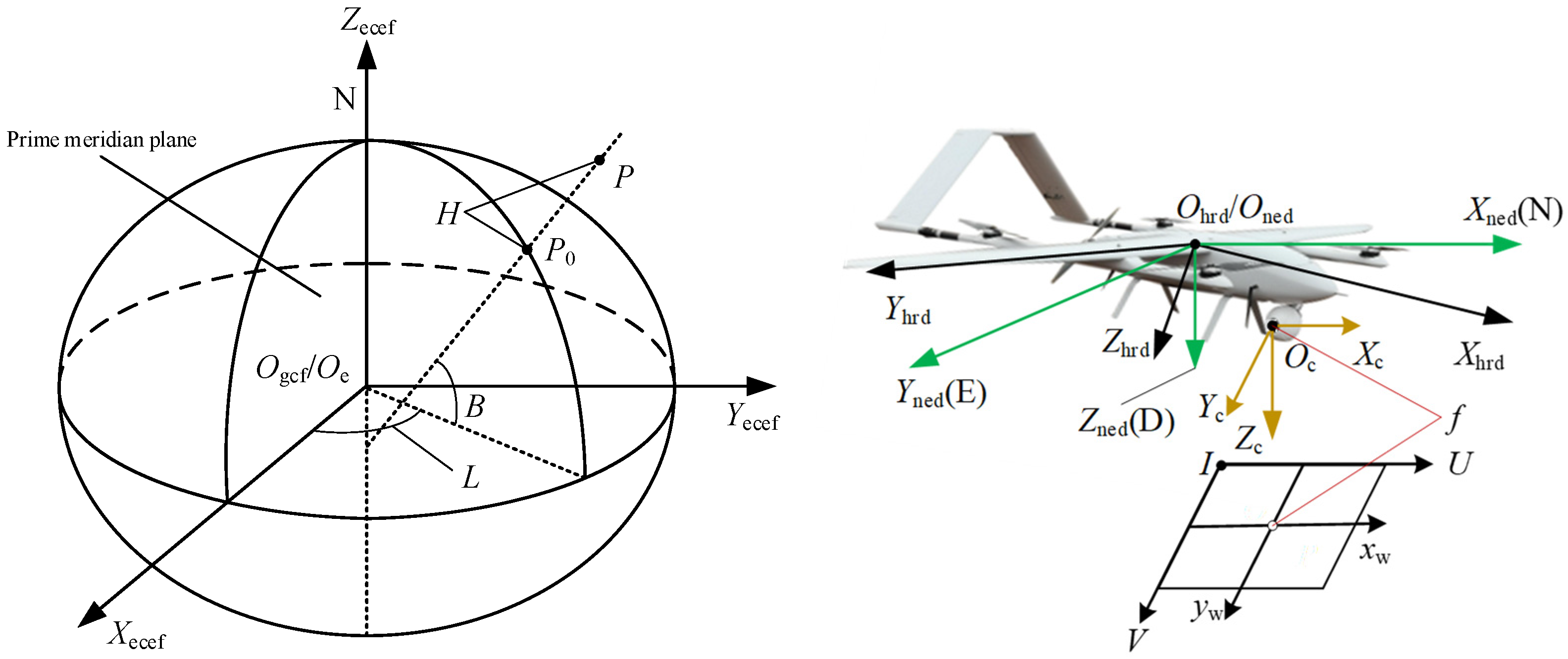
2.1. Base Coordinate System
2.2. Transformation of Coordinate System
3. Error Analysis of Target Localization
3.1. Error Transfer Process
3.2. Synthesis of Errors
4. Assigning Errors Based on Improved Raccoon Optimization Algorithm
4.1. Target Allocation Model
4.2. Raccoon Optimization Algorithm
- (1)
- Exploration phase—cooperative iguana hunting
- (2)
- Development phase—dispersal to escape from predators
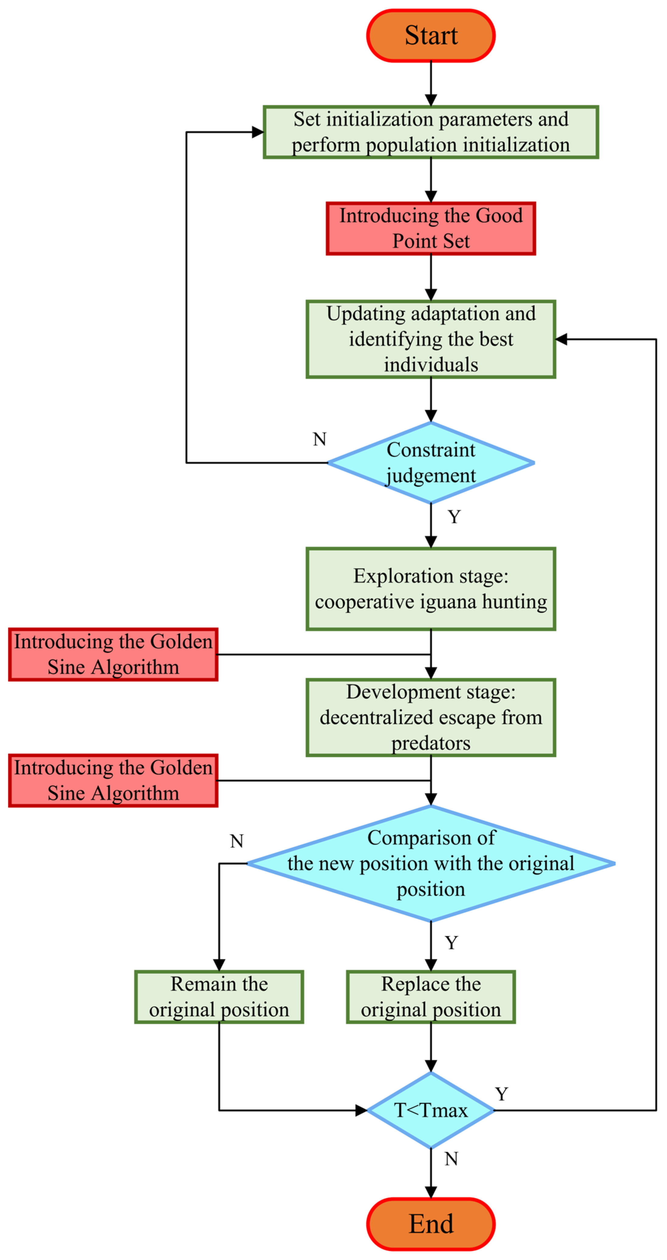
4.3. Improved Raccoon Optimization Algorithm
| Algorithm 1. KYCOA |
| Input: N (coati size), T (number of iterations), ub (upper variable limits), lb (lower variable limits), dim (variable dimensions) F = initialize(N) (Introduce good point set initialization) Updating adaptation and identifying the best individuals While T ≤ Tmax do Update location of the iguana based on best member location Phase 1 for i = 1 to N/2 do Calculate new position for i-th coati using Equation (23) end for for i = N/2 + 1 to N do Calculate random position for the iguana using Equation (24) Introducing the golden sine algorithm Update position of i-th coati using Equation (32) end for Phase 2 for i = 1 to N do Calculate new position for i-th coati using Equation (25) Introducing the golden sine algorithm Update position of i-th coati using Equation (33) end for Comparison of the new position with the original position T = T + 1 end while Output the best solution End |
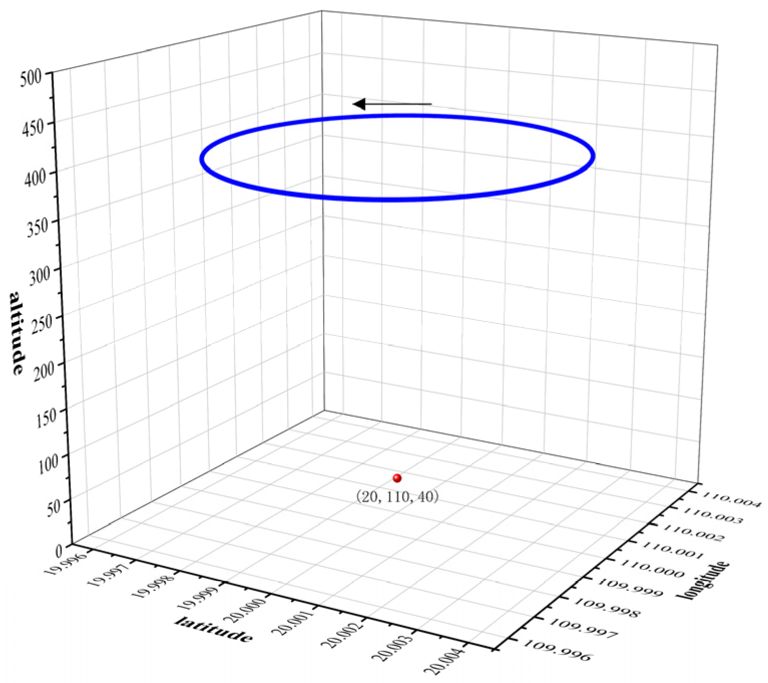
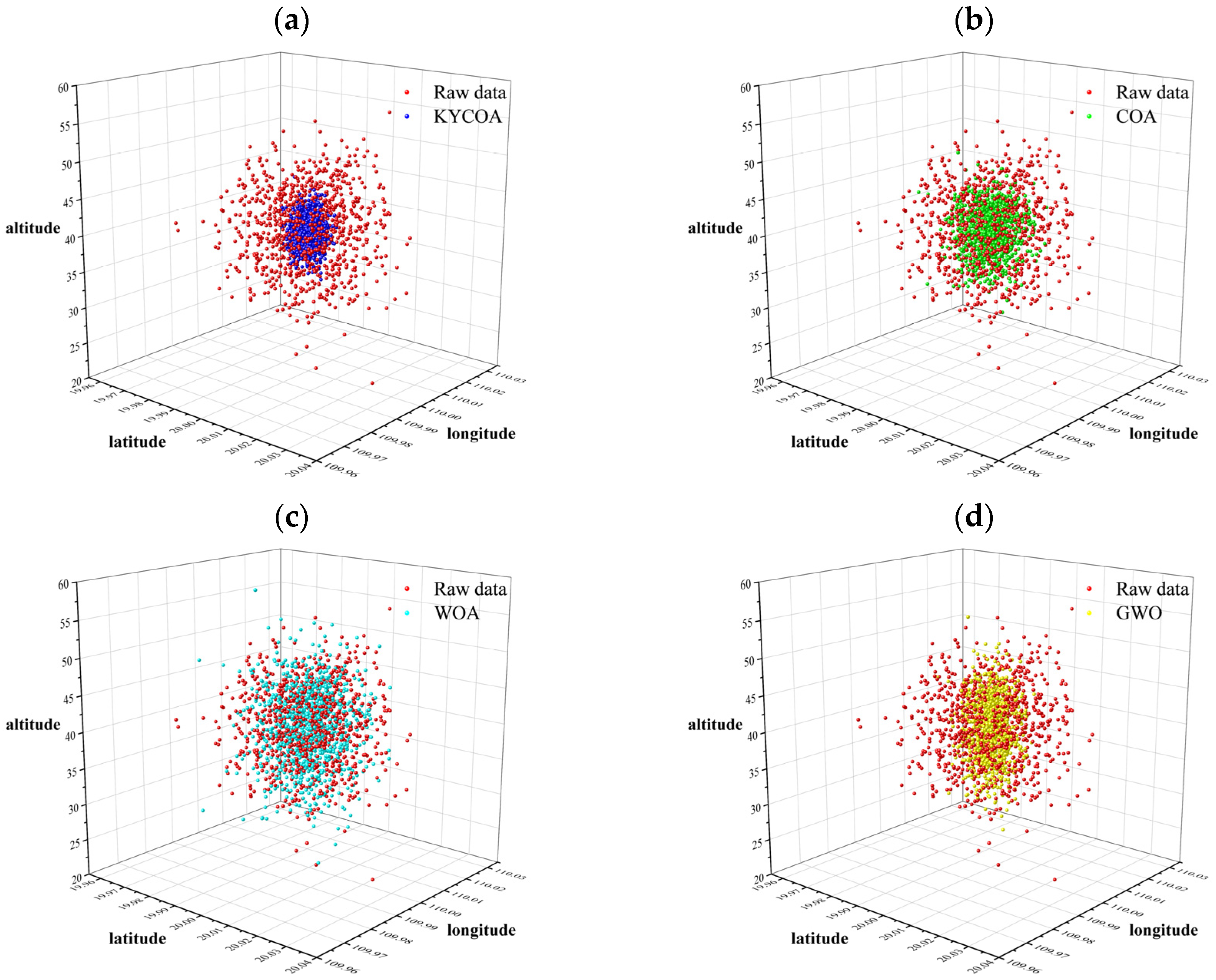
5. Simulation Experiment
6. Actual Flight Test
7. Conclusions
Author Contributions
Funding
Institutional Review Board Statement
Informed Consent Statement
Data Availability Statement
Conflicts of Interest
References
- Wang, X.; Liu, J.; Zhou, Q. Real-Time Multi-Target Localization from Unmanned Aerial Vehicles. Sensors 2017, 17, 33. [Google Scholar] [CrossRef]
- Du, M.; Zou, H.; Wang, T.; Zhu, K. A Cooperative Target Localization Method Based on UAV Aerial Images. Aerospace 2023, 10, 943. [Google Scholar] [CrossRef]
- Kang, X.; Shao, Y.; Bai, G.; Sun, H.; Zhang, T.; Wang, D. Dual-UAV Collaborative High-Precision Passive Localization Method Based on Optoelectronic Platform. Drones 2023, 7, 646. [Google Scholar] [CrossRef]
- Qian, M.; Chen, W.; Sun, R. A Maneuvering Target Tracking Algorithm Based on Cooperative Localization of Multi-UAVs With Bearing-Only Measurements. IEEE Trans. Instrum. Meas. 2024, 73, 9516911. [Google Scholar] [CrossRef]
- Sheng, L.; Li, H.; Qi, Y.; Shi, M. Real Time Screening and Trajectory Optimization of UAVs in Cluster Based on Improved Particle Swarm Optimization Algorithm. IEEE Access 2023, 11, 81838–81851. [Google Scholar] [CrossRef]
- He, L.; Gong, P.; Zhang, X.; Wang, Z. The Bearing-Only Target localization via the Single UAV: Asymptotically Unbiased Closed-Form Solution and Path Planning. IEEE Access 2019, 7, 153592–153604. [Google Scholar] [CrossRef]
- Yan, X.; Zhu, H.; Sun, S.; Shi, Z.; Jiang, S. UAV target localization method based on improved variant firefly optimized particle filtering. J. Mil. Eng. 2024, 1–13. [Google Scholar]
- Wang, Y.; Li, H.; Li, X.; Wang, Z.; Zhang, B. UAV image target localization method based on outlier filter and frame buffer. Chin. J. Aeronaut. 2024, 37, 375–390. [Google Scholar] [CrossRef]
- Zhou, Y.; Song, D.; Ding, B.; Rao, B.; Su, M.; Wang, W. Ant Colony Pheromone Mechanism-Based Passive Localization Using UAV Swarm. Remote Sens. 2022, 14, 2944. [Google Scholar] [CrossRef]
- Du, Y.; Ding, Y.; Xu, Y.; Liu, Z.; Xiu, J. Algorithm for ground target localization by TDI-CCD panoramic aerial camera. J. Opt. 2017, 37, 355–365. [Google Scholar]
- Gong, W.; Lou, S.; Deng, L.; Yi, P.; Hong, Y. Efficient Multi-Target Localization Using Dynamic UAV Clusters. Sensors 2025, 25, 2857. [Google Scholar] [CrossRef]
- Tan, L.; Cheng, Q.; Wei, M.; Li, J.; Luo, W. Passive localization and error analysis of single station for surface target optronics. Appl. Opt. 2024, 45, 673–684. [Google Scholar]
- Ren, H.; Huang, C.; Wang, S.; Wang, D.; Ren, Z. A Method for Target Positioning Calculation and Error Analysis of an Unmanned Aerial Vehicle Electro-Optical Pod. China Plant Eng. 2020, 22, 128–131. [Google Scholar]
- Yarima, S.I.; Sha’ameri, A.Z.; Yaro, A.S. Analysis of condition number and position estimation error for multiangulationposition estimation system. Turk. J. Electr. Eng. Comput. Sci. 2020, 28, 1503–1518. [Google Scholar] [CrossRef]
- Liu, S.; Lin, Z.; Feng, R.; Huang, W.; Yan, B. Intelligent control method for automatic voltage regulator: An improved coati optimization algorithm-based strategy. Measurement 2025, 252, 117263. [Google Scholar] [CrossRef]
- Gopal, A.; Sultani, M.M.; Bansal, J.C. On Stability Analysis of Particle Swarm Optimization Algorithm. Arab. J. Sci. Eng. 2020, 45, 2385–2394. [Google Scholar] [CrossRef]
- Liu, Z.; Hou, J.; Ning, D.; Zhang, F.; Liang, G. Rescue plan of unmanned life-saving vehicle in multi-obstacle waters under multi-strategy innovative ant colony optimization strategy. Ocean. Eng. 2025, 331, 121242. [Google Scholar] [CrossRef]
- Li, L.; Liu, L.; Shao, Y.; Zhang, X.; Chen, Y.; Guo, C.; Nian, H. Enhancing Swarm Intelligence for Obstacle Avoidance with Multi-Strategy and Improved Dung Beetle Optimization Algorithm in Mobile Robot Navigation. Electronics 2023, 12, 4462. [Google Scholar] [CrossRef]
- Dehghani, M.; Montazeri, Z.; Trojovská, E.; Trojovský, P. Coati Optimization Algorithm: A new bio-inspired metaheuristic algorithm for solving optimization problems. Knowl. Based Syst. 2023, 259, 110011. [Google Scholar] [CrossRef]
- Deng, W.; Mo, Y.; Deng, L. A Multimodal Multi-Objective Coati Optimization Algorithm Based on Spectral Clustering. Symmetry 2024, 16, 1474. [Google Scholar] [CrossRef]
- Jia, C.; He, L.; Liu, D.; Fu, S. Path planning and engineering problems of 3D UAV based on adaptive coati optimization algorithm. Sci. Rep. 2024, 14, 30717. [Google Scholar] [CrossRef] [PubMed]
- Adam, S.P.; Alexandropoulos, S.-A.N.; Pardalos, P.M.; Vrahatis, M.N. No free lunch theorem: A review. In Approximation and Optimization; Springer: Cham, Switzerland, 2019; Volume 145, pp. 57–82. [Google Scholar]
- Zhou, X.; Cheng, Y.; Qiao, D.; Huo, Z. An adaptive surrogate model-based fast planning for swarm safe migration along halo orbit. Acta Astronaut. 2022, 194, 309–322. [Google Scholar] [CrossRef]
- Peng, H.; Wang, W. Adaptive surrogate model-based fast path planning for spacecraft formation reconfiguration on libration point orbits. Aerosp. Sci. Technol. 2016, 54, 151–163. [Google Scholar] [CrossRef]
- Wang, J.; Wu, W. Target Tracking Technology for Moving Sensors; National Defense Industry Press: Beijing, China, 2017. [Google Scholar]
- Zhou, X.; Jia, W.; He, R.; Sun, W. High-Precision Localization Tracking and Motion State Estimation of Ground-Based Moving Target Utilizing Unmanned Aerial Vehicle High-Altitude Reconnaissance. Remote Sens. 2025, 17, 735. [Google Scholar] [CrossRef]
- Liu, X.; Zhang, Z. A Vision-Based Target Detection, Tracking, and Positioning Algorithm for Unmanned Aerial Vehicle. Wirel. Commun. Mob. Comput. 2021, 2021, 5565589. [Google Scholar] [CrossRef]
- Xu, C.; Yin, C.; Han, W.; Wang, D. Two-UAV trajectory planning for cooperative target locating based on airborne visual tracking platform. Electron. Lett. 2020, 56, 301–303. [Google Scholar] [CrossRef]
- Mu, S.; Qiao, C. Ground-target geo-location method based on extended Kalman filtering for small-scale airborne electrooptical platform. Acta Opt. Sin. 2019, 39, 321–331. [Google Scholar]
- Jiang, Y.; Li, N.; Gong, X.; Jia, G.; Zhao, H. Improved Position Error Model for Airborne Hyperspectral Imaging Systems. Int. J. Pattern Recognit. Artif. Intell. 2019, 30, 1954017. [Google Scholar] [CrossRef]
- Bai, G.; Liu, J.; Song, Y.; Zuo, Y. Two-UAV Intersection Localization System Based on the Airborne Optoelectronic Platform. Sensors 2017, 17, 98. [Google Scholar] [CrossRef]


| Parameters | Symbol | Standard Deviation | Value |
|---|---|---|---|
| UAV Latitude | 0.0001 | ||
| UAV Longitude | 0.0001 | ||
| UAV Height | 5 | 400 m | |
| UAV Yaw Angle | 0.2 | \ | |
| UAV Pitch Angle | 0.2 | 0 | |
| UAV Roll Angle | 0.2 | ||
| Pod Heading Angle | 2 | ||
| Pod Pitch Angle | 2 |
| Truth Value | Raw Data | KYCOA | COA | WOA | GWO | |
|---|---|---|---|---|---|---|
| Latitude\° | 20 | 19.999633 | 19.999881 | 19.999791 | 19.999679 | 19.999832 |
| Longitude\° | 110 | 110.000011 | 109.999971 | 109.999977 | 109.999976 | 110.000018 |
| Altitude\m | 40 | 40.275 | 39.995 | 39.993 | 39.988 | 39.990 |
| Distance\m | 0 | 40.825 | 13.575 | 23.364 | 35.782 | 18.775 |
| Raw Data | KYCOA | COA | WOA | GWO | |
|---|---|---|---|---|---|
| Latitude\° | 0.24703 | 0.064617 | 0.10842 | 0.17047 | 0.082745 |
| Longitude\° | 0.24253 | 0.064714 | 0.11059 | 0.17178 | 0.085314 |
| Altitude\° | 126.19 | 52.16 | 78.24 | 130.4 | 104.32 |
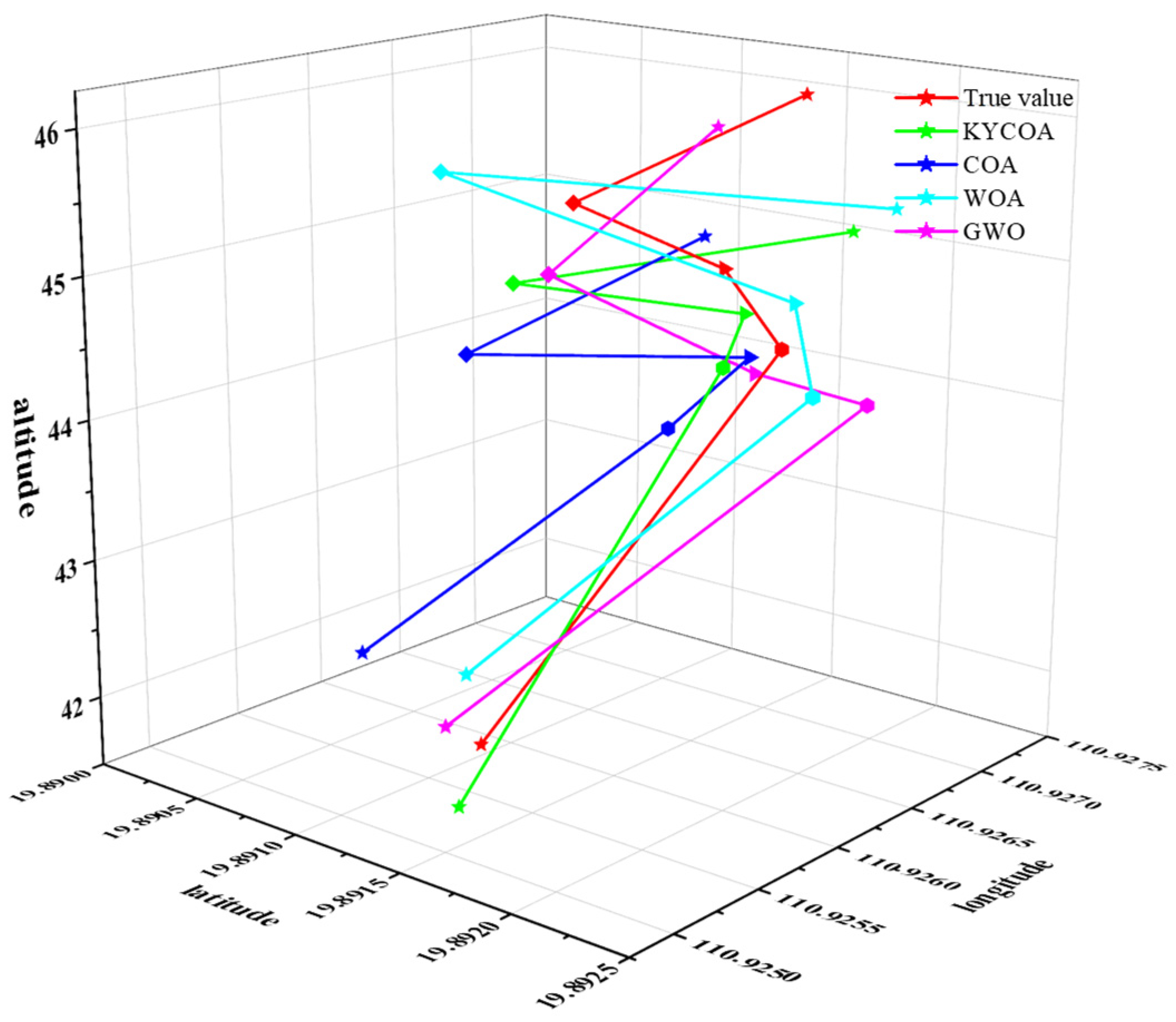
| Target Point | Latitude (°) | Longitude (°) | Altitude (°) |
|---|---|---|---|
| target point 1 | 19.89147036 | 110.9267209 | 44.8845 |
| target point 2 | 19.89178402 | 110.9266519 | 44.4267 |
| target point 3 | 19.89154581 | 110.9271469 | 46.0313 |
| target point 4 | 19.89066431 | 110.9268279 | 45.1168 |
| target point 5 | 19.89125446 | 110.9255049 | 41.8700 |
| Target Point | KYCOA (m) | COA (m) | WOA (m) | GWO (m) |
|---|---|---|---|---|
| target point 1 | 22.14 | 39.34 | 50.66 | 33.41 |
| target point 2 | 26.50 | 45.73 | 55.09 | 35.86 |
| target point 3 | 20.60 | 43.63 | 54.85 | 37.20 |
| target point 4 | 27.17 | 47.48 | 57.46 | 40.22 |
| target point 5 | 26.05 | 46.51 | 53.84 | 31.60 |
Disclaimer/Publisher’s Note: The statements, opinions and data contained in all publications are solely those of the individual author(s) and contributor(s) and not of MDPI and/or the editor(s). MDPI and/or the editor(s) disclaim responsibility for any injury to people or property resulting from any ideas, methods, instructions or products referred to in the content. |
© 2025 by the authors. Licensee MDPI, Basel, Switzerland. This article is an open access article distributed under the terms and conditions of the Creative Commons Attribution (CC BY) license (https://creativecommons.org/licenses/by/4.0/).
Share and Cite
Li, Y.; Hu, Q.; Sun, S.; Ying, W.; Yan, X. Research on Nonlinear Error Compensation and Intelligent Optimization Method for UAV Target Positioning. Sensors 2025, 25, 4340. https://doi.org/10.3390/s25144340
Li Y, Hu Q, Sun S, Ying W, Yan X. Research on Nonlinear Error Compensation and Intelligent Optimization Method for UAV Target Positioning. Sensors. 2025; 25(14):4340. https://doi.org/10.3390/s25144340
Chicago/Turabian StyleLi, Yinglei, Qingping Hu, Shiyan Sun, Wenjian Ying, and Xiaojia Yan. 2025. "Research on Nonlinear Error Compensation and Intelligent Optimization Method for UAV Target Positioning" Sensors 25, no. 14: 4340. https://doi.org/10.3390/s25144340
APA StyleLi, Y., Hu, Q., Sun, S., Ying, W., & Yan, X. (2025). Research on Nonlinear Error Compensation and Intelligent Optimization Method for UAV Target Positioning. Sensors, 25(14), 4340. https://doi.org/10.3390/s25144340