
Investigating a Machine Learning Approach to Predicting White Pixel Defects in Wafers—A Case Study of Wafer Fabrication Plant F


Abstract
1. Introduction
2. Preliminary
2.1. White Pixel Defects
2.2. Machine Learning Approach
- Machine learning models can process large amounts of image data (such as semiconductor wafer scans) faster than manual inspection methods or traditional automated methods that rely on simpler algorithms. Once trained, these models can analyze new imagery almost instantly, which is critical to maintaining production line speeds and meeting high demand.
- Machine learning models are able to learn from data and improve over time without being explicitly programmed for each specific task. This means they can become more efficient and accurate as more data are processed.
- The automation provided by machine learning reduces the need for human input during the inspection process, allowing for continuous operations without the interruptions or slowdowns typically seen with manual inspections, and reducing the potential for human error.
- Machine learning systems can easily scale as production volumes increase and can easily adapt to different types of defects or changes in the manufacturing process. Traditional methods may require significant reconfiguration or redevelopment to handle new types of defects or changes in the manufacturing environment.
- Machine learning models can be integrated into existing quality control systems to enhance their functionality rather than completely replacing them. This integration can significantly increase speed and efficiency because these models enhance the capabilities of traditional methods by adding layers of intelligence and adaptability.
- In addition to detecting existing defects, machine learning models can predict potential future failures by identifying subtle patterns that may precede defects. This saves a lot of time and resources.
2.2.1. Decision Tree (C5.0)
2.2.2. CART
2.2.3. Random Forest
2.2.4. Support Vector Machine
3. Methodology
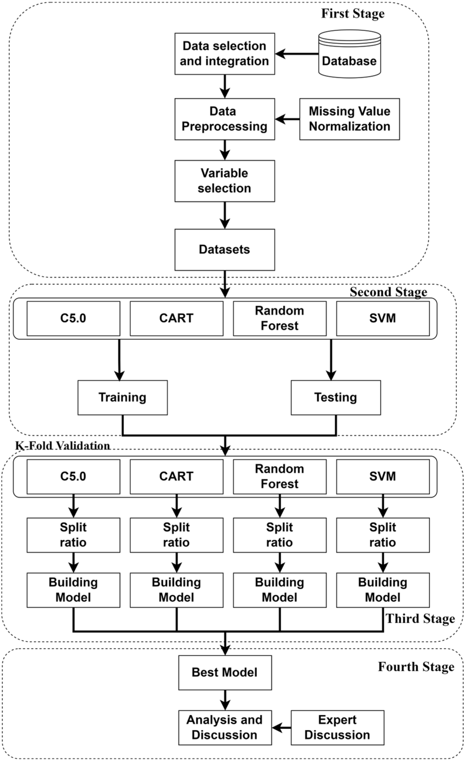
3.1. Framework
- First Stage—Data Selection and Integration: This stage involves outlining the data sources utilized in the study, along with a description of how the collected data are processed and formatted to meet the study’s requirements. It includes defining the research dependent and independent variables. Data pre-processing: here, the study addresses noise reduction, elimination of incomplete data, and normalization techniques to enhance the accuracy of the predictive model. Research variable screening: the methodology for variable selection is explained, including the use of a multinomial logit regression algorithm in R to identify significant factors influencing white pixel defects, resulting in the construction of the input model with 45 relevant variables.
- Second Stage: At this stage, the basic model of machine learning is selected. The choice between basic machine learning models and deep learning models depends on the specific requirements of the task, including the need for interpretability, dataset characteristics, computational resources, and expertise. For white pixel defect prediction, the advantages of basic models in terms of interpretability, efficiency, and performance on structured data make them appealing choices for initial exploration and analysis. Therefore, C5.0 and CART, along with random forest and SVM, are selected to further the investigation.
- Third Stage: In this stage, the analyzed data are employed for model construction and prediction procedures. The K-fold cross-validation method is employed to identify the most accurate prediction model.
- Fourth Stage: To compare and evaluate the R language-constructed models, the study fixes the seed setting value at 123 in R for consistency across calculations. The decision tree (C5.0), CART, RF, and SVM models are constructed and compared. The best-performing prediction model is revealed. Furthermore, significant factors obtained from models are extracted and analyzed for their impact on white pixel defects.
3.2. Case Study
- Step 1: Gather 4980 pieces of Company F’s process data and customer complaint pixel data, focusing on significant periods for analysis.
- Step 2: Define model variables. Following discussions with senior engineers specializing in wafer manufacturing technology, the research scope was confined to the wafer surface grinding process. The aim was to identify input variables potentially affecting white pixel defects in CIS products.
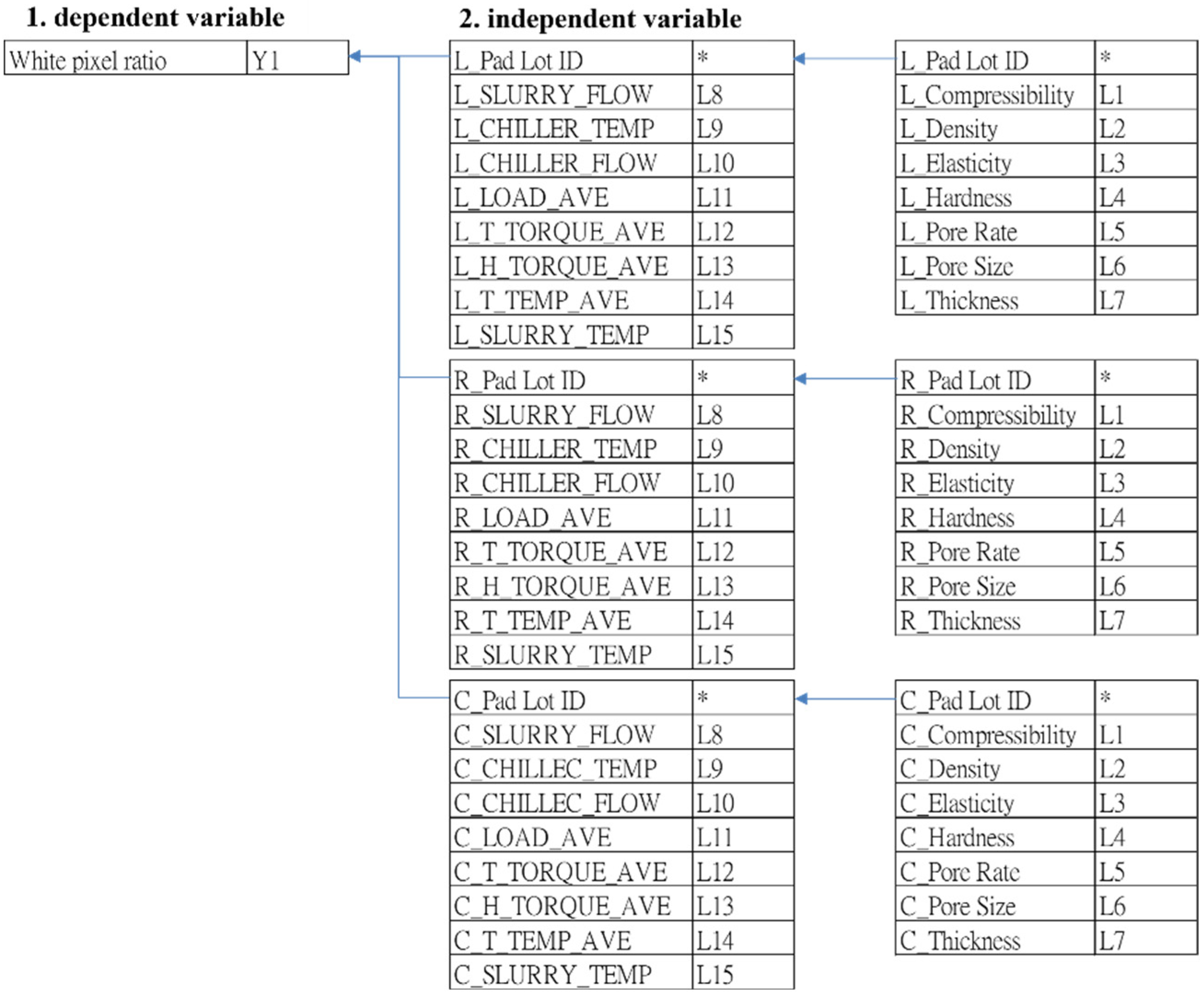
- Step 3: Screen processing variables of the grinding process. The grinding mechanism comprises three programs: R, C, and L. Within the wafer mirror grinding process, the R program aims to eliminate grinding stress and remove oxide film, while the C and L programs aim to enhance surface roughness and particle levels. The RCL program revealed 45 influencing variables, each described in Table 3, with their interrelations and correlations depicted in Figure 7.
- Step 4: Data pre-processing. After confirming the research range of the collected case data and deleting missing data and duplicate data.
Data Collection and Pre-Processing
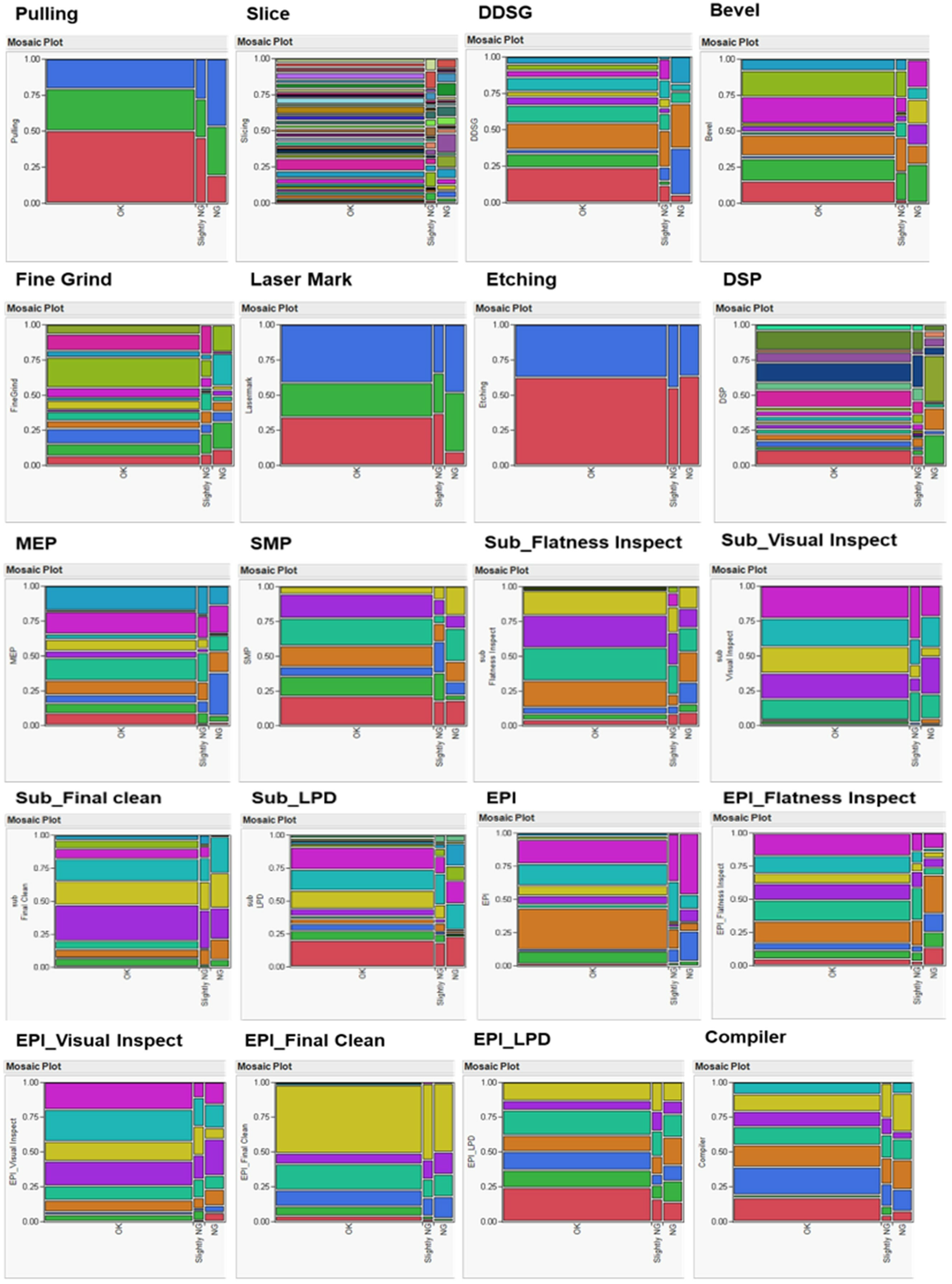
- Data Attributes: The data collection for this study revolves around information concerning the pad of Company F’s grinding equipment. The primary focus is on predicting its degree of influence on white pixels, serving as the dependent variable. This determination is based on the processing conditions of the grinding equipment and the material certificate of analysis (COA) information. The white pixel result information provided by Company F’s customers is categorized into groups, as outlined in Table 4. It is classified into two levels: ‘OK’ indicating good products and ‘NG’ indicating seriously defective ones.
- Variable Selection: The select variables in this study involved consultations with senior engineers from Company F. All polishing engineering variables potentially impacting the white pixel problem were chosen based on the processing conditions of the individual wafer manufacturing plant. The suggested items are detailed in Table 5, comprising a total of 45 variables utilized as initial input variables.
3.3. Data Preprocessing
- Handling Incomplete or Noisy Data: It is common to encounter missing fields or incomplete data within a dataset. To address this, one approach is to outright delete the entries or to replace them with the average value of the dataset. Alternatively, setting missing values to a null state allows for their exclusion from analysis.
- Data Normalization: To ensure that the dataset aligns with the requirements of the predictive algorithm, it must undergo normalization. This process adjusts input and output variables to fit within a specific range, often called scaling. After model training, the output values produced during inference need to be rescaled back to their original range. This study employs interval mapping for scaling, adjusting the data variables’ minimum and maximum values to align with the desired range. As a result of normalization, all input values are scaled to fall between 0 and 1.
3.4. K-Fold Cross-Validation
3.5. Evaluation Metrics
- (1)
- Accuracy
- (2)
- Precision
- (3)
- Specificity
- (4)
- F-Score
4. Experimental Results and Analysis
- Hardware: Powerful CPU (Intel i9), high-performance GPU (NVIDIA RTX 3080), ample RAM (32 GB). Fast solid-state drive (NVMe SSD).
- Software: GUI and compatibility for the operating system Windows. Programming language: scikit-learn, R4.3. Scikit-Learn 1.4 for general machine learning. Git is used for source code management. GitHub online code repository and collaboration.
- This comprehensive environment supports a wide range of machine learning activities from data preprocessing and model training to deployment and monitoring, ensuring experiments can run efficiently and effectively.
- It is a common practice to use default parameter values when comparing multiple machine learning models, especially in the initial stages of model evaluation. There are usually several reasons for this approach:
- Default parameters provide baseline performance for each model. This allows you to immediately see the performance of each algorithm without making any adjustments. This is a quick way to measure how well a model suits a particular type of data or problem.
- Using default settings, all models start on a level playing field. This fairness is crucial when your goal is to compare different types of models to understand which model inherently fits the material better and is not subject to extensive parameter optimization.
- Use preset parameters to make your experiments more reproducible. Other researchers can easily validate your results by using the same model with default settings, ensuring that performance metrics are attributed to the model itself and not to specific adjustments made to it.
4.1. Sample
4.2. Variable Selection and Results
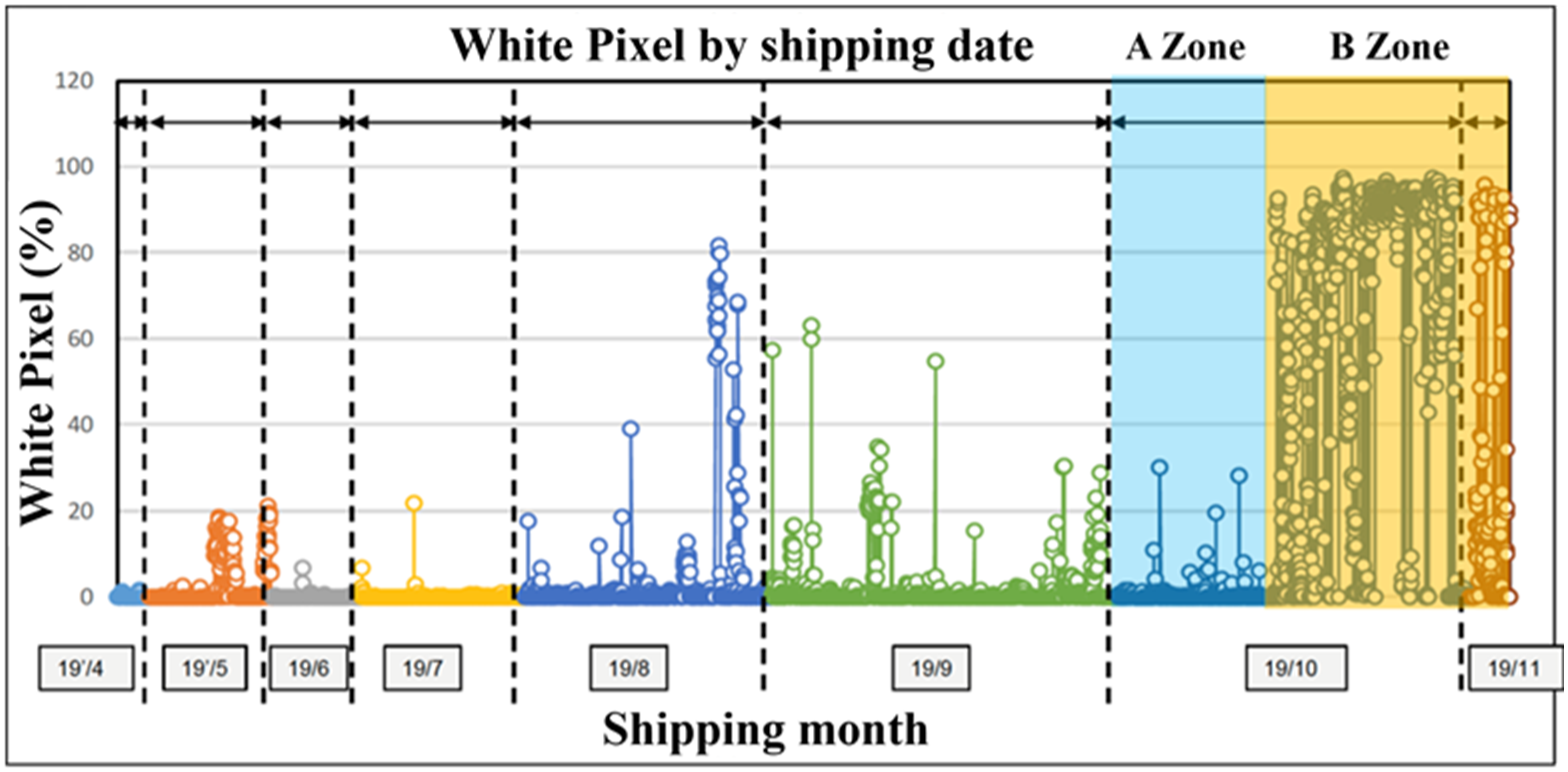
- Screening Variables in the A Zone (Count: 1152): The investigation utilized 45 variables, recommended for assessing the processing conditions within a semiconductor wafer manufacturing facility. These variables served as input factors for conducting a screening process. Utilizing the logistic regression algorithm [20], implemented in R programming language, the study aimed to identify variables significantly influencing the occurrence of white pixel defects. The analysis, focusing on the period before the notable rise in white pixel defects (A Zone), revealed that six variables significantly impact the incidence of these defects. These variables are distributed across three axes: two significant variables on the L-axis, two on the R-axis, and two on the C-axis, as detailed in Table 6.
- Variable screening in the B Zone: In the B Zone (Count: 910, where a large number of white pixel defects occur), 27 significant items of variable (L-axis: 7 items, R-axis: 11 items, C-axis: 9 items) were found, as shown in Table 7.
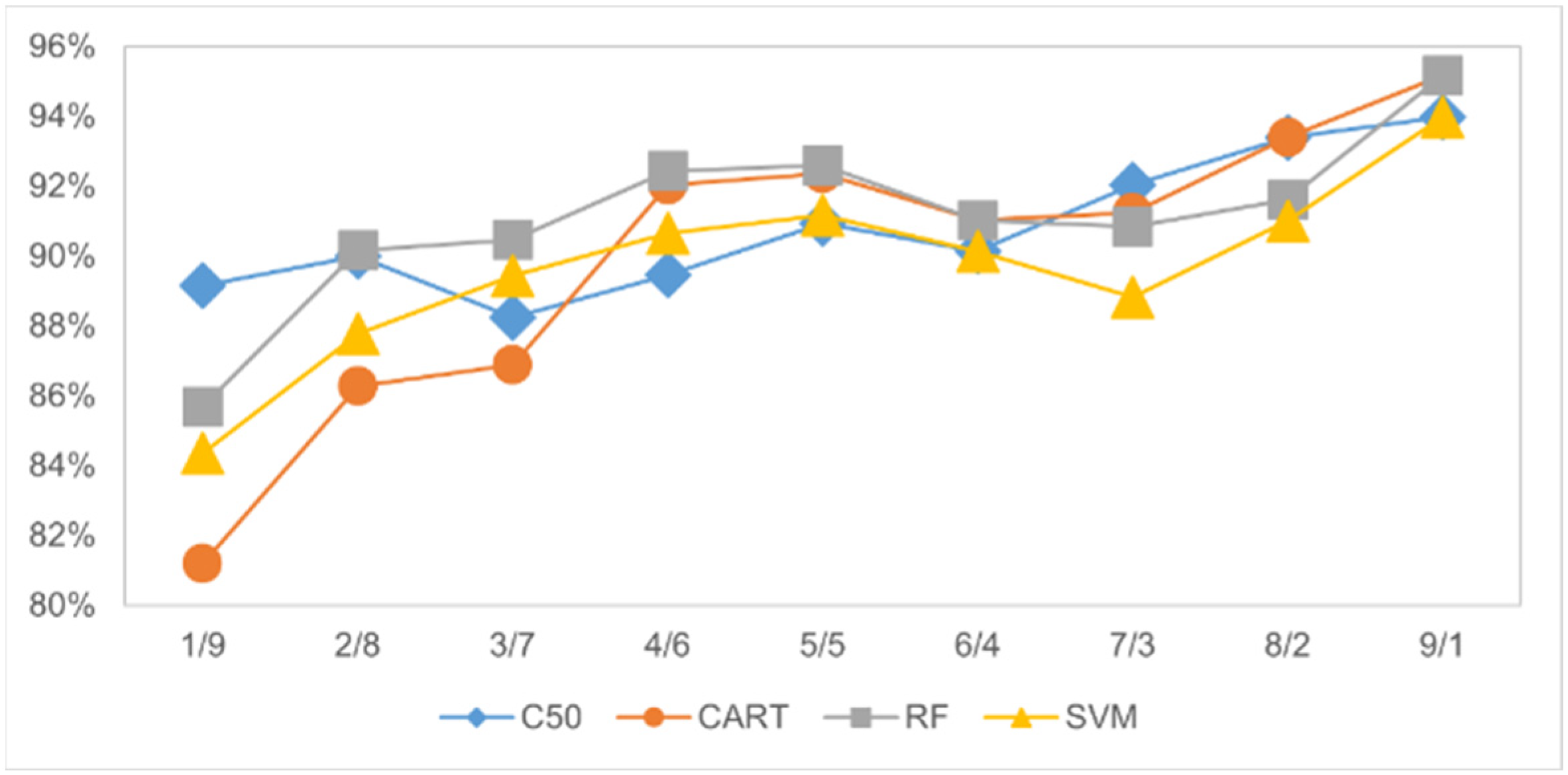
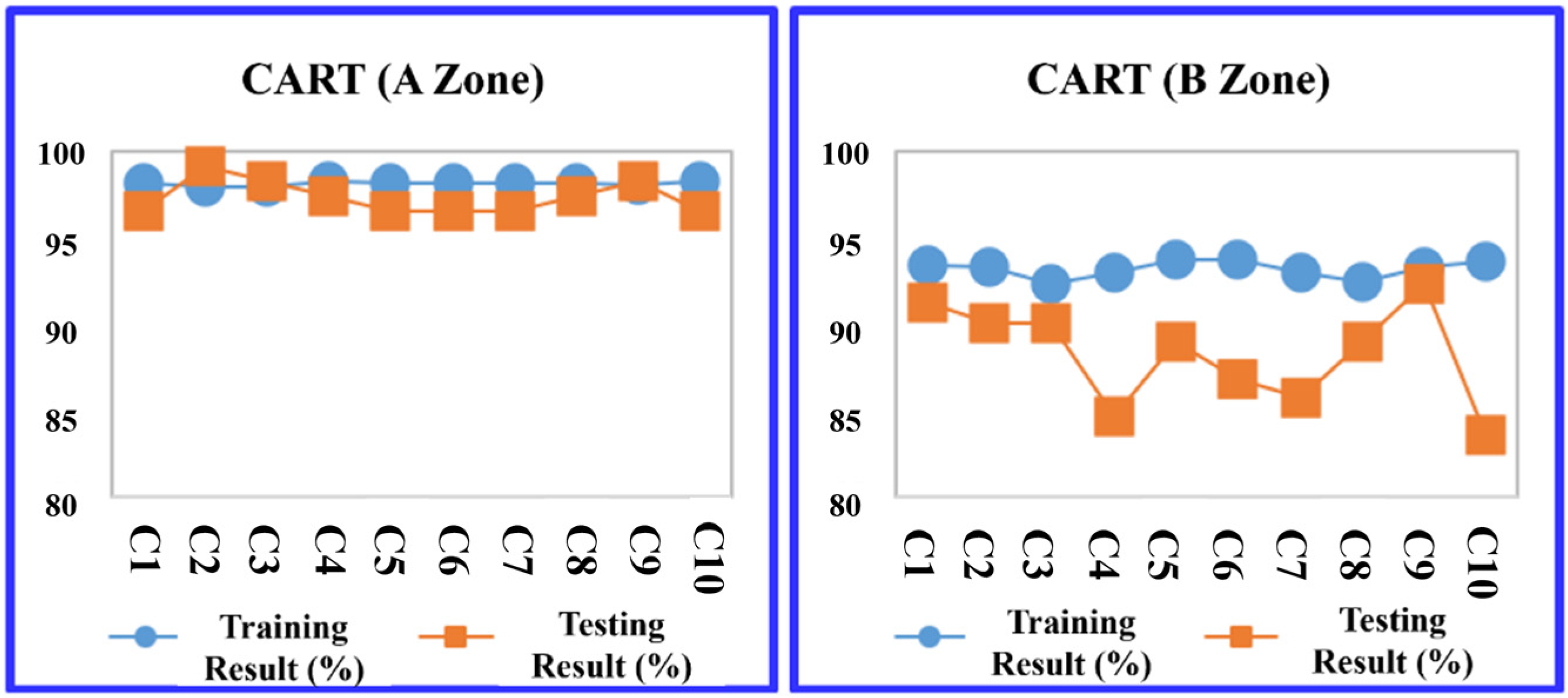
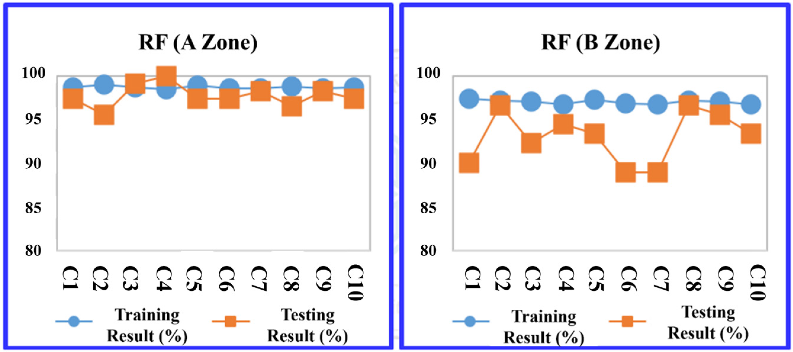
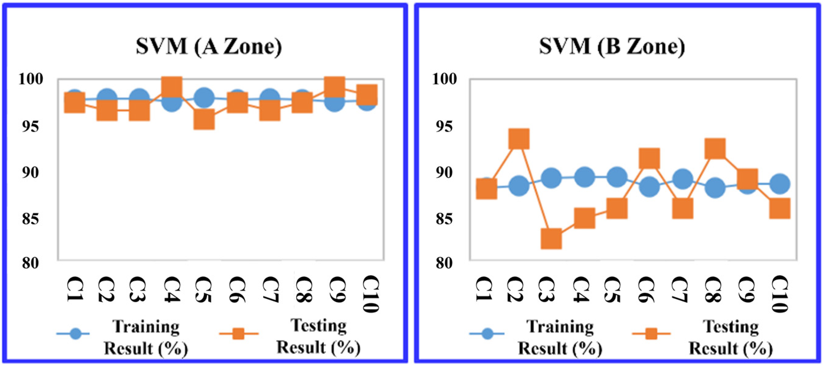
4.3. Comparison of Prediction Models for the A and B Zones
4.4. Prediction Rule Extraction and Factors Discussion
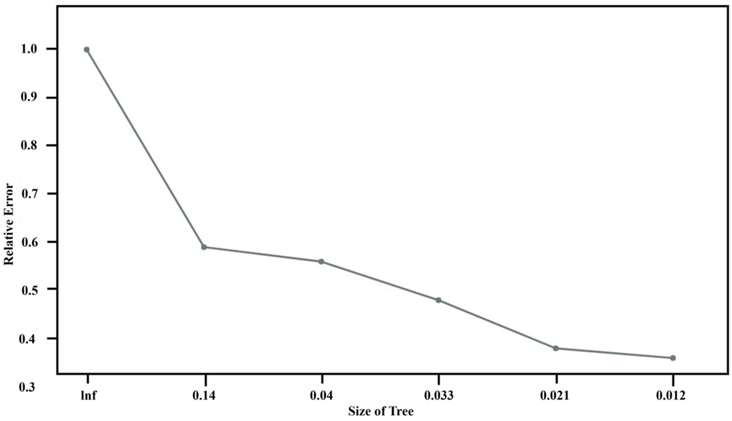
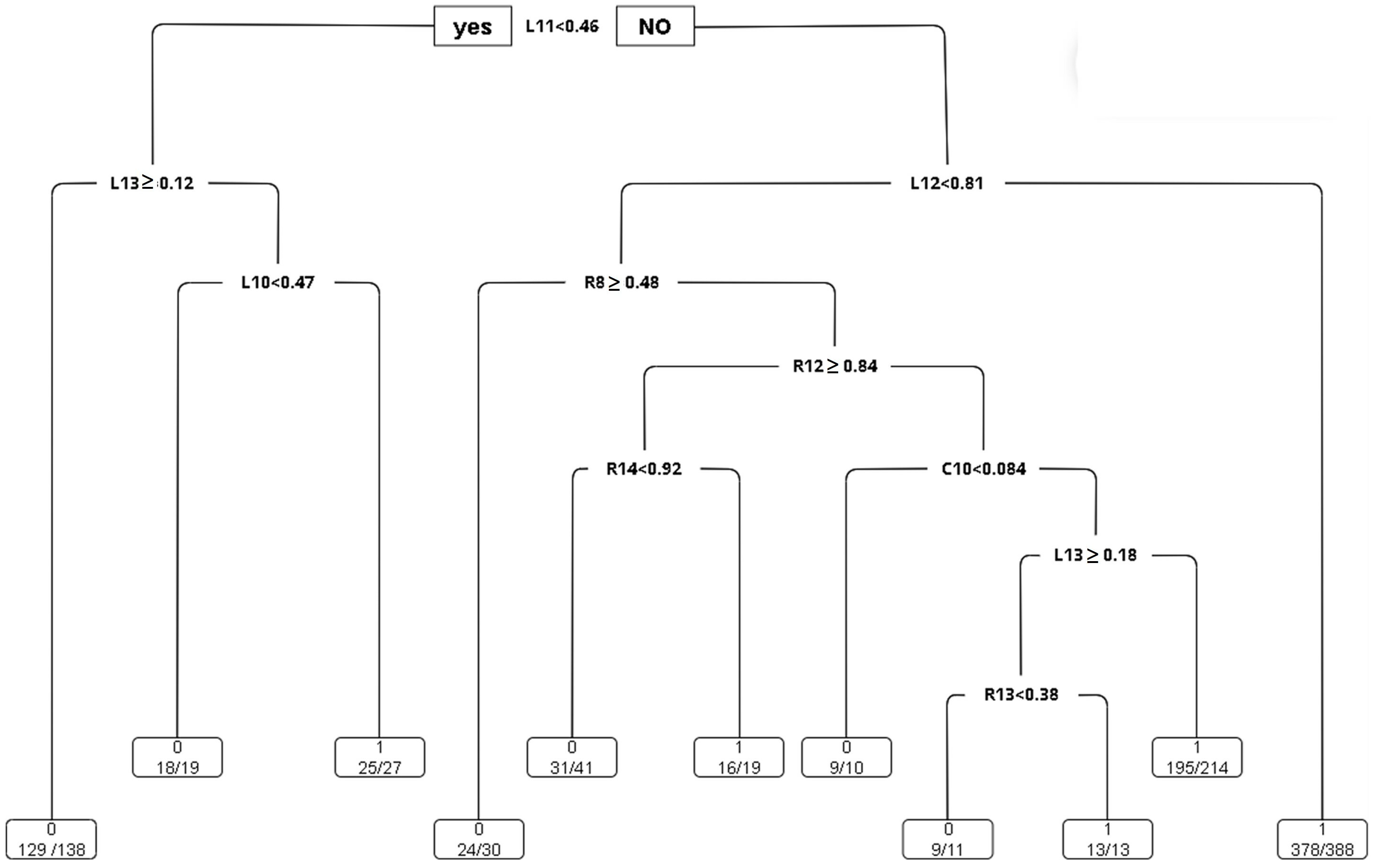
- CART: The study employs the CART algorithm for the development of a decision tree model, as illustrated in Figure 15. An analysis of the complexity parameters and error rates for the unpruned CART decision tree model post-training reveals insights into the model’s error dynamics. As demonstrated in Figure 16, the model achieves its minimum cross-validation error of 0.013780 when the tree is configured with nine leaf nodes (indicating eight splits).
- 2.
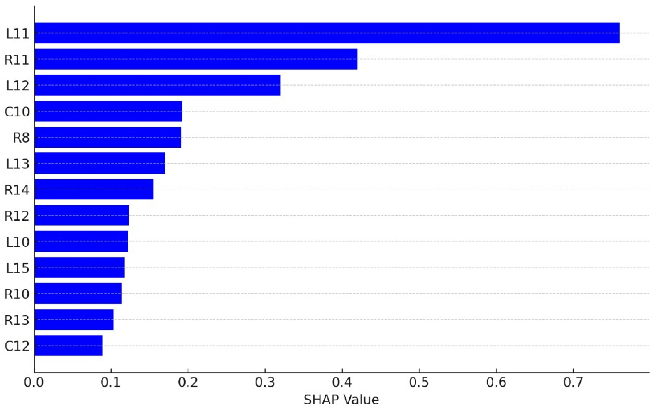
- RF: The mean decrease Gini coefficient, often referred to in the context of random forest and other tree-based models, measures the importance of a feature (variable) in a predictive model. A higher mean decrease Gini indicates that a feature more effectively splits the dataset into groups with similar outcomes, thus being more important for the prediction. The trained random forest model can measure the importance of variables through the mean decrease Gini coefficient. The data show that variable L11 is the most important feature, followed by R11, L12, C10, R8, L13, and R14.
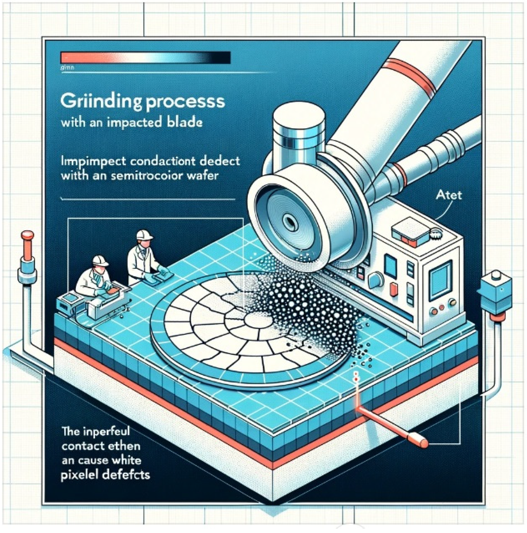
- Mechanical Stress: Grinding involves applying mechanical stress to thin the wafer to the desired thickness. An excessive load during this process can induce micro-cracks and subsurface damage, which may not be visible immediately but can manifest as white pixel defects later in the manufacturing process or during the operation of the final semiconductor device.
- Heat Generation: Grinding generates heat due to friction between the wafer and the grinding wheel. High grinding loads increase this heat generation, potentially causing local overheating. This can lead to slip dislocations, changes in material properties, or other forms of damage at a microscopic level, contributing to defect formation.
- Surface Quality Degradation: The quality of the wafer surface post-grinding is crucial for subsequent manufacturing steps, such as lithography. High grinding loads can degrade surface quality by introducing roughness, pits, and scratches. These surface irregularities can interfere with subsequent processes, leading to defects, including white pixels, in the finished product.
- Impurities and Contamination: The grinding process, especially under high loads, can lead to the embedding of abrasive particles or the generation of debris that becomes embedded in the wafer surface. These impurities can act as nucleation sites for defects.
- Non-uniform Material Removal: Ideally, grinding should remove material uniformly across the wafer. However, excessive or unevenly distributed grinding loads can lead to non-uniform thickness, warping, or localized thinning, which may result in stress concentrations. These stress concentrations can manifest as white pixel defects during further processing or in the final product.
5. Conclusions
5.1. Findings
- Loadbearing (L11, R11) and torque (C10, L12, L13, R12) during the wafer manufacturing process are identified as key elements. The study indicates a direct relationship between the grinding machinery’s applied load and torque and the probability of causing wafer surface damage, which subsequently increases the risk of white pixel defects. This damage aids in the adherence of external contaminants on the wafer surface, which subsequent cleaning processes may not fully remove. These contaminants, if left on the wafer surface, can infiltrate deeper layers during thermal processing, potentially culminating in white pixel defects in the final product.
- The study delineates two essential rules for predicting white pixel defects:
- A higher likelihood of white pixel defects occurs when the SMP L-axis load value meets or exceeds 0.46 and the L-axis Table torque value meets or exceeds 0.81, with the CART model showcasing a 97% accuracy rate in this prediction.
- Conversely, the probability of white pixel defects markedly decreases when the SMP L-axis load value is less than 0.46, the L-axis chill flow is below 0.47, and the L-axis head table torque value is under 0.12.
- The analysis further reveals that the most critical factors predominantly pertain to the L-axis, consistent with Company F’s observations. The significant presence of white pixel defects was linked to the L-axis of the SMP grinding equipment, particularly associated with using a specific batch of pads and certain grinding parameters. These factors, related to both the equipment and materials used, were identified as the primary contributors to the notable occurrence of white pixel defects.
5.2. Suggestion and Future Study
Author Contributions
Funding
Institutional Review Board Statement
Data Availability Statement
Conflicts of Interest
References
- Hamdioui, S.; Taouil, M.; Haron, N.Z. Testing Open Defects in Memristor-Based Memories. IEEE Trans. Comput. 2013, 64, 247–259. [Google Scholar] [CrossRef]
- Li, K.S.M.; Jiang, X.H.; Chen, L.L.Y.; Wang, S.J.; Huang, A.Y.A.; Chen, J.E.; Liang, H.C.; Hsu, C.L. Wafer Defect Pattern Labeling and Recognition Using Semi-Supervised Learning. IEEE Trans. Semicond. Manuf. 2022, 35, 291–299. [Google Scholar] [CrossRef]
- Yu, J.; Liu, J. Two-dimensional principal component analysis-based convolutional autoencoder for wafer map defect detection. IEEE Trans. Ind. Electron. 2020, 68, 8789–8797. [Google Scholar] [CrossRef]
- Chien, J.-C.; Wu, M.-T.; Lee, J.-D. Inspection and Classification of Semiconductor Wafer Surface Defects Using CNN Deep Learning Networks. Appl. Sci. 2020, 10, 5340. [Google Scholar] [CrossRef]
- Ma, J.; Zhang, T.; Yang, C.; Cao, Y.; Xie, L.; Tian, H.; Li, X. Review of Wafer Surface Defect Detection Methods. Electronics 2023, 12, 1787. [Google Scholar] [CrossRef]
- Chen, X.; Chen, J.; Han, X.; Zhao, C.; Zhang, D.; Zhu, K.; Su, Y. A Light-Weighted CNN Model for Wafer Structural Defect Detection. IEEE Access 2020, 8, 24006–24018. [Google Scholar] [CrossRef]
- Kim, T.; Behdinan, K. Advances in Machine Learning and Deep Learning Applications towards Wafer Map Defect Recognition and Classification: A Review. J. Intell. Manuf. 2022, 33, 1805–1826. [Google Scholar] [CrossRef]
- Cheng, K.C.C.; Chen, L.L.Y.; Li, J.W.; Li, K.S.M.; Tsai, N.C.Y.; Wang, S.J.; Huang, A.Y.A.; Chou, L.; Lee, C.S.; Chen, J.E.; et al. Machine learning-based detection method for wafer test induced defects. IEEE Trans. Semicond. Manuf. 2021, 34, 161–167. [Google Scholar] [CrossRef]
- Dong, H.; Chen, N.; Wang, K. Wafer yield prediction using derived spatial variables. Qual. Reliab. Eng. Int. 2017, 33, 2327–2342. [Google Scholar] [CrossRef]
- Chen, S.H.; Kang, C.H.; Perng, D.B. Detecting and measuring defects in wafer die using gan and yolov3. Appl. Sci. 2020, 10, 8725. [Google Scholar] [CrossRef]
- Piao, M.; Jin, C.H.; Lee, J.Y.; Byun, J.Y. Decision tree ensemble-based wafer map failure pattern recognition based on radon transform-based features. IEEE Trans. Semicond. Manuf. 2018, 31, 250–257. [Google Scholar] [CrossRef]
- Sutton, C.D. Classification and regression trees, bagging, and boosting. Handb. Stat. 2005, 24, 303–329. [Google Scholar]
- Puggini, L.; Doyle, J.; McLoone, S. Fault Detection using Random Forest Similarity Distance. IFAC PapersOnLine 2015, 48, 583–588. [Google Scholar] [CrossRef]
- Kang, S.; Cho, S.; An, D.; Rim, J. Using wafer map features to better predict die-level failures in final test. IEEE Trans. Semicond. Manuf. 2015, 28, 431–437. [Google Scholar] [CrossRef]
- Zhu, J.; Liu, J.; Xu, T.; Yuan, S.; Zhang, Z.; Jiang, H.; Gu, H.; Zhou, R.; Liu, S. Optical Wafer Defect Inspection at the 10 nm Technology Node and Beyond. Int. J. Extrem. Manuf. 2022, 12, 2631–8644. [Google Scholar] [CrossRef]
- Delen, D.; Walker, G.; Kadam, A. Predicting brease cancer survivability: A comparison of three data mining methods. Artif. Intell. Med. 2005, 34, 113–127. [Google Scholar] [CrossRef] [PubMed]
- Kohavi, R. A study of Cross-Valdation and Bootstrap for Accuracy Estimation and Model Selection. Appear. Int. Jt. Conf. Artif. Intell. (LJCAI) 1995, 2, 1137–1145. [Google Scholar]
- Nag, S.; Makwana, D.; Mittal, S.; Mohan, C.K. A light-weight network for classification and segmentation of semiconductor wafer defects. Comput. Ind. 2022, 142, 103720. [Google Scholar] [CrossRef]
- Nakazawa, T.; Kulkarni, D.V. Anomaly detection and segmentation for wafer defect patterns using deep convolutional encoder–decoder neural network architectures in semiconductor manufacturing. IEEE Trans. Semicond. Manuf. 2019, 32, 250–256. [Google Scholar] [CrossRef]
- Kassambara. Logistic Regression Essentials in R. STHD. 2018. Available online: http://www.sthda.com/english/articles/36-classification-methods-essentials/151-logistic-regression-essentials-in-r/ (accessed on 1 January 2024).
- Sibanjan, D. CART and Random Forests for Practitioners. Big Data Zone. 2017. Available online: http://dzone.com/articles/cart-and-random-forests (accessed on 12 January 2024).
- Sukhavasi, S.B.; Sukhavasi, S.B.; Elleithy, K.; Abuzneid, S.; Elleithy, A. CMOS Image Sensors in Surveillance System Applications. Sensors 2021, 21, 488. [Google Scholar] [CrossRef] [PubMed]


| Phenomenon | Effect Feature | Quality Features | Engineering | Effect Factor |
|---|---|---|---|---|
| Abnormal white pixels | Damage | Minor scratch | Grind | Polishing pressure changes |
| Pad Lot | ||||
| Slurry Lot | ||||
| Metal | Bulk layer metal | Crystallization | Contamination within the device | |
| Material anomaly | ||||
| Double-edging polishing | Pad Lot | |||
| Slurry Lot | ||||
| Carrier Lot | ||||
| Single-wafer polishing | Pad Lot | |||
| Slurry Lot | ||||
| Wash after epitaxial | Cleaning liquid cleanliness | |||
| Cleaning liquid concentration | ||||
| Environment | ||||
| Epitaxy | Equipment abnormality | |||
| Gas cleanliness | ||||
| Contamination in the furnace | ||||
| Gettering ability of heavy metal pollution | BMD | Crystallization | Crystal pulling condition | |
| Bron concentration |
| Product | White Pixel (%) | Output | WIP |
|---|---|---|---|
| EU17 | 79.5 | 13L/325pcs | 3L/75pcs |
| EU22 | 7/175pcs | 1L/25pcs | |
| EU11 | 4L/100pcs | 0 | |
| EU16 | 36.5 | 13L/25pcs | 8L/200pcs |
| EU19 | 12/300pcs | 0 | |
| EU25 | 13.5 | 13L/325pcs | 5L/125pcs |
| EU30 | 24.6 | 21L/525pcs | 3L/75pcs |
| EU33 | 68.6 | 71L/1775pcs | 8L/200pcs |
| EU34 | 19/475pcs | 0 | |
| EU37 | 0.3 | 2L/50pcs | 10L/250pcs |
| EU39 | 1L/25pcs | 4L/100pcs | |
| EU42 | 1L/25pcs | 0 | |
| EU18 | 0 | 4L/100pcs | |
| 177L/4425pcs | 46L/1150pcs |
| ID | LM_ID | Define Content | Value Type | Impact |
|---|---|---|---|---|
| Y1 | White pixel ratio | Customer response white pixel value | quantitative, qualitative | Affects end-user yield rate |
| L1 | L_Compressibility | Compression ratio of the grinding machine’s L-axis grinding cloth | quantitative | Whether the shrinkage ratio of the grinding process affects the white pixels |
| L2 | L_Density | The space of the grinding cloth on the L-axis of the grinding machine | quantitative | Does the density of the grinding process affect the white pixels? |
| L3 | L_Elasticity | Elastic modulus of the grinding cloth for the L-axis of the grinding machine | quantitative | Does the elastic modulus during grinding and cracking affect the white pixels? |
| L4 | L_Hardness | Hardness of the grinding cloth for the L-axis of the grinding machine | quantitative | Whether the hardness of grinding and cracking is compared with the shadow warning of white pixels |
| L5 | L_Pore Rate | The ratio of openings in the grinding cloth on the L-axis of the grinding machine | quantitative | Whether the open pore ratio has any effect on white pixels during grinding and cracking |
| L6 | LPore Size | The open pore diameter of the L-axis grinding cloth of the grinding machine | quantitative | Whether the open pore size during grinding has any effect on white pixels |
| L7 | LThickness | Thickness of the grinding cloth for the L-axis of the grinding machine | quantitative | Grinding thickness has no effect on white pixels |
| L8 | L_SLURRY_FLOW | Ltable grinding with slurry flow | quantitative | The size of the slurry flow during grinding, and whether there is any shadow of the white pixels |
| L9 | L_CHILLER_TEMP | Ltable grinding cooler temperature | quantitative | Effect of cooling effect on white pixels during grinding |
| L10 | L_CHILLER_FLOW | Ltable grinding slurry flow | quantitative | Cooling effect during grinding, presence or absence of shadows on white pixels |
| L11 | L_LOAD_AVE | Ltable grinding load | quantitative | Whether the amount of force loaded during grinding has any impact on white pixels |
| L12 | Z_T_TORQUE_AVE | Ltable Table Torque | quantitative | Whether the amount of force loaded during grinding has any impact on white pixels |
| L13 | L_HTORQUE_AVE | Ltable Head Torque | quantitative | Whether the amount of force loaded during grinding has any impact on white pixels |
| L14 | LT_TEMP_AVE | Ltable Table Temperature | quantitative | Effect of the cooling effect on white pixels during grinding |
| L15 | L_SLURRY_TEMP | Table Slurry temperature for grinding | quantitative | The impact of the slurry temperature on white pixels during grinding |
| R1 | R_Compressibility | Compression rate of the grinding cloth on the R-axis of the grinding machine | quantitative | The impact of the compression ratio on white pixels during grinding and cracking |
| R2 | R_Density | The space of the grinding cloth on the R-axis of the grinding machine | quantitative | The effect of density on white pixels during grinding and cracking |
| R3 | R_Elasticity | Elastic modulus of the grinding cloth for the R-axis of the grinding machine | quantitative | The influence of elastic modulus on white pixels during grinding and cracking |
| R4 | R_Hardness | The hardness of the grinding cloth for the R-axis of the grinder | quantitative | The effect of hardness on white pixels during grinding and cracking |
| R5 | R_Pore Rate | Ratio of open pores on the grinding cloth on the R-axis of the grinder | quantitative | The effect of hole ratio on white pixels during grinding and cracking |
| R6 | R_Pore Size | Open pore diameter of the R-axis grinding cloth of the grinder | quantitative | The impact of hole size on white pixels during grinding and cracking |
| R7 | R_Thickness.I | Thickness of the grinding cloth for the R-axis of the grinding machine | quantitative | Effect of grinding thickness on white pixels |
| R8 | R_SLURRY_FLOW | tabEr Grinding with sLurry flow | quantitative | The size of the slurry flow during grinding and whether it has any impact on white pixels |
| R9 | R_CHILLER_TEMP | RtabRe grinding cooler temperature | quantitative | Cooling effect during grinding, impact on white pixels |
| R10 | R_CHILLER_FLOW | tabEr grinding with sLurry flow | quantitative | Cooling effect during grinding, impact on white pixels |
| R11 | R_LOAD_AVE | RtabRe Grinding load | quantitative | Whether the amount of force loaded during grinding has any impact on white pixels |
| R12 | RT_TORQUE_AVE | RtabRe TabRe Torque | quantitative | Whether the amount of force loaded during grinding has any impact on white pixels |
| R13 | R_H_TORQUE_AVE | RtabRe Head Torque | quantitative | Whether the amount of force loaded during grinding has any impact on white pixels |
| R14 | RTTEMP_AVE | RtabRe TabRe temperature | quantitative | Cooling effect during grinding, impact on white pixels |
| R15 | RSLURRY_TEMP | RtabRe For grinding sRurry temperature | quantitative | The impact of slurry temperature on white pixels during grinding |
| C1 | C_Compressibility | Compression rate of the grinding machine’s C-axis grinding cloth | quantitative | The impact of compression ratio on white pixels during grinding and cracking |
| C2 | C_Elasticity | Elastic modulus of the C-axis grinding cloth of the grinding machine | quantitative | The influence of elastic modulus on white pixels during grinding and cracking |
| C3 | C_Hardness | Hardness of the C-axis grinding cloth of the grinding machine | quantitative | The effect of hardness on white pixels during grinding and cracking |
| C4 | C_Pore Size | Open pore diameter of the grinding machine’s C-axis grinding cloth | quantitative | The impact of open pore size on white pixels during grinding and cracking |
| C5 | C_Thickness | Thickness of the C-axis grinding cloth of the grinding machine | quantitative | Effect of grinding thickness on white pixels |
| C6 | C_SLURRY_FLOW | CtabCe grinding with sCucCy flow | quantitative | The flow rate of sCuCCy during grinding and whether it affects white pixels |
| C7 | C_CHILLER_TEMP 1 | CtabCe grinding cooler tempeCatuCe | quantitative | Cooling effect during grinding, impact on white pixels |
| C8 | CCHILLER_FLOW | CtabCe grinding with sCuCCy flow rate | quantitative | Effect of cooling effect on white pixels during grinding |
| C9 | C_LOAD_AVE | CtabCe Grinding load | quantitative | Whether the amount of force loaded during grinding has any impact on white pixels |
| C10 | CILTORQUEAVE | CtabCe TabCeTorque | quantitative | Whether the amount of force loaded during grinding has any impact on white pixels |
| C11 | CHTORQUEAVE | C tabCe Head torque | quantitative | Whether the amount of force loaded during grinding has any impact on white pixels |
| C12 | CTLTEMP_AVE | C tabCe TabCe tempeCatuCe | quantitative | Cooling effect during grinding, impact on white pixels |
| C13 | C_SLURRY_TEMP | CtabCe sCuCCy tempeCatuCe for grinding | quantitative | The impact of sCuCCy temperature on white pixels during grinding |
| Defective White Pixels | Description | Classification |
|---|---|---|
| ˂10% | Acceptable to customers | OK |
| ≥10% | Not acceptable to the customer | NG |
| Dependent Variable | |||||
| Term | ID | Type | |||
| White pixel ratio | Y1 | qualitative | |||
| Independent Variable | |||||
| Term | ID | Type | Term | ID | Type |
| L__Compressibility | L1 | quantitative | R_CHILLER_FLOW | R10 | quantitative |
| L_Density | L2 | quantitative | R_LOAD_AVE | R11 | quantitative |
| L_Elasticity | L3 | quantitative | R_T_TORQUE_AVE | R12 | quantitative |
| L_Hardness | L4 | quantitative | R_H_TORQUE_AVE | R13 | quantitative |
| L_Pore Rate | L5 | quantitative | R_T_TEMP.AVE | R14 | quantitative |
| L__Pore Size | L6 | quantitative | R_SLURRY__TEMP | R15 | quantitative |
| L_Thickness | L7 | quantitative | C_Compressibility | C1 | quantitative |
| L_SLURRY_FLOW | L8 | quantitative | C_Elasticity | C2 | quantitative |
| L_CHILLER_TEMP | L9 | quantitative | C_Hardness | C3 | quantitative |
| L_CHILLER_FLOW | L10 | quantitative | C_Pore Size | C4 | quantitative |
| L_LOAD__AVE | L.11 | quantitative | C_Thickness | C5 | quantitative |
| L_T_TORQUE._AVE | L12 | quantitative | C_SLURRY_FLOW | C6 | quantitative |
| L_H_TORQUE_AVE | L13 | quantitative | C_CHILLER_TEMP | C7 | quantitative |
| L__T_TEMP.AVE | L14 | quantitative | C_CHILLER_FLOW | C8 | quantitative |
| L_SLURRY_TEMP | L15 | quantitative | C_LOAD_AVE | C9 | quantitative |
| R_Compressibility | R1 | quantitative | C_T_TORQUE._AVE | C10 | quantitative |
| R_Density | R2 | quantitative | C_H_TORQUE_AVE | C11 | quantitative |
| R_Elasticity | R3 | quantitative | C_T_TEMP.AVE | C12 | quantitative |
| R_Hardness | R4 | quantitative | C_SLURRY__TEMP | C13 | quantitative |
| R_Pore Rate | R5 | quantitative | |||
| R_Pore Size | R6 | quantitative | |||
| R_Thickness | R7 | quantitative | |||
| R_SLURRY_FLOW | R8 | quantitative | |||
| R_CHILLER_TEMP | R9 | quantitative | |||
| C_SLURRY__TEMP | C13 | quantitative | |||
| A Zone | Significant Dependent Variable: | p | |||
|---|---|---|---|---|---|
| L axis | Estimate | Std. Error | z value | Pr (>|z|) | |
| L12 | −6.897 | 2.938 | −2.347 | 0.0189 | * |
| L15 | 14.45 | 7.145 | 2.022 | 0.0431 | * |
| R axis | Estimate | Std. Error | z value | Pr (>|z|) | |
| R8 | −15.41 | 3.002 | −5.133 | 2.85 × 10⁻⁷ | *** |
| R11 | 6.543 | 2.593 | 2.523 | 0.0116 | * |
| C axis | Estimate | Std. Error | z value | Pr (>|z|) | |
| C12 | −5.7434 | 1.493 | −3.847 | 0.00012 | *** |
| C13 | −3.577 | 1.2201 | −2.932 | 0.00337 | ** |
| B Zone | Significant Dependent Variable: | p | |||
|---|---|---|---|---|---|
| L-axis | Estimate | Std. Error | z value | Pr (>|z|) | |
| L8 | −2.4558 | 0.9179 | −2.676 | 0.007461 | ** |
| L9 | −2.3089 | 0.6803 | −3.394 | 0.000689 | *** |
| L10 | −3.0821 | 0.749 | −4.115 | 0.0000387 | *** |
| L11 | 6.4189 | 0.7059 | 9.093 | <2 × 10⁻¹⁶ | *** |
| L12 | 1.7802 | 0.6819 | 2.61 | 0.009043 | ** |
| L13 | −2.4033 | 0.9709 | −2.475 | 0.013315 | * |
| L15 | 7.2222 | 1.3262 | 5.446 | 5.16 × 10⁻⁸ | *** |
| R-axis | Estimate | Std. Error | z value | Pr (>|z|) | |
| R3 | −5.0515 | 2.1412 | −2.359 | 0.018317 | * |
| R4 | 60.3907 | 9.2698 | 6.515 | 7.28 × 10⁻¹¹ | *** |
| R5 | −19.6195 | 4.5493 | −4.313 | 0.0000161 | *** |
| R6 | −49.0227 | 8.2967 | −5.909 | 3.45 × 10⁻⁹ | *** |
| R8 | −3.1992 | 1.1355 | −2.817 | 0.004841 | ** |
| R9 | −4.8164 | 1.2629 | −3.814 | 0.000137 | *** |
| R10 | −2.0074 | 0.9057 | −2.216 | 0.026664 | * |
| R11 | 10.7062 | 1.003 | 10.675 | <2 × 10⁻¹⁶ | *** |
| R12 | −1.596 | 0.6528 | −2.445 | 0.014491 | * |
| R13 | −2.1629 | 0.6962 | −3.107 | 0.001892 | ** |
| R14 | 6.3412 | 1.2296 | 5.157 | 2.51 × 10⁻⁷ | *** |
| C-axis | Estimate | Std. Error | z value | Pr (>|z|) | |
| C2 | 6.0125 | 2.1692 | 2.772 | 0.00558 | ** |
| C3 | 2.9328 | 0.5219 | 5.619 | 1.92 × 10⁻⁸ | *** |
| C4 | −6.2036 | 0.6342 | −9.781 | <2 × 10⁻¹⁶ | *** |
| C6 | 3.0909 | 1.0537 | 2.933 | 3.35 × 10⁻³ | ** |
| C7 | 2.729 | 0.8939 | 3.053 | 0.00227 | ** |
| C8 | −2.5943 | 0.9874 | −2.627 | 0.00861 | ** |
| C10 | 5.7189 | 0.794 | 7.202 | 5.92 × 10⁻¹³ | *** |
| C12 | 6.6029 | 1.4735 | 4.481 | 0.00000742 | *** |
| C13 | −1.9878 | 0.705 | −2.82 | 0.00481 | ** |
| Training/Testing | Testing Accuracy (%) | |||
|---|---|---|---|---|
| C50 | CART | Random Forest | SVM | |
| 1/9 | 89.16% | 81.19% | 85.70% | 84.37% |
| 2/8 | 90.01% | 86.29% | 90.16% | 87.78% |
| 3/7 | 88.25% | 86.88% | 90.46% | 89.44% |
| 4/6 | 89.46% | 92.05% | 92.45% | 90.66% |
| 5/5 | 90.93% | 92.36% | 92.60% | 91.17% |
| 6/4 | 90.15% | 91.04% | 91.04% | 90.15% |
| 7/3 | 92.03% | 91.24% | 90.84% | 88.84% |
| 8/2 | 93.41% | 93.41% | 91.62% | 91.02% |
| 9/1 | 93.98% | 95.18% | 95.18% | 93.98% |
| Mean | 90.82% | 89.96% | 91.12% | 89.71% |
| Std. | 0.020 | 0.044 | 0.025 | 0.027 |
| Model | Accuracy% | Precision% | Specificity% | F-Score |
|---|---|---|---|---|
| SVM | 93.98 | 88.15 | 83.98 | 0.8350 |
| C5.0 | 93.98 | 88.13 | 83.85 | 0.8319 |
| RF | 95.18 | 91.21 | 89.95 | 0.8978 |
| CART | 95.18 | 87.48 | 84.15 | 0.8330 |
| Method | C5.0 | CART | RF | SVM | ||||
|---|---|---|---|---|---|---|---|---|
| Training | Testing | Training | Testing | Training | Testing | Training | Testing | |
| 1 | 98.637 | 96.812 | 98.168 | 96.522 | 98.746 | 97.391 | 97.782 | 97.391 |
| 2 | 97.646 | 97.971 | 97.975 | 99.130 | 99.036 | 95.652 | 97.878 | 96.522 |
| 3 | 98.513 | 97.681 | 97.975 | 98.261 | 98.746 | 99.130 | 97.878 | 96.522 |
| 4 | 98.265 | 97.391 | 98.264 | 97.391 | 98.554 | 100.000 | 97.589 | 99.130 |
| 5 | 98.389 | 97.681 | 98.168 | 96.522 | 98.939 | 97.391 | 97.975 | 95.652 |
| 6 | 97.770 | 97.681 | 98.168 | 96.522 | 98.650 | 97.391 | 97.782 | 97.391 |
| 7 | 98.141 | 98.261 | 98.168 | 96.522 | 98.650 | 98.261 | 97.878 | 96.522 |
| 8 | 97.893 | 99.130 | 98.168 | 97.391 | 98.843 | 96.522 | 97.782 | 97.391 |
| 9 | 97.893 | 98.551 | 98.071 | 98.261 | 98.650 | 98.261 | 97.589 | 99.130 |
| 10 | 98.761 | 97.391 | 98.264 | 96.522 | 98.746 | 97.391 | 97.686 | 98.261 |
| Max (%) | 98.761 | 99.130 | 98.264 | 99.130 | 99.036 | 100.000 | 97.975 | 99.130 |
| Min (%) | 97.646 | 96.812 | 97.975 | 96.522 | 98.554 | 95.652 | 97.589 | 95.652 |
| Mean (%) | 98.191 | 97.855 | 98.139 | 97.304 | 98.756 | 97.739 | 97.782 | 97.391 |
| Std. | 0.384 | 0.658 | 0.102 | 0.957 | 0.147 | 1.243 | 0.129 | 1.159 |
| Method | C5.0 | CART | RF | SVM | ||||
|---|---|---|---|---|---|---|---|---|
| Training | Testing | Training | Testing | Training | Testing | Training | Testing | |
| 1 | 92.465 | 92.308 | 93.407 | 91.209 | 97.436 | 90.110 | 88.034 | 87.912 |
| 2 | 93.407 | 90.476 | 93.284 | 90.110 | 97.192 | 96.703 | 88.278 | 93.407 |
| 3 | 93.250 | 88.645 | 92.308 | 90.110 | 97.070 | 92.308 | 89.133 | 82.418 |
| 4 | 91.366 | 85.714 | 93.040 | 84.615 | 96.825 | 94.505 | 89.255 | 84.615 |
| 5 | 93.564 | 88.278 | 93.773 | 89.011 | 97.314 | 93.407 | 89.255 | 85.714 |
| 6 | 91.994 | 88.645 | 93.773 | 86.813 | 96.947 | 89.011 | 88.156 | 91.209 |
| 7 | 92.622 | 89.011 | 93.040 | 85.714 | 96.825 | 89.011 | 89.011 | 85.714 |
| 8 | 92.308 | 88.645 | 92.430 | 89.011 | 97.192 | 96.703 | 88.034 | 92.308 |
| 9 | 92.936 | 87.912 | 93.284 | 92.308 | 97.070 | 95.604 | 88.400 | 89.011 |
| 10 | 92.936 | 87.912 | 93.651 | 83.516 | 96.825 | 93.407 | 88.400 | 85.714 |
| Max (%) | 93.564 | 92.308 | 93.773 | 92.308 | 97.436 | 96.703 | 89.255 | 93.407 |
| Min (%) | 91.366 | 85.714 | 92.308 | 83.516 | 96.825 | 89.011 | 88.034 | 82.418 |
| Mean (%) | 92.685 | 88.755 | 93.199 | 88.242 | 97.070 | 93.077 | 88.596 | 87.802 |
| Std. | 0.679 | 1.719 | 0.512 | 2.933 | 0.216 | 2.933 | 0.509 | 3.606 |
| Rule | C10 | L10 | L11 | L12 | L13 | R8 | R12 | R14 | White Pixel or Not | CART Result |
|---|---|---|---|---|---|---|---|---|---|---|
| 1 | <0.46 | ≥0.12 | 0, N | 129/138, 94% | ||||||
| 2 | <0.47 | <0.46 | <0.12 | 0, N | 18/19, 95% | |||||
| 3 | ≥0.46 | <0.81 | ≥0.48 | 0, N | 24/30, 80% | |||||
| 4 | ≥0.46 | <0.81 | <0.48 | ≥0.84 | <0.92 | 0, N | 31/41, 76% | |||
| 5 | <0.084 | ≥0.46 | <0.81 | <0.48 | <0.84 | 0, N | 9/10, 90% | |||
| 6 | ≥0.47 | <0.46 | <0.12 | 1, Y | 25/27, 93% | |||||
| 7 | ≥0.46 | ≥0.81 | 1, Y | 378/388, 97% | ||||||
| 8 | ≥0.46 | <0.81 | <0.48 | ≥0.84 | ≥0.92 | 1, Y | 16/19, 84% | |||
| 9 | ≥0.084 | ≥0.46 | <0.81 | <0.48 | <0.84 | 1, Y | 210/238, 88% |
| Feature | Detailed Item | RF | CART |
|---|---|---|---|
| C10 | C-AXIS TABLE TORQUE | 4 | 5 |
| L10 | L-AXIS CHILLER FLOW | 9 | 3 |
| L11 | L-AXIS LOAD | 1 | 1 |
| L12 | L-AXIS TABLE TORQUE | 3 | 2 |
| L13 | L-AXIS HEAD TORQUE | 6 | 2 |
| R8 | R-AXIS SLURRY FLOW | 5 | 3 |
| R11 | R-AXIS LOAD | 2 | - |
| R12 | R-AXIS TABLE TORQUE | 8 | 4 |
| R14 | R-AXIS TABLE TEMP | 7 | 5 |
Disclaimer/Publisher’s Note: The statements, opinions and data contained in all publications are solely those of the individual author(s) and contributor(s) and not of MDPI and/or the editor(s). MDPI and/or the editor(s) disclaim responsibility for any injury to people or property resulting from any ideas, methods, instructions or products referred to in the content. |
© 2024 by the authors. Licensee MDPI, Basel, Switzerland. This article is an open access article distributed under the terms and conditions of the Creative Commons Attribution (CC BY) license (https://creativecommons.org/licenses/by/4.0/).
Share and Cite
Shih, D.-H.; Yang, C.-Y.; Wu, T.-W.; Shih, M.-H. Investigating a Machine Learning Approach to Predicting White Pixel Defects in Wafers—A Case Study of Wafer Fabrication Plant F. Sensors 2024, 24, 3144. https://doi.org/10.3390/s24103144
Shih D-H, Yang C-Y, Wu T-W, Shih M-H. Investigating a Machine Learning Approach to Predicting White Pixel Defects in Wafers—A Case Study of Wafer Fabrication Plant F. Sensors. 2024; 24(10):3144. https://doi.org/10.3390/s24103144
Chicago/Turabian StyleShih, Dong-Her, Cheng-Yu Yang, Ting-Wei Wu, and Ming-Hung Shih. 2024. "Investigating a Machine Learning Approach to Predicting White Pixel Defects in Wafers—A Case Study of Wafer Fabrication Plant F" Sensors 24, no. 10: 3144. https://doi.org/10.3390/s24103144
APA StyleShih, D.-H., Yang, C.-Y., Wu, T.-W., & Shih, M.-H. (2024). Investigating a Machine Learning Approach to Predicting White Pixel Defects in Wafers—A Case Study of Wafer Fabrication Plant F. Sensors, 24(10), 3144. https://doi.org/10.3390/s24103144