Abstract
This article deals with the cyber security of industrial control systems. Methods for detecting and isolating process faults and cyber-attacks, consisting of elementary actions named “cybernetic faults” that penetrate the control system and destructively affect its operation, are analysed. FDI fault detection and isolation methods and the assessment of control loop performance methods developed in the automation community are used to diagnose these anomalies. An integration of both approaches is proposed, which consists of checking the correct functioning of the control algorithm based on its model and tracking changes in the values of selected control loop performance indicators to supervise the control circuit. A binary diagnostic matrix was used to isolate anomalies. The presented approach requires only standard operating data (process variable (), setpoint (), and control signal (). The proposed concept was tested using the example of a control system for superheaters in a steam line of a power unit boiler. Cyber-attacks targeting other parts of the process were also included in the study to test the proposed approach’s applicability, effectiveness, and limitations and identify further research directions.
1. Introduction
Recently, apart from hazards related to equipment faults and human errors, there are also new threats [1,2,3] related to destructive targeted activities, such as cyber-attacks and sabotage actions. Both types of risks are particularly dangerous for critical infrastructures, such as the chemical industry, power plants, power grids, and water supply [1]. Despite various reasons, the effects of severe failures and attacks may be the same, e.g., fire, explosion, environmental contamination, destruction of the installation, and process stop.
In the FDI methods of fault detection and isolation [4,5], which have been developed for over 40 years, the analysed scope of diagnosis included process components, sensors, and actuators. Faults of these elements are a hazard to the proper functioning of the control systems. The correctness of the control algorithms in the FDI approach was not checked. On the other hand, the faults of the control units implementing the control algorithms were detected independently by the diagnostic software of these units using computer systems diagnostic methods. Diagnostics methods in the FDI community are still dynamically evolving, as indicated by review papers [6,7,8,9], and it is worth drawing inspiration from the community achievements.
Independent of the FDI methods, another research direction was developed, which can be described as the control loop performance assessment. In large-scale industrial processes, operators and control engineers have an increasing number of control circuits under supervision (from 30 to 2000, according to [10]). Therefore, automated methods for evaluating the performance of the loops are needed.
Many indicators have been developed in the literature to diagnose the most common problems in control circuits. Some of these indicators can also be a significant alarm symptom in the event of cyber-attacks.
The fundamental problem in assessing the operation of the controller is whether the poor quality of regulation is the result of internal problems or the influence of external disturbances. The initial work of [11] proposed comparing the operation of the regulator with the operation of the minimum variance control.
The control loop performance assessment system should be able to work on data from the system’s regular operation in a closed feedback loop. The currently existing solutions include tuning quality assessment, detecting and isolating faults, and searching for the source of plant-wide disturbances. The state-of-the-art has been described in review articles [10,12] and monographs [13,14].
The following practical problem is essential: how to increase the security of industrial control systems (ICS) in the case of threats related to faults of technical equipment, sensors, and actuators, human errors, and destructive targeted actions, such as cyber-attacks and sabotage actions. The current solutions are not satisfactory because they relate to specific threats. There are no holistic solutions that would comprehensively address security issues. One of the partial elements of this problem is finding effective methods of detecting intrusions into the control system, consisting of malicious modifications of the control algorithm or its parameters.
This paper is an extension of the conference paper [15]. The main contributions of this paper are as follows:
- The concept for the use of control quality indicators in cyber-attack detection, understood as the detection of the cyber-attack itself or the detection of its components (partial actions);
- a combination of control quality indicators with controller modelling;
- preprocessing and combining indicators to obtain interpretable diagnostic signals;
- experiments and analysis in distinguishability of the components (partial actions) of cyber-attacks;
- publication of a dataset with cyber-attack scenarios for the superheater system available at https://doi.org/10.5281/zenodo.7612269.
The main idea of cyber-attack detection based on controller modelling and loop performance indicators is illustrated in Figure 1.
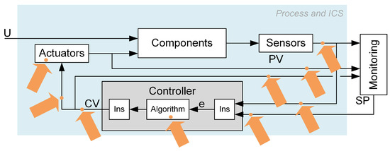
Figure 1.
Cyber-attack detection and isolation scheme based on controller modelling and loop performance indices.
Cyber-attacks entering the control system through the protection rings may destructively distort the measurement and control signals, the control algorithm, or its parameters. Potential attack vectors are illustrated in Figure 2. Each cyber-attack is carried out according to a designed scenario—a specific method of attack. Such a scenario consists of elementary impacts (partial actions) on individual system elements and signals in communication channels called cybernetic faults. “Cybernetic faults” plays an analogous role as “process faults” used by the FDI community. They represent a specific cause of the erroneous operation (or falsification of values) introduced by the attacker as a single step of the attack. The primary presented idea is to focus on the detection and isolation of cybernetic faults. However, the detection of any of the cybernetic faults equals the detection of a cyber-attack.
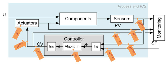
Figure 2.
Symbolic places of injection of attacks.
Therefore, real-time supervision of the control loops becomes necessary to detect intrusions into the control system early. The diagnostic system should detect and isolate both faults and attacks or its components.
This work aimed to develop and test algorithms to detect cyber-attacks and/or its components, i.e., cyber-faults, aimed at control algorithms. The paper shows that attack-detection methods based on controller models and control loop performance indicators are effective in this task. The attacks may, for example, modify the algorithm’s parameters. The change in the normal-reverse regulator operation mode leads to positive feedback. Changes in the settings may also result in the loss of system stability, and the modification of the setpoint value may result in the process entering the emergency area.
We also consider attacks directed at actuators, masking control values entering the process and or values entering the controller. We demonstrate effective detection in most cases and show further directions of research.
A case study was used as the research method. The possibilities of solving the formulated research problems were analysed on the example of a superheater system.
The proposed approach differs from the existing solutions in the following aspects:
- The approach is directed at the industrial controller.
- Only data from regular plant operations are needed.
- There are no specific requirements regarding the controlled process.
The structure of the paper is as follows: Section 2 presents the state-of-the-art in cyber-attack detection in control systems, Section 3.1 presents control loop performance indicators, and Section 3.2 introduces proposed controller modelling approaches. Preprocessing and merging of indicators are described in Section 3.3. Section 4 presents the case study, Section 5 the results, Section 6 shows a discussion of the results, and Section 7 concludes the paper.
2. Detection of Cyber-Attack on Control System
The protection of the control system against cyber-attacks is achieved primarily by using demilitarised zones, firewalls, data encryption, VPN (IPsec) networks, network segmentation, identity verification, access authorisation, and password management. Cyber-attack detection is carried out by monitoring network traffic that does not allow the detection of all anomalies [16]. The solutions used in IT systems do not guarantee the lack of possibility of an attack getting into the control system. Thus its destructive impact on the controlled process [17]. Early detection of anomalies and their isolation is essential to effectively respond to emerging hazards and threats.
The issues of cyber-attack detection in industrial control systems are developed very intensively [17,18,19,20,21]. Intrusion detection techniques against cyber-attacks are mainly divided into two categories: based on signatures and anomalies. Signature-based methods require a model of the system’s functioning in the case of a given type of attack. Anomaly-based attack detection techniques detect deviations from normal system behaviour. Similar approaches are used in fault diagnosis by the FDI community.
In terms of the detection of cyber-attacks in ICS, the following research directions can be distinguished: detection based on network traffic exploration, the analysis of network protocols, and the analysis of process data. ICS attacks often cause unusual network traffic or violate network protocol specifications. The methods of detecting these anomalies are derived from the methods used in IT systems. The above approaches are often used in Intrusion Detection Systems (IDS) [22]. Article [23] presents classifications of cyber attacks in network control systems and cyber-physical systems (CPS).
If the attacks penetrate the control system through the security measures applied, they affect the functioning of the control systems. Therefore, they can be detected as a discrepancy between the observed and reference activity, represented by models characterising the normal state of the controlled process. The detection scheme presented in [24,25] is identical to the fault detection scheme used for a long time in FDI methods.
There are passive and active approaches to detecting cyber-attacks. Passive methods are based on operating signals. Active methods require introducing an appropriate input signal and the analysis of its influence on the control systems. The active approach was presented in [26,27,28]. Observers [29,30], Kalman filters [31,32], and machine learning methods [33] were used as passive detection approaches. The use of neural models to detect anomalies was the subject of works [34,35]. Paper [36] investigates the attack isolation and attack location problems for a cyber-physical system based on the combination of the H-infinity observer and the zonotope theory. For anomaly detection, quantitative and qualitative models can be used. The works [2,37,38] present models in the form of rules that detect faults and attacks that cause the reverse controller operation or the actuator block. Developing benchmarks for testing and comparing cybersecurity solutions is also an active research area [39,40].
Research on cyber-attack detection tends to focus on a specific type of attack. The most significant amount of work is related to detecting false data injection attacks [34,41,42,43,44,45,46]. Fewer publications present studies of detection methods for replay attacks, covert attacks, and zero dynamics attacks [47].
Research on attack isolation is also emerging. The Anomaly Isolation Scheme (Iterative Observer Scheme) proposed in paper [48] is an extension of the well-known Generalised Observer Scheme, which was used to isolate single-sensor faults. The Unknown Input Observer is used to isolate cyber-attacks. In [49], a methodology based on the cyber-physical systems two side filters and an Unknown Input Observer-based detector has been proposed. A linear time-invariant (LTI) model was used, considering the impact of faults and cyber-attacks.
Our proposed approach does not require knowledge of process models with the impact of attacks and faults, nor does it assume a specific process form (such as LTI). All that is required is standard archived control loop data in the form of , , and signals and, for isolation, a binary diagnostic matrix, which is much simpler to obtain than the whole model.
Recently, attack detection based on control loop performance indices was proposed [50]. This method uses the Harris index, which, in its base version, was designed to fixe control systems. Additionally, the value of the Harris index is sensitive to the level of disturbances. Our goal is to propose a solution suitable for cascade control systems and includes isolation analysis. Therefore, we decide to rely on a larger number of simpler indices.
The detection methods derived from the approaches known in IT networks have already reached a high level of advancement, measured by many publications and the offered IDS systems using these techniques. The solutions derived from the approaches developed in the automation community, including intrusion detection based on process data analysis and control loop supervision, are more recent and less documented in publications. In the opinion of the authors of this paper, these methods that control the integrity of process data collected from measuring devices, actuators, and controllers may be of great practical importance. Methods developed based on fault diagnostics and models linking process variables can be used for this task.
The introduction of diagnostic systems that recognise both faults and cyber-attacks will constitute an additional layer of operational security (Layer of Protection) and another Ring of Protection in ICS.
3. Methods
3.1. Loop Performance Indicators
Many different indices of control quality are used in the literature and industrial software. Table 1 presents a list of indices, by category, that have been selected for initial testing. The indicators used in the final solution are indicated by . Indices in use are described in this section. For information regarding other indices, the reader is referred to the cited papers. During the preliminary tests, we found that the more complex indices (Harris index, oscillation factors) perform adequately, but their values are more challenging to interpret. In the application under consideration, we are mainly interested in the change in control quality and system behaviour. For this purpose, using more straightforward statistics for the control signal and control error is sufficient. These indicators are easy to interpret and calculate and do not require parameter selection. In addition, a set of dedicated indicators was also determined from the controller models.

Table 1.
Considered loop performance indicators ( points to the indicators selected for use in the final solution).
Indicators determined based on the response to a step change in were excluded due to the difficulty of application in the presence of significant disturbances and the inapplicability in fixed setpoint control systems or for auxiliary controllers in cascade control.
In the group of dedicated indicators, the estimation of the derivative time was omitted due to numerical difficulties when pre-filtering the signals fed to the controller.
The selected indices are calculated as follows (N—number of samples in a window):
- Mean absolute control error
- Mean squared control error
- Control signal variancewhere is the mean value of .
- Mean control signal difference between consecutive samples:
- Control signal oscillation (change in direction) count:where indicates the number of elements in x.
- Saturation index
3.2. Controller Modelling
The indices described in this section are not control loop performance measures. However, they have been proposed to detect changes in the controller algorithm that may result from malicious actions. A more detailed description and modelling results for different types of controllers can be found in [15].
In order to determine the indices for each control loop, two models are trained, estimating the increment in the control signal :
- The linear model is a linear regression model that takes the control error and lagged error values as inputs. The coefficients of the linear model allow the calculation of estimated PID controller settings. The model can only work for linear data—parts with regulator saturation are excluded from learning and prediction.
- The neural model is a non-linear model that takes control error and lagged error values and the control signal value as inputs. A model in the form of a multilayer perceptron was used. This model does not allow for controller settings estimation but can be used for controller types other than PID and data with controller saturation present.
Residuals of modelling errors are calculated as:
where is a linear model prediction and is a real controller output.
where is a neural model prediction.
Controller Settings Estimation Form Linear Model
This section presents only equations for the PI controller used in the case study. Details for other controller types can be found in [15].
The following equations were based on a linear model of the ideal PI controller in incremental version:
where k—sample number, , —control error, —proportional gain, and —integral time —sampling time.
The inputs of the controller model are and , and the model takes the form of:
where —model output, and and —model coefficients. The coefficients are estimated using mean squared error minimisation.
The controller parameters can be calculated using the estimated linear model coefficients:
3.3. Preprocessing
The signals considered are either a time series matched by sampling period to the controller processing period (e.g., ) or statistics or estimates determined for a specific time window (e.g., or ). In addition, each indicator has a different range of values, making it challenging to combine them and select alarm limits. Therefore, the following preprocessing steps were used (Figure 3):
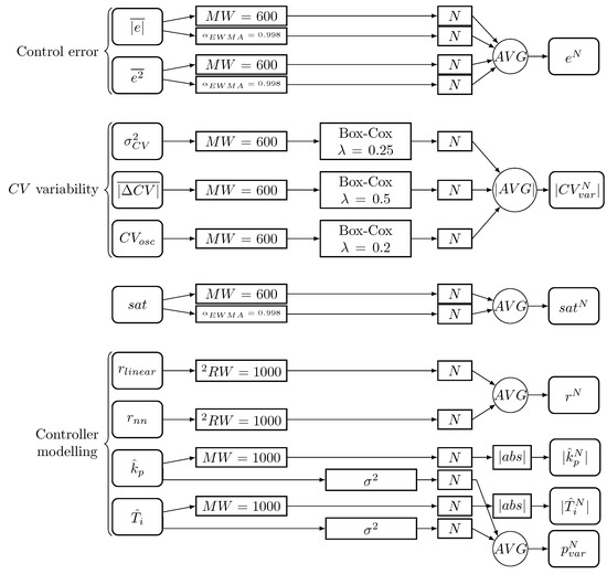
Figure 3.
Preprocessing.
- Control loop performance indices are calculated in mowing windows () and (if applicable) as exponentially weighted moving average ():
- -
- mowing windows are overlapping with an offset equal to half of the length of the moving window size
- -
- the exponentially weighted moving average of a time series is calculated as:where is the smoothing factor.
- The controller modelling residuals and are squared () and averaged in moving window with an offset equal to 1 ().
- The time series related to controller variability (, , ) has non-normal character. They are transformed using Box-Cox transformation:where is an exponent coefficient.
- All of the signals are normalised using a standard scaler (subtracting mean and dividing by standard deviation):where and denote the mean and standard deviation, respectively. Superscript denotes the normalised value.
- To achieve higher robustness and interpretability, the signals are grouped into indices according to the process feature that they describe:
- -
- Control error increase
- -
- Change in variability
- -
- High saturation
- -
- High controller model prediction error
- -
- Change in estimation
- -
- Change in estimation
- -
- High controller parameters estimation variability
After the preprocessing, we obtain the final set of signals:
These signals are thresholded to obtain the set of binarised alarm signals (diagnostic signals):
All of the preprocessing parameters (window sizes, smoothing factor , exponent for Box-Cox transformation, and alarm thresholds) are tuned using only the data from regular system operation (without any faults or cyber-faults). Controller models (linear and neural) are also fitted to the data from the regular operation. The current values of controller parameters’ estimates and are calculated from a linear model estimated in a sliding window. However, the model used for calculating residual is not updated.
3.4. Isolation Method
Our cyber-attack detection and isolation method is based on standard techniques used in the FDI community [4]. Fault detection and isolation are based on a set of diagnostic tests. Each j-th diagnostic test outputs a diagnostic signal indicating the result of the check. As a result of all the tests, we obtain the set of all diagnostic signals S:
To isolate the faults, it is necessary to know the relationship between the faults forming the set:
and the values of the diagnostic signals. Expert knowledge about the fault-symptom relation can be described and archived in many different forms. A binary relation can be represented by: logic functions, diagnostic trees, a binary diagnostic matrix, or a set of rules [4]. In the case under consideration, these faults will be cyber-attack scenarios.
The most popular method of fault-symptom relation representation is a binary diagnostic matrix (Table 2). It is defined over the Cartesian product of S and F, so it specifies the relation:
Table 2.
Binary matrix of relation.
The expression means that diagnostic signal is sensitive to fault . The occurrence of sets the value of to one, i.e., indicating a fault symptom. The matrix of this relation is called a binary diagnostic matrix (see the small example in Table 2). Each matrix entry is defined as follows:
Matrix element has a value of one if signal detects fault , and zero otherwise. A fault signature is a column vector containing the values of the diagnostic signals for this fault:
where .
Therefore, the columns of the binary diagnostic matrix (Table 2) correspond to fault signatures.
Given the binary diagnostic matrix and the actual values of diagnostic signals, we calculate the diagnosis by searching for the column of the binary diagnostic matrix with the maximal similarity to the values of diagnostic signals:
4. Case Study
The developed modelling approach was tested for a superheater system under malicious interventions. The study used a model of superheaters of the third and fourth stages of the steam line in the boiler of the power unit. The process schematic diagram with available measured process variables is given in Figure 4.
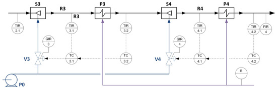
Figure 4.
A schematic process diagram with designated control loops and process variables.
The dynamic properties of the simulated process and its structure, including control loops and its parameters, were modelled based on the actual installation of a steam draught of the soda boiler in the paper company, which we collaborate with and which granted us access to process description, real data, and controller parameters, which were used during simulator elaboration. The simulator was implemented in the PExSim environment [54]. It is a computational and simulation environment developed at the Institute of Automatic Control and Robotics of the Warsaw University of Technology. It is visually similar to Simulink but is definitely simplified compared to it. It allows cyclic processing of signals according to the designed algorithm given in the form of a function block diagram. This is one of the possible simulation environments to be used. Choosing a specific simulation environment, i.e., its properties, do not have an impact on the conducted simulations and, consequently, on the results of the presented tests.
The modelled part of the process consists of the third and fourth steam line sections. In both, there are: attemperator, superheater, and cascade control systems—the main controller controls the temperature of the steam behind the superheater. The auxiliary controller controls the injection water valve and the temperature behind the cooler. The notation will be as follows: , —the auxiliary and main control loops of the third stage, respectively, , —the auxiliary and main control loops of the fourth stage, respectively. The available measurement variables directly related to the considered process with control loops, along with the determination of the ranges of variation and the operating points to which the model has been tuned based on data from the actual process, are characterised in Table 3.
Table 3.
Available process variables.
The process was modelled in a simulation environment using a simplified linearised (at an operating point) model, reflecting the fundamental relationships between physical quantities. A specific variability of input quantities was assumed in the conducted experiments (temperature and steam flow at the inlet to the third stage and the contractual value of the fuel flow fed to the boiler) and cycles of the variability of setpoint () values of the main controllers of the third and fourth stages: related changes in and .
According to the place of introduction (Figure 2), cybernetic faults have been divided into the following types (marked with a superficial upper index):
- — modification at the process output (visible to the operator and controller),
- — modification at the controller input (visible only by the controller),
- — modification at the controller input (invisible to the operator),
- —modification of the not-controlled process variable at the process output (visible to the operator and controller),
- —modification of at the controller output (visible to everyone),
- —modification of at the actuator input (visible only by the actuator),
- —modification of at the monitoring system input (visible to the operator),
- —modification (detailed described by x) of the controller’s operation,
- —modification (detailed described by x) of the operation of the actuator.
The lower index indicates the control loop or specific component affected by the attack. In order to test different cyber-attack scenarios, the simulator includes the possibility of simulating cybernetic faults presented in Notations. The symbolic place of introducing the cybernetic faults performed during selected cyber-attacks is shown in Figure 5.
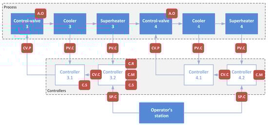
Figure 5.
Places of influence on the process during the implementation of cyber-attacks (by the type of cybernetic fault).
The number of possible attack scenarios is practically unlimited. The use of different scenarios was considered in terms of the conducted research. They were divided into groups depending on the attack component or group of signals. The particular groups can be characterised as follows:
- attack on the controller (change in operating mode, change in parameters),
- modification in set points,
- modification in control variables,
- modification in controlled variables,
- attack on the actuator (blockage, modification in operation, changes in operating parameters).
Originally, we evaluated 27 cyber-attack scenarios of 12 types with different detailed parameters. However, we have decided to discuss, in this paper, only a subset of scenarios strictly related to controllers and most interesting to investigate. The particular cyber-attack scenarios selected for detailed research are presented in Table 4.
Table 4.
The set of cyber-attack scenarios (CAS). Each attack starts at (s).
A specific variability of input signals, B, , and , symbolising disturbance, was assumed to generate learning and testing data. The value of each signal is the sum of four sinusoidal signals (with different parameters) and two random signals (with normal distribution but different gains), which are additionally processed by an inertial element to eliminate violent, physically unrealisable changes. The variability of individual signals is turned on or off at specified intervals every 6 h. Work scenarios for (a) constant values and (b) variable values according to a given scenario were also considered.
The dataset containing signals for all the considered scenarios and normal process operation is available at https://doi.org/10.5281/zenodo.7612269.
Binary Diagnostic Matrix for Considered Scenarios
Based on the knowledge of the nature of the scenarios, an initial version of the binary diagnostic matrix presented in Table 5 was developed. It can be observed that some of the columns of the diagnostic matrix are the same, which means that the proposed diagnostic signals cannot isolate the given scenarios. Thus, to simplify, a reduced version of the binary diagnostic matrix was prepared, where the indistinguishable scenarios were combined. The reduced binary diagnostic matrix is presented in Table 6.
Table 5.
Initial binary diagnostic matrix.
Table 6.
Reduced binary diagnostic matrix.
The linear model (and thus the controller parameter estimation) only works if the controller is not saturated, hence the blanks in the table for the CON-1 scenario.
The columns of the reduced binary diagnostic matrix (Table 6) can be interpreted as follows: cyber-attack CON-12 denotes an attack directed at the controller of a drastic nature (switching to manual mode, changing from normal to reverse). In this case, we observe a residuum of the controller model () as well as a deterioration in the quality of system operation (high control error).
The CON-3 scenario denotes changes in the controller (e.g., a change in the settings) but of a nature that does not entirely prevent the system’s operation. We observe an error in the controller model and changes in the settings estimation, but the control quality does not deteriorate drastically. In the case of a PID controller, more accurate information about changes can be obtained from the values of the estimated settings.
PVSP scenarios imply falsification of the values fed to the controller ( or , respectively). In this case, we receive alarms about the regulator’s model error and the change in the settings estimate. However, in contrast to the CON-3 scenario, the settings estimates are inconsistent and have a high variance. The control error increases, but we do not observe a change in the character of the controller output (saturation or variance change) because the controller is operating correctly but on different values, than are recorded by the operator.
ACTCV scenarios represent attacks directed at the actuator or falsification of the value fed to the process, respectively. From the point of view of the controller models and control quality indicators, this is visible as a process change. The controller works correctly (the models show no deviation), but the regulation quality deteriorates (the control error increases), and the controller can enter a saturation zone. Note that changes in the process or actuator that the controller can compensate for will not be detectable, as will be demonstrated in the example scenario .
5. Results
This section will discuss the results obtained for the test scenarios.
Table 7 shows the results obtained without cyber-attacks. The attack starts in the middle of a given data file in each scenario. The data before the attacks were used to evaluate the performance in the normal state. Table 7 shows the results averaged over all scenarios. The columns show the subsequent control circuits. The rows show the averaged values of the alarm signals. The row indicates the percentage of correct diagnoses (in this case, the correct diagnosis is always normal). The row presents the false positive alarm rate, which equals . We can see that the percentage of false alarms is low for individual diagnostic signals and resultant diagnoses, and the system works correctly in cases without cyber-attacks.
Table 7.
The values of diagnostic signals during normal operation (each column shows one control loop).
The actual ( and ) and estimated ( and ) values of the controller settings are shown in Table 8. The columns show the subsequent scenarios. Note that some of the scenarios involve changing the settings. The estimates of the settings are close to the actual values and provide valuable diagnostic information in the case of attacks. The errors of the estimates are significant only for scenarios and , where spurious signal values are fed into the controller. We can detect this situation based on the variance in the parameter estimate .
Table 8.
Settings estimation.
The performance results during the attacks are presented by the control loop in Table 9, Table 10, Table 11 and Table 12. The columns show the subsequent scenarios. Note that each attack can affect from one to all control loops. The names of the scenarios in which a particular loop is affected have been bolded. When an attack does not affect a loop, the correct diagnosis is normal. The rows show the average values of the diagnostic signals during the attack. denotes the percentage of correct diagnoses, denotes the percentage of attack detections (diagnoses other than normal), and is the most frequent diagnosis. The tables are divided by a vertical line into a controller-directed attack part (left part) and a process-directed attack part (right part). The left-hand part demonstrates the proposed approach’s effectiveness in detecting and localising controller cyber-attacks. The right-hand section presents tests for process-directed attacks. The purpose of this part is to test the applicability and deficits of the proposed approach and to provide directions for further work.
Table 9.
The values of diagnostic signals in loop during attacks. Bolded column names indicate scenarios affecting this loop.
Table 10.
The values of diagnostic signals in loop 3.2 during attacks. Bolded column names indicate scenarios affecting this loop.
Table 11.
The values of diagnostic signals in loop 4.1 during attacks. Bolded column names indicate scenarios affecting this loop.
Table 12.
The values of diagnostic signals in loop 4.2 during attacks. Bolded column names indicate scenarios affecting this loop.
For the scenarios considered, the fault isolation process involves two issues. One is to decide which control circuit is affected by the attack and what attack it is. It should be noted that an attack on one of the control circuits can change the operating conditions of the entire process, so it significantly increases the risk of false alarms in the other loops. However, it is most important to identify the loop that needs to be addressed first.
The results of the cyber-attack isolation are shown in Table 13 and Table 14. Table 15 indicates which attacks affect which loop. This provides a template for the correct locations regarding control loop selection. Table 13 shows the results obtained regarding control loop isolation. A value of 1 indicates that the diagnosis differed from the normal state in the respective loop over 50% of the time. Incorrect values are marked in red. We can observe that scenario was not detected in any control loop—the case of this scenario will be analysed in detail in the plots. All other scenarios were detected. For the controller scenarios, the isolation in terms of the control circuit is precise (one false alarm for loop 4.1). False alarms for the scenarios and appear on the left-hand side of the table. These are due to the significant impact of the deterioration in the main circuit on the auxiliary circuit () and the impact of the deterioration in stage 3 on the operation of stage 4 ().
Table 13.
Attack detection results for each loop. Red color indicates incorrect values.
Table 14.
Most common diagnosis for each loop and each scenario. Red color indicates incorrect values.
Table 15.
Affected loops in each scenario.
The results of the isolation in terms of the scenario are shown in Table 14. Again, attacks targeting the controller operation were correctly identified (one false alarm for loop 4.1). Scenario involves substituting the value of for a fixed value and can only be correctly detected and recognised when the actual value of differs from the provided fixed value. This is explained in more detail in the graphs in (Figure 6 and Figure 7). The two attacked loops indicate the correct diagnosis for scenario . Scenario was correctly detected but is mistaken for a CON-12 diagnosis.
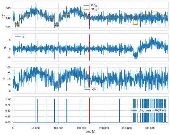
Figure 6.
Scenario , loop , values of , , e, and . The lowest plot shows the presence of the correct diagnosis . Red vertical line indicates the beginning of cyber-attack.
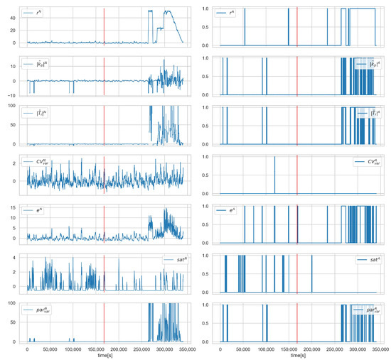
Figure 7.
Scenario , loop , values of normalised signals (left), and binarised diagnostic signals (right). Red vertical line indicates the beginning of cyber-attack.
Figure 8, Figure 9 and Figure 10 show the runs for scenario and control loop 3.1. This scenario involves changing the controller settings to less aggressive. Figure 8 shows , , e, and , respectively. The red vertical line indicates the moment of attack. Figure 9 shows the estimated and actual parameter values. We can see that the estimates are close to the actual values. The values of the diagnostic signals are shown in Figure 10. These signals behave as predicted—we observe alarms for the model error and the controller parameter estimates. Intermittent alarms indicate an increase in the control deviation, which is consistent with the actual state.
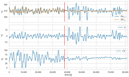
Figure 8.
Scenario , loop , values of , , e, and . Red vertical line indicates the beginning of cyber-attack.
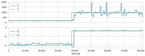
Figure 9.
Scenario , loop , and controller settings estimates (blue—estimates, green—actual values).
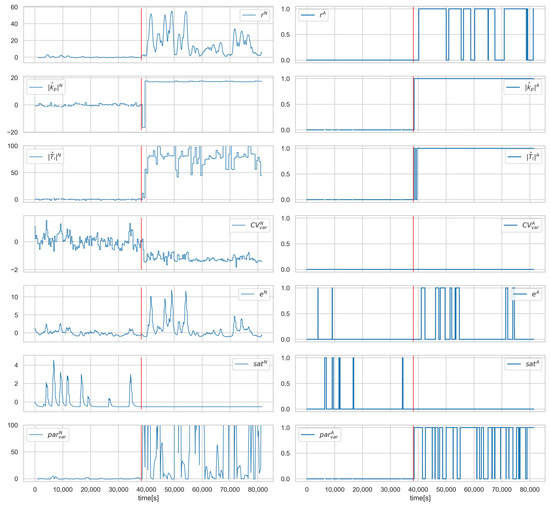
Figure 10.
Scenario , loop , values of normalised signals (left), and binarised diagnostic signals (right). Red vertical line indicates the beginning of cyber-attack.
Figure 6 and Figure 7 show the runs for scenario and control loop 4.2. Figure 6 shows the values of the variables and, in the lower plot, the presence of the correct diagnosis . This scenario consists of substituting the value fed to the controller. Symptoms of this attack can only be observed when the actual value deviates from the falsified one, which is observed from about 260,000 s. The same dependence can be observed for the diagnostic signals (Figure 7).
Figure 11 and Figure 12 show the values of the process and alarm signals, respectively, for scenario and loop 3.1. In this scenario, the control valve is attacked (its closure ratio is changed by 20 %). We can observe, in Figure 11, that this causes a change in the average value of . However, the control system can compensate for the attack, and we do not observe a deterioration in the quality of the control. This can also be seen in the diagnostic signals (Figure 12)—only a slight increase in the saturation index is visible. Since the controller is working correctly and there is no evident deterioration of the control quality, this scenario is impossible to detect in the proposed solution. In the authors’ opinion, this problem should be solved by introducing process models into the system in further development.
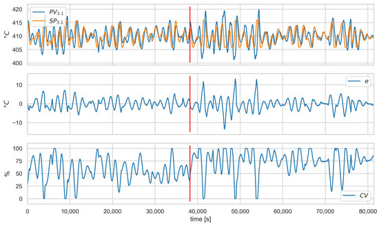
Figure 11.
Scenario , loop , values of , , e, and . Red vertical line indicates the beginning of cyber-attack.
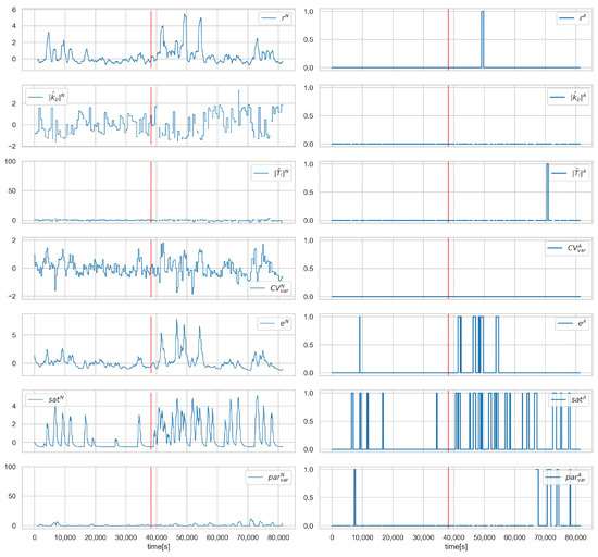
Figure 12.
Scenario , loop , values of normalised signals (left), and binarised diagnostic signals (right). Red vertical line indicates the beginning of cyber-attack.
Sensitivity Analysis
As part of the sensitivity analysis, the robustness of the proposed method to process changes and changes in the nature of cyber-faults was tested. For this purpose, a baseline scenario containing two cyber-faults, and , involving a change in controller settings to a more aggressive one was modified. Modifications of , , and of the baseline change were applied. The specific values of the controller settings are given in Table 16. The effect of varying the amplitude of the disturbance was also tested. The disturbance was taking and of the baseline value ( and scenarios, respectively).
Table 16.
Settings estimation for scenario under different disturbances and cyber-fault sizes.
No modifications were made to the method or parameters. The same neural networks and linear models were used in the tests as in the earlier experiments. The models were trained with a baseline level of noise. The data normalisation factors and alarm thresholds were not changed.
The results are presented in Table 17. For each scenario, the percentage of detection, , and percentage of correct diagnoses, , are shown. The results are shown for each loop. In this scenario, loops and are attacked, and these column names have been bolded. We can see that the isolation within the control loop continues to be very precise. Missed detections can be observed for small settings changes (). For significant disturbances, few false alarms appear for the and loops. For substantial settings changes (), the cyber-attack type isolation starts to indicate the scenario. This scenario means drastic changes in the controller preventing effective regulation, and this classification for significant settings changes can be considered correct.
Table 17.
Detection and isolation for scenario under different disturbances and cyber-fault sizes.
The results of estimating the controller settings under different conditions are shown in Table 16. The settings are estimated correctly with an accuracy close to the baseline scenarios.
From the tests, it can be concluded that the proposed method has some robustness. Of course, detecting small changes in the presence of significant disturbances will be difficult. Further, a change in the system’s operating conditions (change in the nature of the inputs, severity of the disturbances) may lead to the need for retraining the models and re-tuning the normalisation factors and alarm limits. Both of these processes can be carried out automatically once new, representative data have been acquired.
6. Discussion
This work presents controller modelling and control loop performance indicators as tools for detecting and isolating cyber-attacks. Controller models allow the detection of changes in controller performance and settings (in the case of PID controllers). Control quality indicators allow an overall assessment of the performance of control circuits and the detection of deterioration in control quality.
The selection of suitable control quality indices and the preprocessing and combining of signals to obtain a set of interpretable indices are presented.
The operation of the concept was tested on a superheater system. The system’s overall performance should be considered a valuable indication for the process operator. In regular operation, the percentage of false alarms is low at . All attacks except were detected (the issue of not being able to detect attack is further detailed in Figure 11 and Figure 12).
The system performs very well in attacks directly targeting the controller’s operation. All attacks were correctly detected. The detection percentage in the attacked loops is (attacks relating to a given loop are indicated in bold in Table 9, Table 10, Table 11 and Table 12). The isolation of the control loop is accurate (one false alarm for loop in scenario ). The isolation in terms of scenarios is also accurate (the same false alarm for loop 4.1 in scenario ), and interpretable diagnostic signals allow the nature of the attack (such as the nature of the setting change) to be identified more accurately. The system’s overall accuracy (percentage of correct diagnoses) is .
In terms of other attacks, the system provides valuable indications of system changes—all attacks except have been detected. The attacked circuits are mainly indicated as the source of the problem ( percentage of detection for an attack except for ). However, the change in operating conditions also increases the occurrence of alarms in the remaining control loops, even if they are not directly affected by the attack. Scenario shows that process models are needed to detect attacks that the controller action can mask.
It should be noted that indicators calculated in a sliding window (such as PID controller parameter estimates) inevitably introduce fault detection and isolation delays. Using process models is a way to obtain indicators that react faster to anomalies.
7. Conclusions
In advanced diagnostics of industrial control systems (ICS) performed automatically, faults and cyber-attacks should be detected and isolated. Compared to the classic FDI approach, the area of diagnostic activities is, therefore, extended and should include not only process apparatus, measurements, and actuators but also units implementing control algorithms. Controller models and control loop performance indicators can be used effectively to detect cyber-attacks and faults that manifest in changes to control systems’ operation. The isolation of controller faults and cyber-attacks can be performed using inference methods based on the binary diagnostic matrix. The case study showed that correct identification of malfunctioning control loops and introduced cyber-attack scenarios could be achieved. Experimental verification should be carried out on a process simulator allowing the introduction of both faults and cyber-attacks.
It is planned to test additional scenarios in this way. The conduct of industrial tests is much more problematic due to limitations on the possibility of introducing faults and cyber-attacks. In addition, consent for such experiments will not be given by company management due to the risks of such research. In this situation, industrial verification can take place after thorough simulation verification during a pilot implementation on a real installation.
The direction of further work is to develop an integrated approach for fault and cyber-attack detection and isolation in ICS, which should additionally include detection based on process and actuator models and the isolation of cyber-attacks and faults based not only on binary residual evaluation but also on trivalent evaluation.
Author Contributions
Conceptualisation, A.S.-B. and J.M.K.; Data curation, A.S.-B. and M.S.; Formal analysis, A.S.-B. and J.M.K.; Funding acquisition, M.S.; Investigation, A.S.-B. and J.M.K.; Methodology, A.S.-B., J.M.K. and Z.G.; Project administration, M.S.; Resources, M.S.; Software, A.S.-B., M.S. and Z.G.; Supervision, A.S.-B.; Validation, A.S.-B., M.S. and J.M.K.; Visualisation, A.S.-B. and M.S.; Writing—original draft, A.S.-B., M.S., J.M.K. and Z.G.; Writing—review and editing, A.S.-B. All authors have read and agreed to the published version of the manuscript.
Funding
This research was funded by European Funds grant number POIR.01.01.01-00-0541/20.
Institutional Review Board Statement
Not applicable.
Informed Consent Statement
Not applicable.
Data Availability Statement
Data are available at https://doi.org/10.5281/zenodo.7612269.
Conflicts of Interest
The authors declare no conflict of interest.
Abbreviations
The following abbreviations are used in this manuscript:
| Process Variable | |
| Set Point | |
| Control Signal | |
| ICS | Industrial Control Systems |
| IDS | Intrusion Detection Systems |
| CPS | Cyber-Physical Systems |
| FDI | Fault Detection and Isolation |
| IAE | Integral Absolute Error |
| MW | Moving Window |
| EWMA | Exponentially Weighted Moving Average |
| RW | Rolling Window |
Notations
List of simulated cybernetic faults.
| , | Changing the operating mode (to “manual”) of the indicated control loop |
| , | Modification (type C) of the control value of the indicated loop |
| , | Changing the operating mode (to “reverse”) of the indicated control loop |
| , | Changing the settings (, ) of the indicated control loop |
| , | Modification (type C) of the setpoint SP of the indicated loop |
| , | Modification (type P) of the control value of the indicated loop |
| , , , | Modification (type C) of the process value of the indicated loop |
| , , , | Modification (type P) of the process value of the indicated loop |
| , | Taking control of the operation of the indicated actuator |
| Changing the operating parameters (dead band) of the indicated actuator |
References
- Genge, B.; Kiss, I.; Haller, P. A System Dynamics Approach for Assessing the Impact of Cyber Attacks on Critical Infrastructures. Int. J. Crit. Infrastruct. Prot. 2015, 10, 3–17. [Google Scholar] [CrossRef]
- Kościelny, J.; Syfert, M.; Ordys, A.; Wnuk, P.; Możaryn, J.; Fajdek, B.; Puig, V.; Kukiełka, K. Towards a unified approach to detection of faults and cyber-attacks in industrial installations. In Proceedings of the European Control Conference, Delft, The Netherlands, 29 June–2 July 2021; pp. 1839–1844. [Google Scholar]
- Rubio, J.E.; Román, R.; López, J. Analysis of Cybersecurity Threats in Industry 4.0: The Case of Intrusion Detection. In Proceedings of the CRITIS, Lucca, Italy, 8–13 October 2017. [Google Scholar]
- Korbicz, J.; Kowalczuk, Z.; Kościelny, J.M.; Cholewa, W. (Eds.) Fault Diagnosis: Models, Artificial Intelligence Methods, Applications; Springer: Berlin/Heidelberg, Germany, 1998. [Google Scholar]
- Gertler, J. Fault Detection and Diagnosis in Engineering Systems; Marcel Dekker, Inc.: New York, NY, USA, 1998. [Google Scholar]
- Zhong, M.; Xue, T.; Ding, S.X. A survey on model-based fault diagnosis for linear discrete time-varying systems. Neurocomputing 2018, 306, 51–60. [Google Scholar] [CrossRef]
- Li, D.; Wang, Y.; Wang, J.; Wang, C.; Duan, Y. Recent advances in sensor fault diagnosis: A review. Sens. Actuators A Phys. 2020, 309, 111990. [Google Scholar] [CrossRef]
- Park, Y.J.; Fan, S.K.S.; Hsu, C.Y. A Review on Fault Detection and Process Diagnostics in Industrial Processes. Processes 2020, 8, 1123. [Google Scholar] [CrossRef]
- Ju, Y.; Tian, X.; Liu, H.; Ma, L. Fault detection of networked dynamical systems: A survey of trends and techniques. Int. J. Syst. Sci. 2021, 52, 3390–3409. [Google Scholar] [CrossRef]
- Bauer, M.; Horch, A.; Xie, L.; Jelali, M.; Thornhill, N. The current state of control loop performance monitoring—A survey of application in industry. J. Process Control 2016, 38, 1–10. [Google Scholar] [CrossRef]
- Harris, T.J. Assessment of control loop performance. Can. J. Chem. Eng. 1989, 67, 856–861. [Google Scholar] [CrossRef]
- Starr, K.D.; Petersen, H.; Bauer, M. Control loop performance monitoring—ABB’s experience over two decades. IFAC-PapersOnLine 2016, 49, 526–532. [Google Scholar] [CrossRef]
- Ordys, A.; Uduehi, D.; Johnson, M.A. Process Control Performance Assessment: From Theory to Implementation; Springer: London, UK, 2007. [Google Scholar]
- Jelali, M. Control Performance Management in Industrial Automation: Assessment, Diagnosis and Improvement of Control Loop Performance; Springer: London, UK, 2013. [Google Scholar]
- Sztyber, A.; Górecka, Z.; Kościelny, J.M.; Syfert, M. Controller Modelling as a Tool for Cyber-Attacks Detection. In Proceedings of the International Conference on Diagnostics of Processes and Systems DPS 2022, Chmielno, Poland, 5–7 September 2022; Intelligent and Safe Computer Systems in Control and Diagnostics. Kowalczuk, Z., Ed.; Springer International Publishing: Cham, Switzerland, 2023; pp. 100–111. [Google Scholar]
- Cardenas, A.; Amin, S.; Sinopoli, B.; Giani, A.; Perrig, A.; Sastry, S. Challenges for Securing Cyber Physical Systems. In Proceedings of the Workshop on Future Directions in Cyber-Physical Systems Security, Newark, NJ, USA, 22–24 July 2009. [Google Scholar]
- Ding, D.; Han, Q.L.; Xiang, Y.; Ge, X.; Zhang, X.M. A Survey on Security Control and Attack Detection for Industrial Cyber-Physical Systems. Neurocomputing 2018, 275, 1674–1683. [Google Scholar] [CrossRef]
- Jang-Jaccard, J.; Nepal, S. A survey of emerging threats in cybersecurity. J. Comput. Syst. Sci. 2014, 80, 973–993. [Google Scholar] [CrossRef]
- Sánchez, H.S.; Rotondo, D.; Escobet, T.; Puig, V.; Quevedo, J. Bibliographical review on cyber attacks from a control oriented perspective. Annu. Rev. Control 2019, 48, 103–128. [Google Scholar] [CrossRef]
- Mahmoud, M.S.; Hamdan, M.M.; Baroudi, U.A. Modeling and control of Cyber-Physical Systems subject to cyber attacks: A survey of recent advances and challenges. Neurocomputing 2019, 338, 101–115. [Google Scholar] [CrossRef]
- Loukas, G. 4—Cyber-Physical Attacks on Industrial Control Systems. In Cyber-Physical Attacks; Loukas, G., Ed.; Butterworth-Heinemann: Boston, MA, USA, 2015; pp. 105–144. [Google Scholar] [CrossRef]
- Mitchell, R.; Chen, I.R. A Survey of Intrusion Detection Techniques for Cyber-Physical Systems. ACM Comput. Surv. 2014, 46, 1–29. [Google Scholar] [CrossRef]
- Teixeira, A.; Shames, I.; Sandberg, H.; Johansson, K.H. A secure control framework for resource-limited adversaries. Automatica 2015, 51, 135–148. [Google Scholar] [CrossRef]
- Hu, Y.; Li, H.; Yang, H.; Sun, Y.; Sun, L.; Wang, Z. Detecting stealthy attacks against industrial control systems based on residual skewness analysis. EURASIP J. Wirel. Commun. Netw. 2019, 74. [Google Scholar] [CrossRef]
- Urbina, D.I.; Giraldo, J.A.; Cardenas, A.A.; Tippenhauer, N.O.; Valente, J.; Faisal, M.; Ruths, J.; Candell, R.; Sandberg, H. Limiting the Impact of Stealthy Attacks on Industrial Control Systems. In Proceedings of the 2016 ACM SIGSAC Conference on Computer and Communications Security, Vienna, Austria, 24–28 October 2016; pp. 1092–1105. [Google Scholar]
- Trapiello, C.; Rotondo, D.; Sanchez, H.; Puig, V. Detection of replay attacks in CPSs using observer-based signature compensation. In Proceedings of the 2019 6th International Conference on Control, Decision and Information Technologies (CoDIT), Paris, France, 23–26 April 2019; pp. 1–6. [Google Scholar] [CrossRef]
- Trapiello, C.; Puig, V. Replay attack detection using a zonotopic KF and LQ approach. In Proceedings of the 2020 IEEE International Conference on Systems, Man, and Cybernetics (SMC), Toronto, ON, Canada, 11–14 October 2020; pp. 3117–3122. [Google Scholar]
- Trapiello, C.; Puig, V. Input Design for Active Dectection of Integrity Attacks using Set-based Approach. IFAC-PapersOnLine 2020, 53, 11094–11099. [Google Scholar] [CrossRef]
- Pasqualetti, F.; Dörfler, F.; Bullo, F. Attack Detection and Identification in Cyber-Physical Systems. IEEE Trans. Autom. Control 2013, 58, 2715–2729. [Google Scholar] [CrossRef]
- Ao, W.; Song, Y.; Wen, C. Adaptive cyber-physical system attack detection and reconstruction with application to power systems. IET Control Theory Appl. 2016, 10, 1458–1468. [Google Scholar] [CrossRef]
- Sinopoli, B.; Schenato, L.; Franceschetti, M.; Poolla, K.; Jordan, M.; Sastry, S. Kalman filtering with intermittent observations. IEEE Trans. Autom. Control 2004, 49, 1453–1464. [Google Scholar] [CrossRef]
- Cong, T.; Tan, R.; Ottewill, J.R.; Thornhill, N.F.; Baranowski, J. Anomaly Detection and Mode Identification in Multimode Processes Using the Field Kalman Filter. IEEE Trans. Control Syst. Technol. 2021, 29, 2192–2205. [Google Scholar] [CrossRef]
- Bedi, P.; Mewada, S.; Vatti, R.A.; Singh, C.; Dhindsa, K.S.; Ponnusamy, M.; Sikarwar, R. Detection of attacks in IoT sensors networks using machine learning algorithm. Microprocess. Microsyst. 2021, 82, 103814. [Google Scholar] [CrossRef]
- Abbaspour, A.; Sargolzaei, A.; Yen, K. Detection of false data injection attack on load frequency control in distributed power systems. In Proceedings of the 2017 North American Power Symposium (NAPS), Morgantown, WV, USA, 17–19 September 2017; pp. 1–6. [Google Scholar]
- Wu, Z.; Albalawi, F.; Zhang, J.; Zhang, Z.; Durand, H.; Christofides, P.D. Detecting and Handling Cyber-Attacks in Model Predictive Control of Chemical Processes. Mathematics 2018, 6, 173. [Google Scholar] [CrossRef]
- Zhang, X.; Zhu, F.; Zhang, J.; Liu, T. Attack isolation and location for a complex network cyber-physical system via zonotope theory. Neurocomputing 2022, 469, 239–250. [Google Scholar] [CrossRef]
- Kościelny, J.; Syfert, M.; Wnuk, P. The Idea of On-line Diagnostics as a Method of Cyberattack. In Advanced Solutions in Diagnostics and Fault Tolerant Control; Kościelny, J.M., Syfert, M., Sztyber, A., Eds.; Springer: Cham, Switzerland, 2018; pp. 449–457. [Google Scholar]
- Syfert, M.; Ordys, A.; Kościelny, J.M.; Wnuk, P.; Możaryn, J.; Kukiełka, K. Integrated Approach to Diagnostics of Failures and Cyber-Attacks in Industrial Control Systems. Energies 2022, 15, 6212. [Google Scholar] [CrossRef]
- Syfert, M.; Kościelny, J.M.; Możaryn, J.; Ordys, A.; Wnuk, P. Simulation Model and Scenarios for Testing Detectability of Cyberattacks in Industrial Control Systems. In Proceedings of the International Conference on Diagnostics of Processes and Systems DPS 2022, Chmielno, Poland, 5–7 September 2022; Intelligent and Safe Computer Systems in Control and Diagnostics. Kowalczuk, Z., Ed.; Springer International Publishing: Cham, Switzerland, 2023; pp. 73–84. [Google Scholar]
- Quevedo, J.; Sánchez, H.; Rotondo, D.; Escobet, T.; Puig, V. A two-tank benchmark for detection and isolation of cyber attacks. IFAC-PapersOnLine 2018, 51, 770–775. [Google Scholar] [CrossRef]
- Bobba, R.B.; Rogers, K.M.; Wang, Q.; Khurana, H.; Nahrstedt, K.; Overbye, T.J. Detecting false data injection attacks on dc state estimation. In Preprints of the First Workshop on Secure Control Systems; CPSWEEK: Stockholm, Sweden, 2010; Volume 2010. [Google Scholar]
- Yang, Q.; Yang, J.; Yu, W.; An, D.; Zhang, N.; Zhao, W. On False Data-Injection Attacks against Power System State Estimation: Modeling and Countermeasures. IEEE Trans. Parallel Distrib. Syst. 2014, 25, 717–729. [Google Scholar] [CrossRef]
- Chaojun, G.; Jirutitijaroen, P.; Motani, M. Detecting False Data Injection Attacks in AC State Estimation. IEEE Trans. Smart Grid 2015, 6, 2476–2483. [Google Scholar] [CrossRef]
- Huang, Y.; Li, H.; Campbell, K.A.; Han, Z. Defending false data injection attack on smart grid network using adaptive CUSUM test. In Proceedings of the 2011 45th Annual Conference on Information Sciences and Systems, Baltimore, MD, USA, 23–25 March 2011; pp. 1–6. [Google Scholar] [CrossRef]
- Kontouras, E.; Tzes, A.; Dritsas, L. Impact Analysis of a Bias Injection Cyber-Attack on a Power Plant. IFAC-PapersOnLine 2017, 50, 11094–11099. [Google Scholar] [CrossRef]
- Wang, X.; Luo, X.; Zhang, Y.; Guan, X. Detection and Isolation of False Data Injection Attacks in Smart Grids via Nonlinear Interval Observer. IEEE Internet Things J. 2019, 6, 6498–6512. [Google Scholar] [CrossRef]
- Hoehn, A.; Zhang, P. Detection of replay attacks in cyber-physical systems. In Proceedings of the 2016 American Control Conference (ACC), Boston, MA, USA, 6–8 July 2016; pp. 290–295. [Google Scholar] [CrossRef]
- Manandhar, K.; Cao, X. Attacks/faults detection and isolation in the Smart Grid using Kalman Filter. In Proceedings of the 2014 23rd International Conference on Computer Communication and Networks (ICCCN), Shanghai, China, 4–7 August 2014; pp. 1–6. [Google Scholar] [CrossRef]
- Taheri, M.; Khorasani, K.; Shames, I.; Meskin, N. Cyber Attack and Machine Induced Fault Detection and Isolation Methodologies for Cyber-Physical Systems. arXiv 2020, arXiv:2009.06196. [Google Scholar]
- Możaryn, J.F.; Frątczak, M.; Stebel, K.; Kłopot, T.; Nocoń, W.; Ordys, A.; Ozana, S. Stealthy Cyberattacks Detection Based on Control Performance Assessment Methods for the Air Conditioning Industrial Installation. Energies 2023, 16, 1290. [Google Scholar] [CrossRef]
- Swanda, A.; Seborg, D. Controller performance assessment based on setpoint response data. In Proceedings of the 1999 American Control Conference (Cat. No. 99CH36251), San Diego, CA, USA, 2–4 June 1999; Volume 6, pp. 3863–3867. [Google Scholar] [CrossRef]
- Hägglund, T. A control-loop performance monitor. Control Eng. Pract. 1995, 3, 1543–1551. [Google Scholar] [CrossRef]
- Thornhill, N.; Huang, B.; Zhang, H. Detection of multiple oscillations in control loops. J. Process Control 2003, 13, 91–100. [Google Scholar] [CrossRef]
- Syfert, M.; Wnuk, P. Signal Processing in DiaSter System for Simulation and Diagnostic Purposes. In Proceedings of the 10th International Conference Mechatronics 2013, Brno, Czech Republic, 7–9 October 2013; Mechatronics 2013. Březina, T., Jabloński, R., Eds.; Springer International Publishing: Cham, Switzerland, 2014; pp. 441–448. [Google Scholar]
Disclaimer/Publisher’s Note: The statements, opinions and data contained in all publications are solely those of the individual author(s) and contributor(s) and not of MDPI and/or the editor(s). MDPI and/or the editor(s) disclaim responsibility for any injury to people or property resulting from any ideas, methods, instructions or products referred to in the content. |
© 2023 by the authors. Licensee MDPI, Basel, Switzerland. This article is an open access article distributed under the terms and conditions of the Creative Commons Attribution (CC BY) license (https://creativecommons.org/licenses/by/4.0/).