
Massive MIMO Indoor Transmissions at 38 and 65 GHz Applying Novel HBF Techniques for 5G

 , and
, and
Abstract
:1. Introduction
2. Description of the Experimental Setup
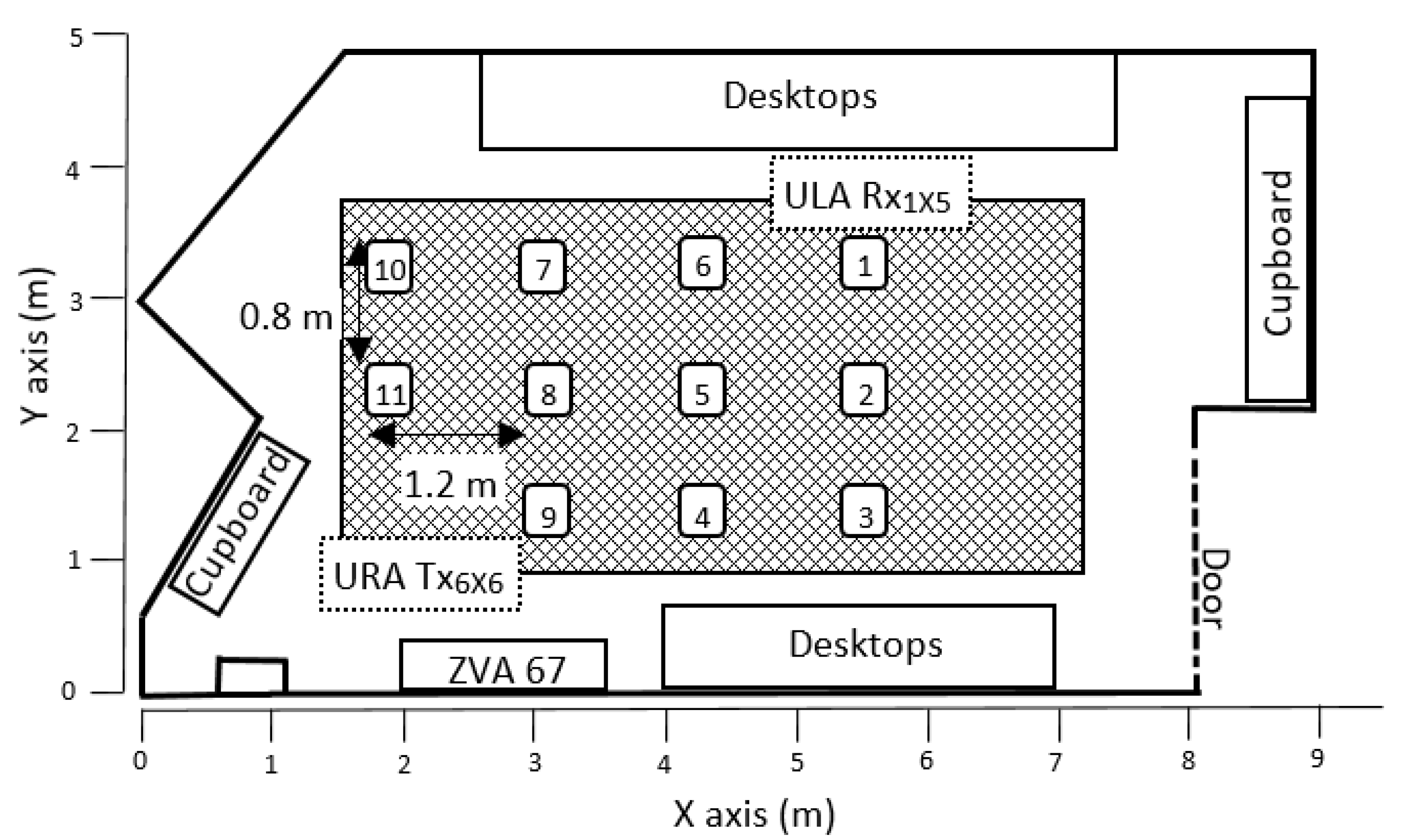
2.1. Scenario
2.2. Channel Sounder
3. Methodology
3.1. Implemented Algorithms
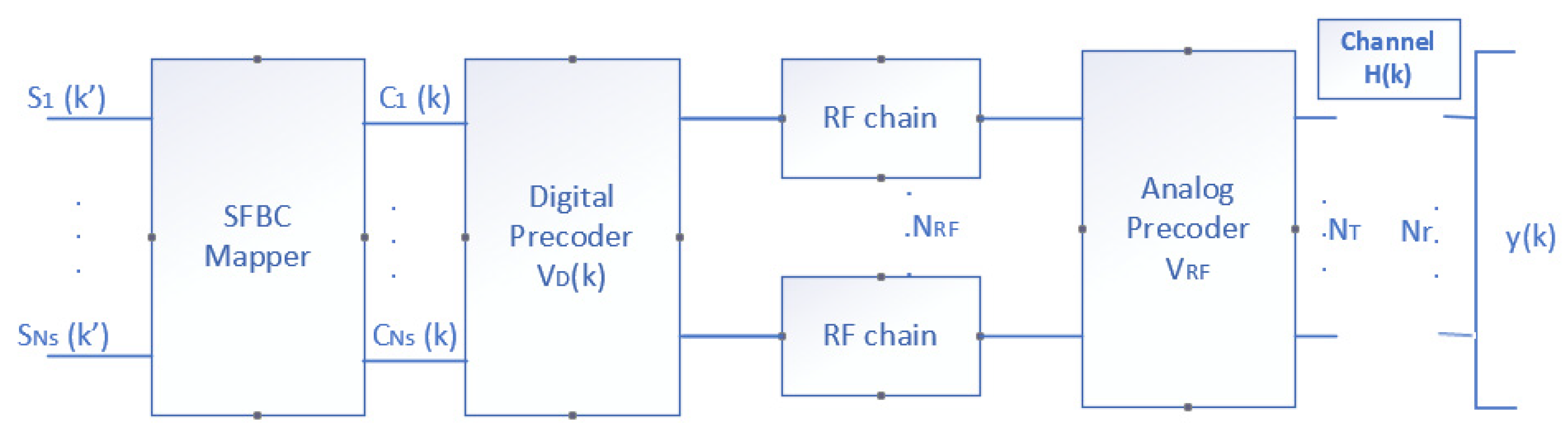
3.1.1. Massive MIMO Hybrid Beamforming (HBF)
3.1.2. Massive MIMO Hybrid Beamforming Applying SFBC (SFBC-HBF)
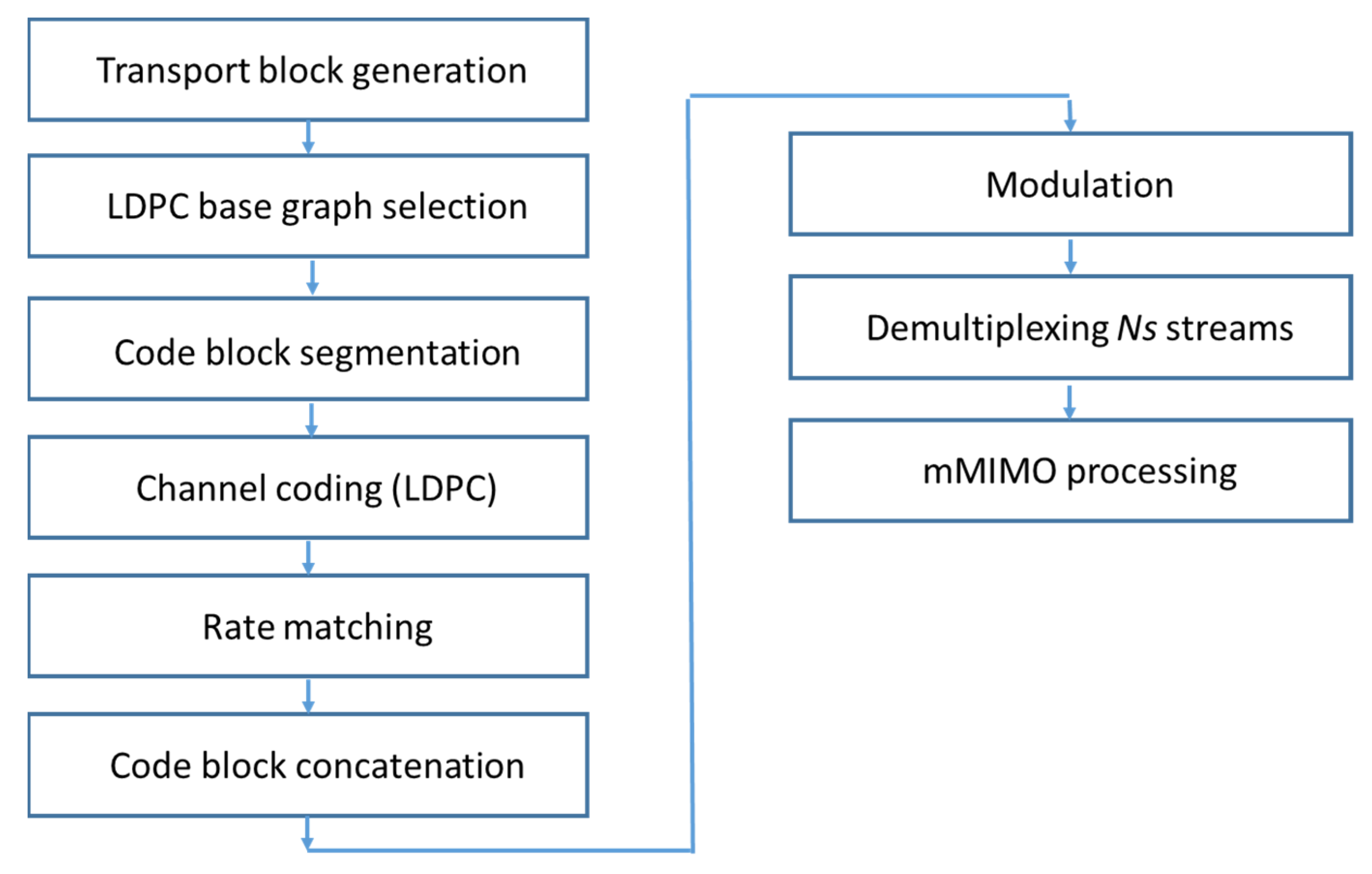
3.2. Physical Layer Parameters
4. Results
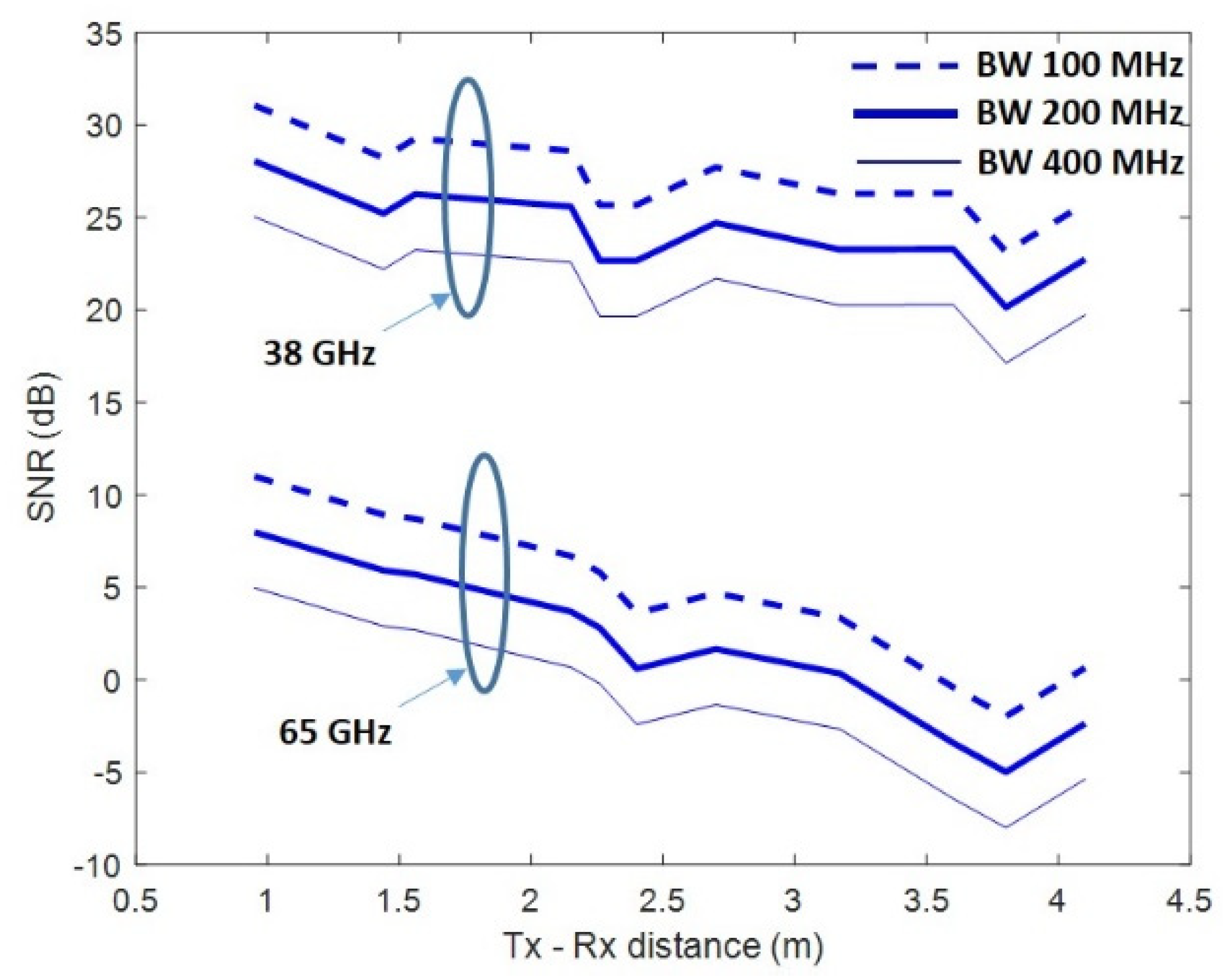
4.1. SNR
4.2. Throughput Analysis
4.2.1. Performance According to Frequency and Bandwidth
4.2.2. Performance According to Algorithm
5. Conclusions and Future Work
Author Contributions
Funding
Conflicts of Interest
References
- David, K.; Berndt, H. 6G vision and requirements: Is there any need for beyond 5G? IEEE Veh. Technol. Mag. 2018, 13, 72–80. [Google Scholar] [CrossRef]
- World Radiocommunication Conference 2019 (WRC-19). Sharm el-Sheikh, Egypt, 28 October–22 November 2019; Available online: https://www.itu.int/en/ITU-R/conferences/wrc/2019/Pages/default.aspx (accessed on 10 May 2022).
- Tripathi, S.; Sabu, N.V.; Gupta, A.K.; Dhillon, H.S. Millimeter-Wave and Terahertz Spectrum for 6G Wireless. In 6G Mobile Wireless Networks. Computer Communications and Networks; Springer: Cham, Switzerland, 2021. [Google Scholar] [CrossRef]
- Kapovits, A.; Gavras, A.; Cosmas, J.; Ghoraishi, M.; Li, X.; Zhang, Y. Delivery of 5G services indoors—The wireless wire challenge and solutions. Zenodo 2021. [Google Scholar] [CrossRef]
- Swindlehurst, A.L.; Ayanoglu, E.; Heydari, P.; Capolino, F. Millimeter-wave massive MIMO: The next wireless revolution? IEEE Commun. Mag. 2014, 52, 56–62. [Google Scholar] [CrossRef]
- Han, S.; Chih-Lin, I.; Xu, Z.; Rowell, C. Large-scale antenna systems with hybrid analog and digital beamforming for millimeter wave 5G. IEEE Commun. Mag. 2015, 53, 186–194. [Google Scholar] [CrossRef]
- Bogale, T.E.; Le, L.B.; Haghighat, A.; Vandendorpe, L. On the number of RF chains and phase shifters, and scheduling design with hybrid analog-digital beamforming. IEEE Trans. Wireless Commun. 2016, 15, 3311–3326. [Google Scholar] [CrossRef] [Green Version]
- Molisch, A.F.; Ratnam, V.V.; Han, S.; Li, Z.; Nguyen, S.L.H.; Li, L.; Haneda, K. Hybrid beamforming for massive MIMO: A survey. IEEE Commun. Mag. 2017, 55, 134–141. [Google Scholar] [CrossRef] [Green Version]
- Yu, X.; Shen, J.-C.; Zhang, J.; Letaief, K.B. Alternating minimization algorithms for hybrid precoding in millimeter wave MIMO systems. IEEE J. Sel. Topics Signal Process. 2016, 10, 485–500. [Google Scholar] [CrossRef] [Green Version]
- Sohrabi, F.; Yu, W. Hybrid digital and analog beamforming design for large-scale antenna arrays. IEEE J. Sel. Topics Signal Process. 2016, 10, 501–513. [Google Scholar] [CrossRef] [Green Version]
- Sohrabi, F.; Yu, W. Hybrid analog and digital beamforming for mmWave OFDM large-scale antenna arrays. IEEE J. Sel. Areas Commun. 2017, 35, 1432–1443. [Google Scholar] [CrossRef] [Green Version]
- Lin, T.; Cong, J.; Zhu, Y.; Zhang, J.; Letaief, K.B. Hybrid beamforming for millimeter wave systems using the MMSE criterion. IEEE Trans. Commun. 2019, 67, 3693–3708. [Google Scholar] [CrossRef] [Green Version]
- Suyama, S.; Okuyama, T.; Nonaka, N.; Asai, T. Recent Studies on Massive MIMO Technologies for 5G Evolution and 6G. In Proceedings of the IEEE Radio and Wireless Symposium (RWS), Las Vegas, NV, USA, 16–19 January 2022. [Google Scholar]
- Gao, X.; Wu, X.; Zhang, Z.; Liu, D. Low Complexity Joint User Scheduling and Hybrid Beamforming for mmWave Massive MIMO Systems. In Proceedings of the IEEE 31st Annual International Symposium on Personal, Indoor and Mobile Radio Communications, London, UK, 31 August–3 September 2020. [Google Scholar]
- Ibrahim, M.S.; Konar, A.; Sidiropoulos, N.D. Fast Algorithms for Joint Multicast Beamforming and Antenna Selection in Massive MIMO. IEEE Trans. Signal Process. 2020, 68, 1897–1909. [Google Scholar] [CrossRef] [Green Version]
- You, L.; Gao, X.; Li, G.Y.; Xia, X.-G.; Ma, N. BDMA for Millimeter-Wave/Terahertz Massive MIMO Transmission With Per-Beam Synchronization. IEEE J. Sel. Areas Commun. 2017, 35, 1550–1563. [Google Scholar] [CrossRef] [Green Version]
- Alouzi, M.; Chan, F.; D’Amours, C. Sphere Decoding for Millimeter Wave Massive MIMO. In Proceedings of the IEEE 90th Vehicular Technology Conference, Honolulu, HI, USA, 22–25 September 2019. [Google Scholar]
- Hong, W.; Jiang, Z.H.; Yu, C.; Zhou, J.; Chen, P.; Yu, Z.; Zhang, H.; Yang, B.; Pang, X.; Jiang, M.; et al. Multibeam Antenna Technologies for 5G Wireless Communications. IEEE Trans. Antennas Propag. 2017, 65, 6231–6249. [Google Scholar] [CrossRef]
- Wang, Y.; Zou, W. Low Complexity Hybrid Precoder Design for Millimeter Wave MIMO Systems. IEEE Commun. Lett. 2019, 23, 1259–1262. [Google Scholar] [CrossRef]
- Obara, T.; Okuyama, T.; Aoki, Y.; Suyama, S.; Lee, J.; Okumura, Y. Indoor and outdoor experimental trials in 28-GHz band for 5G wireless communication systems. In Proceedings of the IEEE 26th Annual International Symposium on Personal, Indoor, and Mobile Radio Communications, Hong Kong, China, 30 August–2 September 2015. [Google Scholar]
- Nonaka, N.; Muraoka, K.; Suyama, S.; Mashino, J.; Kamohara, K.; Sakai, M.; Iura, H.; Nakazawa, M.; Okumura, Y. Indoor Experimental Trial in High SHF Wide-Band Massive MIMO Hybrid Beamforming. In Proceedings of the IEEE 90th Vehicular Technology Conference, Honolulu, HI, USA, 22–25 September 2019. [Google Scholar]
- Zhang, J.; Yu, X.; Letaief, K.B. Hybrid beamforming for 5G and beyond millimeter-wave systems: A holistic view. IEEE Open J. Commun. Soc. 2020, 1, 77–91. [Google Scholar] [CrossRef] [Green Version]
- Lee, K.F.; Williams, D.B. A space-frequency transmitter diversity technique for OFDM systems. Proc. IEEE Global Telecomm. Conf. 2000, 3, 1473–1477. [Google Scholar]
- Torabi, M.; Jemmali, A.; Conan, J. Analysis of the performance for SFBC-OFDM and FSTD-OFDM schemes in LTE systems over MIMO fading channels. Int. J. Adv. Netw. Serv. 2014, 7, 1–11. [Google Scholar]
- 3GPP, 5G.; NR. Release 16. 2020. Available online: https://www.3gpp.org/release-16 (accessed on 15 March 2022).
- Anoh, K.; Okorafor, G.N.; Adebisi, B.; Alabdullah, A.; Jones, S.; Abd-Alhameed, R.A. Full-diversity QO-STBC technique for large-antenna MIMO systems. Electronics 2017, 6, 37. [Google Scholar] [CrossRef] [Green Version]
- 3GPP, 5G.; NR. Base Station (BS) Radio Transmission and Reception. Document 3GPP TS38.104 v.16.4.0 Release 16. 2020. Available online: https://www.etsi.org/deliver/etsi_ts/138100_138199/138104/16.04.00_60/ts_138104v160400p.pdf (accessed on 12 May 2022).
- 3GPP, 5G.; NR. Physical Layer Procedures for Data. Document 3GPP TS38.214 v.16.3.0 Release 16. 2020. Available online: https://www.etsi.org/deliver/etsi_ts/138200_138299/138214/16.03.00_60/ts_138214v160300p.pdf (accessed on 12 May 2022).
- 3GPP, 5G.; NR. Multiplexing and Channel Coding. Document 3GPP TS38.212 v.16.3.0 Release 16. 2020. Available online: https://www.etsi.org/deliver/etsi_ts/138200_138299/138212/16.03.00_60/ts_138212v160300p.pdf (accessed on 12 May 2022).
- 3GPP, 5G.; NR. Physical channels and modulation. Document 3GPP TS38.211 v.16.3.0 Release 16. 2020. Available online: https://www.etsi.org/deliver/etsi_ts/138200_138299/138211/16.03.00_60/ts_138211v160300p.pdf (accessed on 12 May 2022).
- Sanchis Borrás, C.; Molina-Garcia-Pardo, J.-M.; Rubio, L.; Pascual-Garcia, J.; Penarrocha, V.; Juan-Llacer, L.; Reig, J. Millimeter wave MISO-OFDM transmissions in an intra-wagon environment. IEEE Trans. Intell. Transp. Syst. 2021, 22, 4899–4908. [Google Scholar] [CrossRef]
- 3GPP, 5G.; NR. User Equipment (UE) Radio Access Capabilities. Document 3GPP TS38.306 v.16.2.0 Release 16. 2020. Available online: https://www.etsi.org/deliver/etsi_ts/138300_138399/138306/16.02.00_60/ts_138306v160200p.pdf (accessed on 12 May 2022).


| Reference | Year | Measurements? | Environment | Summary |
|---|---|---|---|---|
| [13] | 2022 | yes | Outdoor | It shows experimental results at 28 GHz of 256 × 16 mMIMO BS cooperation technologies for mmWave 5GE. |
| [14] | 2020 | no | - | It joins user scheduling and HBF for mmWave massive MIMO. |
| [15] | 2020 | no | - | It joins multicast beamforming and antenna selection for mmWave Massive MIMO. |
| [16] | 2017 | no | - | It presents beam division multiple access (BDMA) with per-beam synchronization (PBS) in time and frequency for mmWave/THz Massive MIMO. |
| [17] | 2019 | no | Outdoor | It applies the SD algorithm to outdoor uniform planar arrays’ (UPAs) hybrid beamforming mmW massive MIMO systems. It outperforms significantly the ZF and MMSE detectors with 16 QAM modulation over the whole range of SNR. |
| [18] | 2017 | no | Outdoor | It provides an overview of the existing multibeam antenna technologies which include the passive multibeam antennas (MBAs) based on quasi-optical components and beamforming circuits, and multibeam phased-array antennas enabled by various phase-shifting methods. |
| [19] | 2019 | no | - | It provides a hybrid precoding design for mmWave massive MIMO systems. It uses a phase pursuit technique. |
| [20] | 2015 | yes | Indoor | It presents an experimental study of 28 GHz band with 800 MHz bandwidth and beamforming based on Massive MIMO; 96 × 8 mMIMO; 16 QAM; EIRP = 53 dBm; 1.2 Gbit/s can be achieved to 3.5 m. |
| [21] | 2019 | yes | Indoor | It presents an experimental study of 28 GHz frequency band with 500 MHz (100 MHz × 5) bandwidth with 16 spatial-multiplexed streams. Number of BS antennas = 256. Adaptive modulation and coding (<256 QAM). EIRP is not indicated; 25 Gbit/s can be achieved to 10 m. |
| Rx Position | 9 | 11 | 8 | 4 | 10 | 7 | 5 | 6 | 3 | 2 | 1 |
|---|---|---|---|---|---|---|---|---|---|---|---|
| Tx–Rx Distance (m) | 0.95 | 1.44 | 1.56 | 2.15 | 2.26 | 2.40 | 2.70 | 3.17 | 3.60 | 3.80 | 4.10 |
| 38 GHz | 65 GHz | |
|---|---|---|
| VNA output power (dBm) | −25 | 5 |
| Intermediate frequency filter (Hz) | 100 | 10 |
| Number of points | 8192 | 2048 |
| Measured frequency band (GHz) | 1–40 | 57–66 |
| Strategy to separate Tx and Rx antennas | Pre and post amplified EMCORE opto-converters | Cable and two 25 dB amplifiers |
| MCS | Modulation | Codification (Coding Rate × 1024) |
|---|---|---|
| 4 | 4 QAM | 602 |
| 10 | 16 QAM | 658 |
| 19 | 64 QAM | 873 |
| 27 | 256 QAM | 948 |
| BW (MHz) | RBs | Number of Subcarriers (N) (RBs × 12) |
|---|---|---|
| 100 | 66 | 792 |
| 200 | 132 | 1584 |
| 400 | 264 | 3168 |
| Band (GHz) | MCS/Algorithm | BW (MHz) | Th (Gbit/s) | Max. Distance (m) | Min. SNR (dB) |
|---|---|---|---|---|---|
| 65 | 4/HBF | 100 | 0.17 | 2.26 | 3.9 |
| 200 | 0.34 | 1.56 | 3.9 | ||
| 400 | 0.68 | 0.95 | 3.9 | ||
| 4/SFBC + HBF | 100 | 0.08 | 3.60 | −1.3 | |
| 200 | 0.17 | 3.17 | −2.2 | ||
| 400 | 0.34 | 2.70 | −2.7 | ||
| 10/HBF | 100 | 0.37 | 1.56 | 8.6 | |
| 200 | 0 | - | - | ||
| 400 | 0 | - | - | ||
| 10/SFBC + HBF | 100 | 0.18 | 2.26 | 5.0 | |
| 200 | 0.37 | 1.56 | 5.8 | ||
| 400 | 0.22 | 0.95 | 4.9 | ||
| 38 | 19/HBF | 100 | 0.74 | 4.10 | 14.9 |
| 200 | 1.48 | 4.10 | 15.3 | ||
| 400 | 2.97 | 4.10 | 15.4 | ||
| 19/SFBC + HBF | 100 | 0.37 | 4.10 | 9.3 | |
| 200 | 0.74 | 4.10 | 9.8 | ||
| 400 | 1.48 | 4.10 | 9.7 | ||
| 27/HBF | 100 | 1.07 | 4.10 | 21.9 | |
| 200 | 2.15 | 3.60 | 21.2 | ||
| 400 | 4.30 | 2.15 | 21.4 | ||
| 27/SFBC + HBF | 100 | 0.53 | 4.10 | 14.7 | |
| 200 | 1.07 | 4.10 | 14.9 | ||
| 400 | 2.15 | 4.10 | 14.9 |
Publisher’s Note: MDPI stays neutral with regard to jurisdictional claims in published maps and institutional affiliations. |
© 2022 by the authors. Licensee MDPI, Basel, Switzerland. This article is an open access article distributed under the terms and conditions of the Creative Commons Attribution (CC BY) license (https://creativecommons.org/licenses/by/4.0/).
Share and Cite
Sanchis-Borrás, C.; Martinez-Ingles, M.-T.; Molina-Garcia-Pardo, J.-M. Massive MIMO Indoor Transmissions at 38 and 65 GHz Applying Novel HBF Techniques for 5G. Sensors 2022, 22, 3716. https://doi.org/10.3390/s22103716
Sanchis-Borrás C, Martinez-Ingles M-T, Molina-Garcia-Pardo J-M. Massive MIMO Indoor Transmissions at 38 and 65 GHz Applying Novel HBF Techniques for 5G. Sensors. 2022; 22(10):3716. https://doi.org/10.3390/s22103716
Chicago/Turabian StyleSanchis-Borrás, Concepción, Maria-Teresa Martinez-Ingles, and Jose-Maria Molina-Garcia-Pardo. 2022. "Massive MIMO Indoor Transmissions at 38 and 65 GHz Applying Novel HBF Techniques for 5G" Sensors 22, no. 10: 3716. https://doi.org/10.3390/s22103716
APA StyleSanchis-Borrás, C., Martinez-Ingles, M.-T., & Molina-Garcia-Pardo, J.-M. (2022). Massive MIMO Indoor Transmissions at 38 and 65 GHz Applying Novel HBF Techniques for 5G. Sensors, 22(10), 3716. https://doi.org/10.3390/s22103716