Abstract
We address the accuracy of wideband direct position estimation of a radio transmitter via a distributed antenna array in 5G cellular systems. Our derivations are based only on the presence of spatially coherent line-of-sight (LoS) signal components, which is a realistic assumption in small cells, especially in the mmWave range. The system model considers collocated time and phase synchronized receiving front-ends with antennas distributed in 3D space at known locations and connected to the front-ends via calibrated coaxial cables or analog radio-frequency-over-fiber links. Furthermore, the signal model assumes spherical wavefronts. We derive the Cramér-Rao bounds (CRBs) for two implementations of the system: with (a) known signals and (b) random Gaussian signals. The results show how the bounds depend on the carrier frequency, number of samples used for estimation, and signal-to-noise ratios. They also show that increasing the number of antennas (such as in massive MIMO systems) considerably improves the accuracy and lowers the signal-to-noise threshold for localization even for non-cooperative transmitters. Finally, our derivations show that the square roots of the bounds are two to three orders of magnitude below the carrier wavelength for realistic system parameters.
1. Introduction
Recently, there has been a growing interest in massive multiple-input multiple-output (MIMO) systems [1] and millimeter-wave communication (mmWave) technology [2,3,4,5,6,7]. These systems are already finding their place in future 5th generation (5G) cellular systems. A very important application of 5G systems is indoor localization and tracking [8]. Their key objective is to achieve a localization accuracy of about [9], which is satisfactory for location-based services in cellular systems. In this paper, we aim to obtain the limits of the accuracy of these systems and answer the question of whether, in theory, it is possible to achieve localization accuracy significantly better than the carrier wavelength. The vision is that if such localization accuracy is possible, one could exploit it for location-aided communications. We derived the Cramér–Rao bounds (CRBs) for models that admit only LoS signal components. We addressed two implementations of the system: (a) with deterministic sequences known to the receiver system and (b) with random Gaussian sequences.
The analysis of localization accuracy is important for various reasons [10]. They include location-aided communication (LAC) and coordinated multipoint (CoMP) transmission. For example, CRBs describe local properties for CoMP, and they are much more important than integer carrier wavelength ambiguity. The authors in [11] analyze the performance limits of multiple source localization for known and unknown signals and propose an iterative localization method that breaks the search down into multiple single-source searches. By analyzing the CRB with simulations, one can show that exploiting the coherence between different signal snapshots at the same receiver improves localization accuracy [12]. We explore a different kind of coherence than in [12]—the coherence between signals in different receiving channels in the same signal segment (snapshot). The CRBs for 2D localization of a transmitter that is time-synchronized to the receiving system in a spatially non-coherent scenario with dense multipath propagation is derived in [13].
Few papers have addressed localization in spatially coherent scenarios, and much less the accuracy bounds of such localization. In [14] (RFID—radio frequency identification), Refs. [15,16] (passive source localization), and [17] (MIMO radars—active target localization), the authors have shown that exploiting the carrier phase coupling between all receiving antennas in spatially coherent settings can noticeably increase the localization accuracy. Among these papers, the method in [14] achieves the best precision, which is of the carrier wavelength. According to the experimental results in [2], the range (mmWave) has great potential for spatially coherent localization, because the non-line-of-sight (NLoS) components are at least below the LoS component. Methods for passive wideband localization in spatially coherent setups have been proposed in [18], but CRBs for them have not been addressed yet.
In [19], the authors analyze an object inside a reverberation cavity where a wave is reflected a large number of times before arriving at a sensor (NLoS dominant over LoS). An artificial neural network then infers the object’s location from amplitude-only measurements. It was shown that a high dwell time of the wave inside the cavity (the number of reflections) can lower the error even below the carrier wavelength ( of the wavelength). In scenarios that we analyze, we do not rely on a large number of reflections in the area of interest for two reasons—the absorption in the air can have a significant impact on NLoS components in the mmWave band (see [20]) and, besides indoor cells (such as conference rooms, restaurants), we are also interested in small outdoor cells (squares, parks, and so on). Instead, we depend on LoS components (the NLoS components are either negligible or separable from the LoS ones—separable in time thanks to the bandwidth, or separable in space thanks to orthogonal spatial signatures). Note that, even in a small cell/area, the NLoS components with a large number of reflections can have a long propagation distance through the air, which entails that the absorption can be a large source of attenuation for them. As mentioned above, Ref. [2] reported measurements at and showed that the NLoS components were at least below the LoS component. In addition to the mentioned environments (small indoor/outdoor cells/areas), we are interested in the mmWave range of frequencies primarily (especially around ), where the antennas are small and can be packed more densely, which is suitable for indoor implementations.
In [21], it has been found that the estimation accuracy based on TDoA could significantly be increased by exploiting the carrier phase of arrival. This suggests that the localization accuracy could also considerably benefit from the carrier phases in spatially coherent settings. Algorithms for direct wideband coherent localization of a cooperative transmitter by distributed phased antenna arrays have been reported in [22]. Their performance approaches the CRB, and they solve the ambiguity problem inherent to coherent localization in distributed massive MIMO. There are also direct wideband coherent methods for localization of a non-cooperative transmitter via a distributed antenna array in environments with multipath propagation and interference [18].
In [23], the authors analyzed error bounds for uplink and downlink 3D localization in 5G mmWave systems with an antenna array at the base station, as well as at the user terminal. In the studied scenario, the localization parameters were the directions of departure and arrival. Unlike this setting, ours has a base station array whose antennas are distributed throughout the cell and the localization parameters are the coordinates of a selected user antenna (a user terminal can have more than one antenna).
Numerically less expensive methods for LoS localization in a massive MIMO ultra-dense network are proposed in [24]. They take into account the curvature of the wavefront at the base station arrays (spherical vs. planar). In addition to this curvature, unlike in [24], in this paper, we also consider (1) other useful information due to spatial coherence, and (2) the spatial-wideband effect [25,26]. The localization in our paper is suitable for networks with centralized processing of signals received by distributed antennas such as C-RAN networks [27]. In accordance with [28], we used a physical model for the LoS components and a stochastic model for the NLoS components.
In this paper, we derive the CRBs of localization of an arbitrarily wideband stationary radio frequency (RF) transmitter (Tx) in a spatially coherent scenario (such as the one in [18]). The receiving channels are phase- and time-synchronized, but time synchronization between the Tx and the receiving system is not required, unlike for ToA-based methods [17]. The wavefronts are spherical (the planar wave assumption is not used), contrary to the scenario in [15]. The signals are arbitrarily wideband in the sense that any two TDoAs across the receiving array may differ by more than the reciprocal of the bandwidth. The processing of the received signals is coherent; we exploit the phase differences between all the receiving channels for estimation.
We show that the CRBs are inversely proportional to the squared carrier frequency, and their square roots are two to three orders of magnitude below the carrier wavelength for usual system parameters, as opposed to non-coherent signal scenarios/algorithms, where the ranging/localization CRB is inversely proportional to the squared effective signal bandwidth. Moreover, we show that the CRB is inversely proportional to the square of the signal-to-noise ratio (SNR) for low SNRs when the transmitted sequence is random Gaussian and inversely proportional to the SNR for high SNRs, as well as for known sequences (for any SNR). Finally, we found that the CRB is inversely proportional to the number of samples used for estimation.
The localization system can use an unknown-sequence method (a method suited to random signals) to localize a non-cooperative source in the area of interest, that is completely independent from the system, or a known-sequence method to localize cooperative terminals, especially if they are a part of the communication network that also performs this localization (see different methods in [18]). Known-sequence-based methods can be numerically more complex, but they provide a processing gain which suppresses all interference orthogonal to the searched sequence (similar to CDMA (code-division multiple access) systems). We point out that a system can choose to use unknown-sequence methods in both cases. From the perspective of information theory and attainable accuracy, of interest in this paper; if the localization system knows the sequence, then it has more information at its disposal to localize the source. The latter is reflected in the lower error bounds, as shown in this paper.
This paper follows the research direction of extremely large aperture arrays (a group of antennas distributed in a large area that work coherently), [29], and analyzes them as an enabler for highly accurate 3D positioning. The results presented in this paper are a contribution to the idea of using distributed coherent massive MIMO systems as a component (enabling technology) of future 6G wireless networks [30].
The paper is organized as follows. In the next section, we explain the system and signal model used for deriving the CRBs. In Section 3, we present the main derivation results of the paper, and in Section 4, we provide some numerical results obtained from the derived CRBs. In the last section, we provide concluding remarks and directions for future research. In Appendix A, we explain in detail the derivation of the CRBs when the receiving system knows which sequence/waveform the transmitter uses, whereas in Appendix B, we present the derivation details for random transmitted signals.
In the paper, we use the notation given in Table 1.

Table 1.
Symbols and their meaning.
Note that, for the most part of this paper, we use normalized time and frequency quantities (such as ), whereas we use quantities in physical units (non-normalized, such as ) only when necessary. The reason for this decision is that the transition between the analog and the digital domain is then trivial (, when ).
2. System Model
2.1. The Setup
A single stationary transmitter, , is at an unknown location . A distributed stationary receiving antenna array has M elements/channels, , , where the th antenna is at a known location , as in Figure 1.
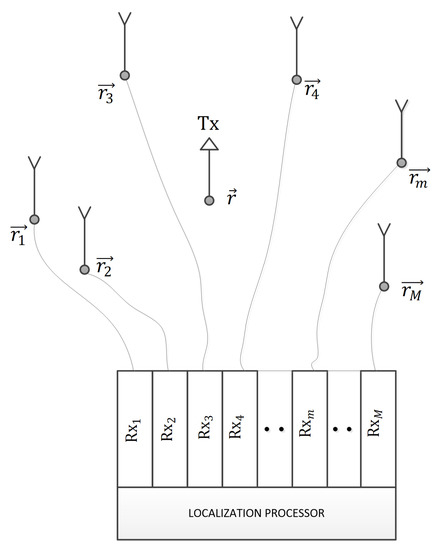
Figure 1.
The system model.
When the distances between adjacent antennas in an array are of the order of , where is the carrier wavelength, we call the array a collocated or classical array. If some of the antennas are separated by many wavelengths, we call such an array distributed. Note that a distributed array does not have to contain only independent (single) antennas, but it may also contain collocated arrays (as its subarrays). It may be cheaper to build a distributed array from prefabricated subarrays (with densely packed, i.e., collocated, antennas in each one) and to multiplex the signals from the antennas of the same subarray through a single cable. (This might especially be convenient at higher frequencies.)
Next, we define the spatial coherence of a signal component (such as an LoS component) from a transmitter Tx, wherever it may be in a given area of interest, , across a set of receiving (Rx) antennas, . We say that the spatial coherence exists, if the difference, denoted by , in the distances from Rx antennas m and ℓ to the Tx implies that the difference in the phase of that component at these two Rx antennas is equal to , for any , where is the carrier frequency and is the speed of propagation in that medium. Note that this is a weaker condition than the medium being homogenous and isotropic. It is weaker because only the phase differences are required to follow this law and only for signals coming from inside of . Furthermore, note that spatial coherence is more likely to exist in smaller cells, and especially indoors. Most importantly, note that spatial coherence is a property of the propagation medium only—it has nothing to do with the front-ends or the cables of the Rx system.
We also define coherent localization methods. We call them coherent if they exploit the information in phase differences between signals in each pair of the receiving channels to increase the accuracy of the localization. This requires (a) spatial coherence in the medium and (b) that the Rx channels work coherently (i.e., that they are time-, frequency-, and phase-synchronized). If they do not work coherently, the phases of the received signals may well be scrambled and this information is lost. Non-coherent methods would still work, because they rely only on signal envelopes. There are also semi-coherent methods, which exploit the phase differences between the signals from the same subarray, but not between different subarrays (because, e.g., the subarrays may be far apart from each other, that is, spread out over a large geographical area where spatial coherence does not exist). Note that spatial coherence, in most cases, exists across collocated arrays.
We now define direct localization methods. These methods estimate the location directly from the raw acquired data (the signal samples), whereas indirect methods estimate the location from some intermediate estimates (such as directions of arrival, times of arrival, time differences of arrival, or received signal strengths). Direct methods usually have better performance at the cost of higher numerical complexity and the need for the transference of raw samples to the signal processor. Furthermore, a wideband localization method is able to cope with signals whose bandwidth is large, such that the differences between envelope delays at different Rx antennas may exceed the inverse of the bandwidth.
Next, we draw some comparisons of our model with other models. Our receiving system model is equivalent to the one in [31,32] for a cell-free network, but the propagation model, however, is not. Namely, the network contains antennas, placed over a wide area, which (thanks to synchronization) work coherently to receive signals. Then, the signal processors process these raw signals, but, unlike in [31,32], where the phases in the Rx signals are scrambled, we consider scenarios with spatial coherence of LoS components, which means the information about the Tx location contained in the phases is preserved. The network may have many more antennas, but only a subset of M of them is chosen. It is assumed that the Tx is in LoS conditions with low path loss with each of the M antennas and that there is spatial coherence of the LoS components across this subset (as explained in [18]). Furthermore, this assumption is made for scalability reasons (see, e.g., [33]). The spatial coherence condition allows coherent localization, which in turn, as we will show, can provide a much higher accuracy. The network also chooses a central processing unit that will run a direct localization algorithm on the acquired signals.
A similar comparison can be drawn against the model in [34]. Using the terminology from [34], we have a number of antennas in a distributed antenna system spread over the area of interest, grouped into remote antenna units (RAUs), where the RAUs can have different numbers of antennas; each RAU contains one or more antennas. The signals from the antennas are fed to baseband processing units (BPUs), as separate streams, where processing occurs (centralized processing is enabled, i.e., a direct localization algorithm can be run). The main differences are (a) the elements of the channel matrix in [34] are random, whereas we model the LoS components separately (from NLoS) and deterministically, and (b) the symbols transmitted at the same time arrive at the Rx antennas also at the same time (narrowband approximation) [34], whereas we consider wideband signals.
We also describe a contrast with [35], where a large number of low-cost low-power sensors transmit wirelessly short messages to a fusion center. Instead of performing coherent direct localization (which requires raw signals at the fusion center, and, therefore, probably requires wired infrastructure), it can cooperate with a high performance network, which performs coherent localization and advanced wireless communication (a network which we model) to help it detect the presence of mobile transmitters.
For the receiving channels to work coherently, the cables connecting the Rx antennas to their front-ends (Figure 1), together with the front-ends themselves, should either induce equal delays (including phase delays) in the signals or the deviations should be compensated for in preprocessing (this is a more likely and a more flexible solution). The IQ (in-phase-quadrature-phase) demodulators should use a local carrier from a common source (frequency-synchronization), the A/D converters should have a common clock, and the corresponding samples should have the same indices (timestamps) (time-synchronization). Readers interested in practical implementations of synchronization methods are referred to [36]. The Rx system receives a signal segment of N complex samples (N in-phase samples as real plus N samples from the quadrature-phase branch as imaginary) from each channel (starting, of course, from the same sample index in each channel). The signal processor then runs a localization algorithm on that segment (which contains samples). The SNRs are defined for each channel, and they are expected to decrease with the square of the distance from the Tx to an Rx antennas, but we allow them to have any values (deviations could happen because the polarizations are not aligned perfectly, for example; especially if the antennas are distributed in 3D). The system, of course, chooses a carrier frequency and a bandwidth appropriate for the band it wants to monitor (to perform localization in).
Note that the Tx does not need to be either time- or phase-synchronized with the receiving system. This means that even noncooperative transmitters can be localized. If one hopes to estimate the location with accuracy better than the carrier wavelength, then the positions of the receiving antennas have to be determined with even better accuracy before the localization algorithm is executed.
2.2. Signal Model
The transmits an RF signal (approximately) bandlimited to , where is the carrier frequency in Hz and B is the signal bandwidth in Hz. The signal received at the th antenna at a distance from , bandlimited to , is sampled at the Nyquist rate and is represented in a complex form as
where ; is a real-valued attenuation factor for the LoS component, ; is the sequence/waveform; the term models all NLoS components; and are the normalized angular and natural carrier frequencies, respectively; the unknown value models the asynchronism between the system and the (we use, as a reference, the time axis); is the propagation time from Tx to , where and is the Euclidean norm; the normalized propagation speed is , where ; there are NLoS paths to the th antenna with complex-valued coefficients and propagation times ; represents noise; the acquired samples are .
Note that and are fractional dimensionless values (the propagation time delays do not have to be integer multiples of the sampling interval) and that the sequence/waveform is defined on the entire (continuous) range because it has been transformed into a continuous waveform inside the .
Unlike the signal model in [1,37], the signal model in this paper is spatially wideband. Furthermore, the steering vectors are modeled implicitly by for each individual Rx antenna. Besides the spatial-wideband effect, this also models the curvature of the wavefronts, which cannot be neglected due to the size of the subarrays compared to the area of interest. Furthermore, in contrast to [1,37], the coefficients are real-valued, thanks to the spatial coherence of the LoS components. Note that the coefficients for the NLoS components may have any phase. In [25,26], it is argued that modeling the spatial-wideband effect is important even for collocated massive arrays and that it is critical for distributed systems.
We scale the signal , in a preprocessing step, by , because the signal-to-noise ratios (SNRs) and noise powers are considered to be known to the receiver. Thereby, the useful signals in all the receiving channels have the same powers. Then, we have
where are the (scaled) NLoS components and is a circular-complex zero-mean Gaussian random process with variance , , independent across time samples and channels and independent from the waveform . Then, the SNR in channel m is defined by
The propagation attenuations are modeled by , but the model considers that no information about the transmitter location is contained in the attenuations. In practice, location estimation based on phases is more robust than the location estimation based on attenuations.
Our objective is to find the CRBs of the estimates of unknown parameters for the cases of (a) known and (b) random sequences. In the former case, the unknown parameters are and in the latter, . Let us recall that the Tx is not time-synchronized with the Rx system. Therefore, the parameter (the shift between the Tx and Rx time axes) is unknown to the signal processor. Even though we are not interested (in this context) in obtaining an estimate of (we are only interested in estimating —the Tx location), must be modeled as an unknown and, therefore, as a part of in case (a). Otherwise, an estimation algorithm could exploit this information to produce a better estimate than could be possible (on average) with the given model (and that would mean that the error bound would be different, too).
In contexts outside of the scope of this paper, an estimate of might not be irrelevant. On the contrary, if the Rx system (such as a base station or a group of them) were synchronized to the universal time, and it sent its estimate of to the Tx (the terminal), the Tx could adjust its clock to match the universal time as well (as an additional service, the system could provide to the terminal).
Another important thing to note is that, in case (b), regardless of how good or bad an estimation algorithm is, it would be unable to estimate at all. An intuitive explanation could be: If , , and were likely estimates of , , and the location, then the estimates , , and would be equally likely, for any , no mater how large is, so the error would be unbounded. A formal explanation is as follows: the Fisher information matrix (see the next section) in case (b), if we chose would be singular, and we need to invert it to obtain the CRB, which would mean that the CRB would tend to infinity.
3. Cramér-Rao Bounds
The authors in [23,38] provide CRBs for localization when the user terminal and the base station each have a single collocated (small aperture) antenna array. They show that, when the number of antennas grows, the CRBs of the LoS component parameters tend to the appropriate LoS-only CRBs, because the LoS components become separable from the NLoS ones, thanks to the channel sparsity in mmWave. In accordance with that, we derive the CRBs when . This allows us to quantify the impact of the location information in the LoS components on the attainable localization accuracy, regardless of the model for the NLoS components (whether they are modeled as random or deterministic and whether they are changing more slowly of quickly). Even if the NLoS components are not negligible in some scenarios in practice, the LoS-only CRBs are useful for selecting the resolution of a search grid for localization methods that use grids. If the system designer cannot predict how much the NLoS components would degrade the accuracy, it seems logical to use the resolution appropriate for the case without that degradation.
3.1. Known Sequences (Cooperative Transmitter)
This case corresponds to a scenario where a base station allocates a sequence for a cooperative user terminal. The terminal then transmits the sequence so that the base station can localize the terminal. From the assumptions about in (2), we deduce that and have zero-mean Gaussian distributions with variance , , where and denote the real and imaginary parts of the argument, respectively. It holds then, that , where stands for the expectation operator. Furthermore, the probability density function (PDF) of a single time sample is
All the observations are given by the vector
. The PDF of is given by
and thus, the loglikelihood function, , is
The Fisher information matrix (FIM) of the unknown parameters is defined by
After taking the first partial derivatives of with respect to the unknown parameters given in , we get expressions of the form
where (if we use the symbol to denote the first derivative)
Then, after taking the second partial derivatives of , we obtain
where is a deterministic function without an impact on the final result (as explained in Appendix A). These expressions depend on , which we treat as random variables (not their realizations). After applying the expectation operator to them, we get FIM elements of the form
where the multiplication factor is given by
and is common to all of the FIM elements. It is interesting to note that the first term in takes into account the impact of the information in the carrier phase on the error bound, whereas the second term (the derivative of the sequence, ) takes into account the bandwidth. Finally, we need to invert the FIM. The elements on the main diagonal of are the error bounds for , x, y, and z, in that order. The bound on the mean squared localization error is then the sum of the elements , , and of for 3D and the sum of and for 2D localization. Appendix A provides the steps of this derivation in more detail.
Let be the SNR of a channel whose antenna is away from the transmitter. Based on the derived expressions for the FIM elements, we obtain that the CRB approximately depends on , the carrier frequency, and the number of samples is as follows:
3.2. Random Gaussian Sequences (Non-Cooperative Transmitter)
This case corresponds to a scenario where a base station tries to localize a (possibly non-cooperative) terminal transmitting a signal unknown to the base station (probably with a compact spectrum, e.g., OFDM). We reiterate that in our derivation for random sequences, the beginning of the period of the transmitted sequence, , is unknown, but irrelevant for the localization. The reason is that a time-shifted white Gaussian process has the same statistical properties as its version without a time shift. The CRBs derived here are approximate, since the signal is not periodic with period N and the DFT-based time shift is cyclic.
Contrary to the scenario with known sequences, here, all of the -acquired time samples are dependent in pairs, which makes it inconvenient to form the joint distribution. Namely, if in (1) were an integer, say 17, then , as well as in (2), would depend only on . However, in reality, is not an integer, but say , and therefore depends on all of ( being random variables and being a function of them). The same is true for (for that particular channel m)—each of them depends on all . It would be easier if we had groups of variables such that the groups are independent from each other. Then, the total joint PDF would be a simple product of the PDFs of each group individually.
An idea for addressing this is to transform the received signals into the frequency domain (using DFT). We perform the DFT on the time domain vector to get a vector of DFT components, and we repeat this for each Rx channel m, . This way, we obtain a new statistical sample, which contains frequency samples, instead of the old one, which contains time samples, but the amount of information in the new one and in the old one is the same (they are equivalent). Next, at a given frequency with index k, we can group the k-th DFT component from each of the Rx channels into an M-element vector . We show that these N groups (random vectors) are independent from each other (exactly what we were looking for). Finally, all that remains is to find the PDF of each group and calculate their product. We proceed by explaining these steps in more detail in the following text. As a convention, we will use the symbol to denote DFT spectra.
The DFT spectra of the signal and noises are
where denotes the DFT operator.
In order to express time shifts in the spectral domain realistically, let the discrete frequency be in the range .
The reason for this choice is that the DFT components in the complex baseband domain need to correspond correctly to the RF frequencies in the range . If we chose k to be in (as in classical signal processing), that would correspond to the frequencies in the range , which would be in conflict with the model. Since , relying on the properties of the DFT operator defined in (16), we have
where . Since the noise signals and the unknown useful signal are white (uncorrelated time samples) stationary complex Gaussian random processes, their DFT components, and , are also i.i.d. (independent and identically distributed) complex Gaussian [39]. The fact that the samples at different frequencies are independent is a very convenient property when we need to find the joint PDF—a property we do not have in the time domain. Note that the time samples and are independent because, in the model, we consider that the sampling is performed at the Nyquist frequency. This, however, does not restrict the analysis in this paper to such systems. Even if a system performs oversampling (which has some advantages), it can reduce the sampling frequency to the Nyquist frequency later in the digital domain. Regardless, the amount of information is the same (in the band of interest), which is important for the analysis of precision. Therefore, the model is general (it holds for both types of systems). To summarize in a more formal way, the properties of and imply that , , , and have Gaussian distributions, i.e., , and . Furthermore, the processes and are also independent, as are the random variables and (and similarly and ) for . Finally, the real components are independent from the imaginary components.
Instead of having time samples in the statistical sample, we can compute and use the DFT samples of the received signals. So, the entire statistical sample (containing complex scalars from the frequency domain) is
Note that the m-th row of the matrix is the DFT spectrum of the signal from the m-th channel and that the columns (viewed as random vectors) are independent from each other. For the PDF of , we can write
because the random variables for different frequencies are independent [39]. Also, we have
where are independent.
In Appendix B, first we show that we can write the loglikelihood as
where , , and where and are real and
We note that and A do not depend on .
The FIM of the parameters is given by
Taking the first partial derivatives of with respect to the unknown parameters given in , we get expressions of the form
Then, taking the second partial derivatives yields expressions of the form
Next, we apply the expectation operator to the second derivatives (treating the DFT components as random variables) to get the FIM elements, of the form
where the multiplication factor
is common to all of the FIM elements. Since the FIM in the random sequence case does not have a row/column that corresponds to , the bound on the mean squared localization error is simply the trace of for 3D and the sum of the elements and for 2D localization. Appendix B provides the steps of this derivation in more detail.
Based on the expressions for the FIM elements, the CRB approximately depends on , the carrier frequency, and the number of samples as follows:
4. Discussion
In this section, we present experimental results that provide further insights on the localization performance of the studied system. Figure 2 shows a 3D slice representation of the CRB for 3D localization inside a room of size , with 18 antennas on each wall and the ceiling (90 in total), marked with triangles, for , , , and a random Gaussian sequence. For convenience, the parameters are also displayed in Table 2, case 1. In the figure, we plotted as a function of the 3D space, where is the carrier wavelength. We imagined that a distributed array would come in prefabricated panels with subarrays of antennas for easy installation. So, we modeled four smaller subarrays (but still with inter-antenna distances considerably larger than ) on the walls, and a larger one (with a larger aperture) on the ceiling.
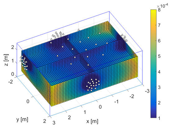
Figure 2.
of 3D localization inside a room of size with 18 antennas on each wall and the ceiling, all marked with triangles. The obtained CRB is for a random Gaussian sequence and parameters , , .
Table 2.
Parameters used for the numerical results.
Note that the cuboid frame is only a rough model of the room—There would be furniture and people inside and the walls are not expected to be completely flat in practice. Furthermore, they would not be ideal reflective surfaces, but the wave would penetrate the walls to an unknown depth, depending on their conductance and other parameters, changing the carrier phase by a significant amount. Using the information in NLoS components in coherent localization would be much more challenging than LoS components, because ray-tracing-based localization algorithms would have to know the depth, whereas fingerprinting-based methods might require the frequent retraining of their databases (since variations in the phases have to be taken into account here). However, this remains an interesting topic for plausibility studies in future research—Could the obstacles be anchored in space with high enough precision as well (as the Rx antennas are) to enable the gains of coherent localization from their reflected components? This is outside the scope of this paper, so we discard the NLoS components in this error-bound analysis.
Figure 3 shows the CRB for a distributed array with five randomly placed antennas for 2D localization in the plain of the array, for , , and a random Gaussian sequence (Table 2, case 2). Since the CRB is much lower inside the array aperture, this suggests that a distributed array should be placed in such a way that its aperture encompasses the area where one expects the transmitters.
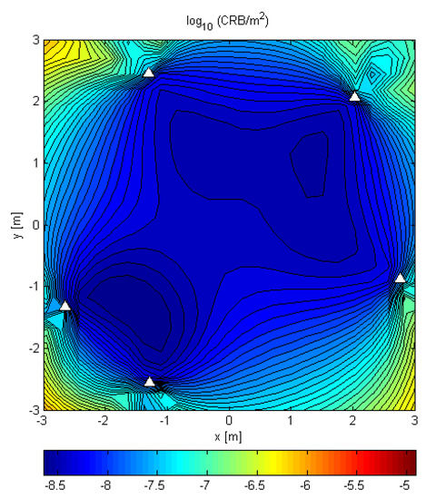
Figure 3.
CRB for 2D localization by five randomly placed antennas in the plain of the array. The locations of the antennas are marked by triangles. The obtained CRB is for a random Gaussian sequence and parameters and .
It is worth noting that both of these example antenna array geometries were chosen to be irregular. An impact on localization performance could be seen as analogous to classical arrays, where nonuniform or sparse arrays perform better than uniform ones for a given number of antennas. In [40], a uniform antenna array with a large number of elements was optimized by reducing the number of used elements greatly (a more cost-effective solution), effectively creating a sparse array with performance comparable to that of the original array. The optimization of an array geometry is also out of scope here, but is an interesting topic for further research. Our idea is that this analysis would also be applicable to geometries that would be set up as ad hoc and then the antenna positions measured.
In Figure 4, we present how the 90% quantile of depends on , , and N, for a random Gaussian sequence (Table 2, case 3). The plots show how the accuracy of localization improves with frequency, N, and SNR. They also demonstrate the advantage of using mmWave because the increased frequency of the carrier allows for higher localization accuracy. The results for known sequences are similar.
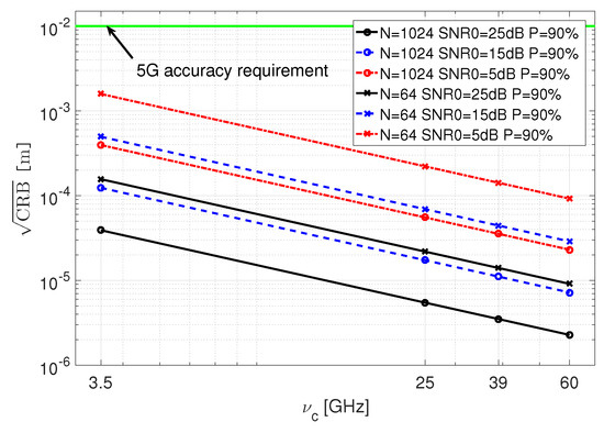
Figure 4.
The quantile of vs. for a Gaussian sequence and , for different and N.
It is also worth investigating how the CRBs depend on the number of antennas, M. Since the effect of relative placement of antennas to each other and the effect of increasing M are coupled, we have chosen to evaluate the CRBs for a uniform square distributed array with , , , and antennas (so ). The arrays were attached to the ceiling of a room and the CRBs were evaluated in a square of size and centered directly below the array, in a horizontal plane, for , , (Table 2, case 4). We analyzed a constant aperture and a constant antenna distance scenario. In the former, the array’s aperture was kept at , whereas in the latter, the adjacent antennas were retained at from each other, effectively making the arrays identical in both setups. Figure 5 compares the CRBs of the arrays in the constant aperture and Figure 6, in the constant antenna distance scenario.
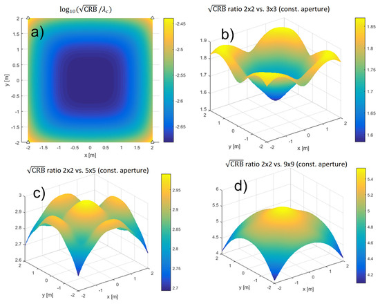
Figure 5.
The CRBs for different array sizes in the constant aperture scenario. The square root of the CRB, normalized by the carrier wavelength, for the array is shown in (a). The ratios of on one hand and , , and on the other are shown in (b), (c), and (d), respectively.
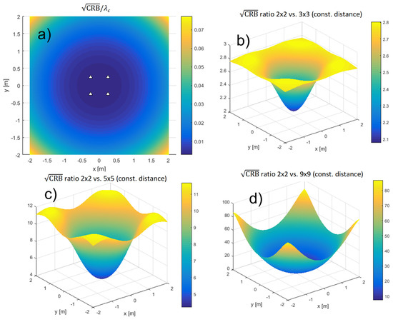
Figure 6.
The CRBs for different array sizes in the constant antenna distance scenario. The square root of the CRB, normalized by the carrier wavelength, for the array is shown in (a). The ratios of on one hand and , , and on the other are shown in (b), (c), and (d), respectively.
When we average the CRBs over the possible locations of the transmitter in the square of the experiment, we obtain the results depicted in Figure 7. They show how the CRBs change with M and comparing them with the ideal ∼1/M and ∼1/ dependencies. This shows how much increasing the number of antennas improves the accuracy of localization.
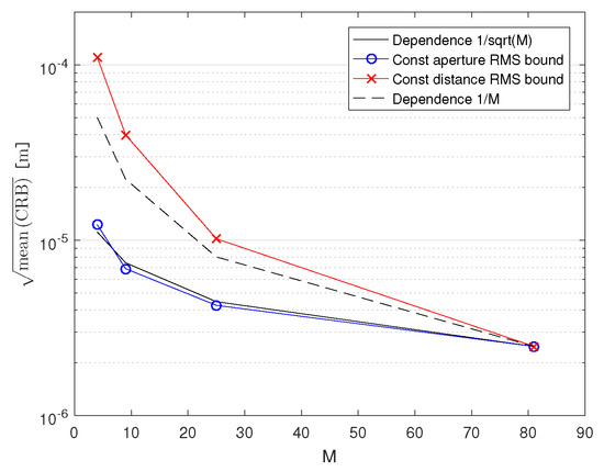
Figure 7.
Dependence of the CRB on the number of antennas, M.
We have also evaluated the CRB curves as a function of (recall that is the SNR of a channel whose antenna is 1 m away from the transmitter) for random Gaussian sequences and known sequences (Table 2, case 5). Again, the results are obtained by averaging the CRBs for locations of the transmitter over locations in the square of the experiment. The results for the and arrays are shown in Figure 8. They suggest that increasing the number of antennas from 4 to 81 produces a gain of approximately . The results also show the advantage of using mmWave massive MIMO systems because the localization can successfully be performed in low SNR conditions (low transmitted power in the mmWave range), even for unknown sequences (non-cooperative scenarios). In [18], the authors present additional results for CRBs and localization algorithms evaluated for different sets of parameters, including different array geometries.
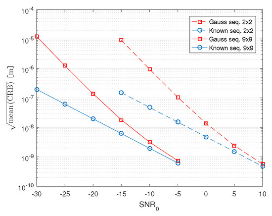
Figure 8.
Dependence of the CRB, averaged over space, on .
Finally, we point out that in coherent direct localization, besides the main lobe of the criterion function of the localization algorithm, there usually exists a number of high sidelobes (the space between them is on the order of the carrier wavelength), so that some estimates are placed on these lobes, degrading the absolute error. This is called the (integer wavelength) ambiguity problem (for further details, please see [18]). However, for distributed beamforming (which is one of the important applications of coherent localization), this absolute error is irrelevant, whereas the error within the main lobe (the distance of its local maximum to the true location) determines its performance. This error is much smaller than the absolute one and is reflected in the CRB (which describes only local behavior). For this reason, the ambiguity problem is outside the scope of this paper. Some possible solutions, though, are mentioned in [18].
5. Conclusions
In this paper, we have addressed the performance limits of direct wideband coherent 3D localization in distributed mmWave massive MIMO for 5G cellular systems. In the derivation of the limits, we assume only the presence of spatially coherent line-of-sight signal components. We also assume collocated time- and phase-synchronized receiving front-ends with antennas distributed at known locations. The results for known and random Gaussian signals show that the CRB is inversely proportional to the squared carrier frequency. For a typical indoor setting and realistic system parameters (, , ), the square root of the CRB is smaller than in of the space. These results suggest important advantages of massive MIMO for 5G systems. Namely, one can preprocess the signals at the base station array to focus energy at the selected user antenna in the downlink and, conversely, to increase the gain in the uplink. This shifts the focus from location-based services to the location aided communication concept. This entails that coherent localization in LoS scenarios, typical for small cells in mmWave range, has the potential to improve the capacity considerably and the overall performance of 5G massive MIMO systems with distributed antennas. The results also show that the studied systems are especially suited for coherent localization due to high accuracy and the ability to perform localization in low SNR conditions (low radiated power), even with non-cooperative transmitters. The ambiguity problem of coherent localization can be solved in a number of ways, e.g, by optimizing the antenna geometry or by using signals from antenna subarrays distributed in the cell.
Finally, we provide some topics for future research. In practice, the propagation conditions inside a cell may vary over time, so it is desirable for a localization system to implement different methods (with different strengths and weaknesses), such as RSS and coherent ones. It would be valuable to compare their performance and design schemes that activate appropriate methods based on the detected conditions.
Furthermore, optimization of antenna array geometries based on different criteria is of interest. One criterion is the accuracy, but the main accuracy gain seems to be achieved by placing the array so that the transmitters are inside its aperture. Another criterion is the reduction of the ambiguity problem, which can easily happen in coherent localization when the number of antennas is small. This is of interest in applications where absolute error is important (traffic collision prevention, automated robot and drone movement control).
A challenging direction of research is an error analysis in conditions with more pronounced NLoS components and the possibility to leverage information in strong reflections to improve coherent localization.
The exploration of a fair comparison between the error bounds of RSS (received signal strength; i.e., amplitude only) and coherent localization (from this paper) is also important. RSS localization puts no additional requirements on the hardware. To make the comparison fair, it would have to be carried out in conditions suitable for both types. Namely, RSS localization is robust against synchronization errors and a lack of spatial coherence in the medium. On the other hand, coherent localization is robust against deviations in the received power from a law with a given path loss exponent. This is especially important for 3D localization, where not all of the antenna polarizations would be aligned, so that it could even happen that an Rx antenna closer to the Tx has a weaker received signal power than another Rx antenna farther away.
Another interesting topic for further research is the possibility of using reconfigurable intelligent surfaces (RIS) to aid coherent localization for increased accuracy (the use of a RIS in non-coherent localization was already reported in [19]). Namely, if a localization system could measure very accurately the position of a RIS and if it controls (or knows) the phase changes that the RIS induces in the signal component, it reflects from a transmitter (that needs to be localized). Then, a coherent localization algorithm might be able to use such an NLoS component in addition to the LoS component for better performance (especially if the transmitter is well outside the aperture of the Rx antenna array). The paper [41] presents challenges and opportunities for using RISs in localization.
Author Contributions
Conceptualization, N.V.; methodology, N.V.; software, N.V.; validation, P.M.D. and M.E.; formal analysis, N.V.; investigation, N.V., M.E., and P.M.D.; writing, original draft preparation, N.V., M.E.; writing, review and editing, N.V., M.E., and P.M.D.; visualization, N.V. and M.E.; supervision, P.M.D. All authors have read and agreed to the published version of the manuscript.
Funding
This work was partially supported by the Serbian Ministry of Education, Science and Technological Development project TR32028 and by the US NSF under Award CCF-1618999. The APC was funded by Vlatacom Institute, Belgrade, Serbia.
Institutional Review Board Statement
Not applicable.
Informed Consent Statement
Not applicable.
Data Availability Statement
Not applicable.
Conflicts of Interest
The authors declare no conflict of interest. The funders had no role in the design of the study; in the collection, analyses, or interpretation of data; in the writing of the manuscript, or in the decision to publish the results.
Abbreviations
The following abbreviations are used in the manuscript:
| 2D | 2-dimensional |
| 3D | 3-dimensional |
| 5G | Fifth generation |
| 6G | Sixth generation |
| BPU | Baseband processing unit |
| C-RAN | Cloud radio access networks |
| CDMA | Code-division multiple access |
| CoMP | Coordinated multipoint |
| CRB | Cramér-Rao bound |
| DFT | Discrete Fourier transform |
| FIM | Fisher information matrix |
| i.i.d. | Independent and identically distributed |
| IQ | In-phase-quadrature-phase |
| LAC | Location aided communication |
| LoS | Line-of-sight |
| MIMO | Multiple-input multiple-output |
| mmWave | Millimeter-wave |
| NLoS | Non-line-of-sight |
| Probability density function | |
| RAU | Remote antenna unit |
| RF | Radio frequency |
| RFID | Radio frequency identification |
| RFoF | Radio-frequency-over-fiber |
| RIS | Reconfigurable intelligent surface |
| RSS | Received signal strength |
| SNR | Signal-to-noise ratio |
| TDoA | Time difference of arrival |
| ToA | Time of arrival |
Appendix A. CRB Derivation-Known Sequences
We rewrite the loglikelihood function from (6), , i.e.,
The FIM is given by
In the derivation, we use the identity , where (·)* denotes complex conjugation. Note also that since
we can write
Define
where (·)′ denotes the first derivative. Then, the first derivatives of the loglikelihood are
If we define , then for the second derivatives we obtain
where , , are deterministic functions, whose expressions are not given for brevity. They are all deterministic, and each of them is multiplied by the term whose expectation is equal to zero, and therefore, their values have no impact on the result in the next step.
Then, for the first element of the FIM we write
If we define as
after some simple derivation, we get
because shifting a signal in time does not change its energy. Note that does not depend on m. Then and the rest of the FIM elements can be expressed in compact forms respectively as
The CRBs for the individual components are given by
We define by the error in locating the transmitter. For the bound of its mean squared value, we write
where is the cofactor of the th element of . For simplicity of notation, we will call this bound just the (transmitter location) CRB.
If the transmitter’s z-coordinate is known (which corresponds to 2D localization), the corresponding FIM, , is obtained by removing the last row and column of the FIM for the 3D case, . Namely,
and the CRB for 2D localization is
Let the quantity be defined as the SNR value in a channel whose antenna would be away from the transmitter. If the signal power decreases with the square of the distance from the transmitter, and if the noise has equal power across the channels prior to scaling by , starting from the derived expressions above, , , and the assumption that is large in the sense that , it can be shown that the CRBs approximately depend on , the carrier frequency, and the number of samples as follows: (Actually, . So, the expression holds if B is constant, since . In addition, the dependence on B also exists in c.)
Appendix B. CRB Derivation—Random Gaussian Sequences
We start with writing the joint PDF . This random vector is a function of independent random variables (one for the useful signal, , and M for the noise, ). We obtain the joint PDF by integrating over all the possible values of the signal random variable, . If we denote and , then
where is the value of the PDF of the complex random variable evaluated at . After some rearranging, we obtain
where (which are real), and are defined by
The FIM is
Note that , A do not depend on . For the log likelihood, we write further
Note that the first two terms of do not depend on , but the third term does. In the sequel, we use the following identities: . For the first derivatives of , we obtain
The second derivatives of the loglikelihood are
The expressions for , , , and are analogous. Note that the only random variables in the second derivatives of are the frequency components . If the expectation operator is applied to the second derivatives, there will be terms of the form
and
These equalities are used to derive the elements of the FIM. The derivation is somewhat tedious but straightforward and yields
where
The CRBs are then given by
The bound on the mean squared error of the transmitter’s location estimate is then
where is the cofactor of the th element of . If the transmitter’s z-coordinate is known (the 2D localization case), the last row and column of are removed to obtain the FIM for the 2D case,
So, the CRB for 2D localization is
Under similar assumptions as in the known sequence scenario, starting from the derived expressions, and with the approximations
it can be shown that the CRB approximately depends on , the carrier frequency, and the number of samples as follows:
References
- Garcia, N.; Wymeersch, H.; Larsson, E.G.; Haimovich, A.M.; Coulon, M. Direct localization for massive MIMO. IEEE Trans. Signal Process. 2017, 65, 2475–2487. [Google Scholar] [CrossRef]
- Xu, H.; Kukshya, V.; Rappaport, T.S. Spatial and temporal characterization of 60 GHz indoor channels. In Proceedings of the Vehicular Technology Conference, Boston, MA, USA, 24–28 September 2000; Volume 1, pp. 6–13. [Google Scholar]
- Torkildson, E.; Madhow, U.; Rodwell, M. Indoor millimeter wave MIMO: Feasibility and performance. IEEE Trans. Wirel. Commun. 2011, 10, 4150–4160. [Google Scholar] [CrossRef]
- Haneda, K.; Gustafson, C.; Wyne, S. 60 GHz spatial radio transmission: Multiplexing or beamforming? IEEE Trans. Antennas Propag. 2013, 61, 5735–5743. [Google Scholar] [CrossRef]
- El-Sayed, H.; Athanasiou, G.; Fischione, C. Evaluation of localization methods in millimeter-wave wireless systems. In Proceedings of the IEEE 19th International Workshop on Computer Aided Modeling and Design of Communication Links and Networks (CAMAD), Athens, Greece, 1–3 December 2014; pp. 345–349. [Google Scholar]
- Olivier, A.; Bielsa, G.; Tejado, I.; Zorzi, M.; Widmer, J.; Casari, P. Lightweight indoor localization for 60-GHz millimeter wave systems. In Proceedings of the 13th Annual IEEE International Conference on Sensing, Communication, and Networking (SECON), London, UK, 27–30 June 2016; pp. 1–9. [Google Scholar]
- Lemic, F.; Martin, J.; Yarp, C.; Chan, D.; Handziski, V.; Brodersen, R.; Fettweis, G.; Wolisz, A.; Wawrzynek, J. Localization as a feature of mmWave communication. In Proceedings of the Wireless Communications and Mobile Computing Conference (IWCMC), Paphos, Cyprus, 5–9 September 2016; pp. 1033–1038. [Google Scholar]
- Dardari, D.; Closas, P.; Djurić, P.M. Indoor Tracking: Theory, Methods, and Technologies. IEEE Trans. Veh. Technol. 2015, 64, 1263–1278. [Google Scholar] [CrossRef]
- Yassin, A.; Nasser, Y.; Awad, M.; Al-Dubai, A.; Liu, R.; Yuen, C.; Raulefs, R.; Aboutanios, E. Recent advances in indoor localization: A survey on theoretical approaches and applications. IEEE Commun. Surv. Tutor. 2016, 19, 1327–1346. [Google Scholar] [CrossRef]
- Di Taranto, R.; Muppirisetty, S.; Raulefs, R.; Slock, D.; Svensson, T.; Wymeersch, H. Location-aware communications for 5G networks: How location information can improve scalability, latency, and robustness of 5G. IEEE Signal Process. Mag. 2014, 31, 102–112. [Google Scholar] [CrossRef]
- Chen, J.C.; Hudson, R.E.; Yao, K. Maximum-Likelihood Source Localization and Unknown Sensor Location Estimation for Wideband Signals in the Near-Field. IEEE Trans. Signal Process. 2002, 50, 1843–1854. [Google Scholar] [CrossRef]
- Li, J.; Yang, L.; Guo, F.; Jiang, W. Coherent summation of multiple short-time signals for direct positioning of a wideband source based on delay and Doppler. Digit. Signal Process. 2016, 48, 58–70. [Google Scholar] [CrossRef]
- Wilding, T.; Grebien, S.; Mühlmann, U.; Witrisal, K. Accuracy Bounds for Array-Based Positioning in Dense Multipath Channels. Sensors 2018, 18, 4249. [Google Scholar] [CrossRef] [PubMed]
- Scherhäufl, M.; Pichler, M.; Stelzer, A. UHF RFID localization based on phase evaluation of passive tag arrays. IEEE Trans. Instrum. Meas. 2015, 64, 913–922. [Google Scholar] [CrossRef]
- Oispuu, M.; Nickel, U. 3D passive source localization by a multi-array network: Noncoherent vs. coherent processing. In Proceedings of the International ITG Workshop on Smart Antennas, Bremen, Germany, 23–24 February 2010; pp. 300–305. [Google Scholar]
- Hadaschik, N.; Sackenreuter, B.; Schäfer, M.; Faßbinder, M. Direct positioning with multiple antenna arrays. In Proceedings of the International Conference on Indoor Positioning and Indoor Navigation, Calgary, AB, Canada, 13–16 October 2015; pp. 1–10. [Google Scholar]
- Godrich, H.; Haimovich, A.M.; Blum, R.S. Target localization accuracy gain in MIMO radar-based systems. IEEE Trans. Inf. Theory 2010, 56, 2783–2803. [Google Scholar] [CrossRef]
- Vukmirović, N.; Erić, M.; Janjić, M.; Djurić, P.M. Direct Wideband Coherent Localization by Distributed Antenna Arrays. Sensors 2019, 19, 4582. [Google Scholar] [CrossRef] [PubMed]
- del Hougne, M.; Gigan, S.; del Hougne, P. Deeply Sub-Wavelength Localization with Reverberation-Coded-Aperture. arXiv 2021, arXiv:2102.05642. [Google Scholar]
- Rappaport, T.S.; Murdock, J.N.; Gutierrez, F. State of the Art in 60-GHz Integrated Circuits and Systems for Wireless Communications. Proc. IEEE 2011, 99, 1390–1436. [Google Scholar] [CrossRef]
- Janjić, M.; Vukmirović, N.; Erić, M. TDOA, Frequency and Phase Offsets Estimation Taking Into Account Carrier Phase of Arrival. Radioengineering 2017, 26, 1143–1150. [Google Scholar] [CrossRef]
- Vukmirović, N.; Janjić, M.; Djurić, P.M.; Erić, M. Position estimation with a millimeter-wave massive MIMO system based on distributed steerable phased antenna arrays. EURASIP J. Adv. Signal Process. 2018, 2018, 33. [Google Scholar] [CrossRef] [PubMed]
- Abu-Shaban, Z.; Zhou, X.; Abhayapala, T.; Seco-Granados, G.; Wymeersch, H. Error Bounds for Uplink and Downlink 3D Localization in 5G Millimeter Wave Systems. IEEE Trans. Wirel. Commun. 2018, 17, 4939–4954. [Google Scholar] [CrossRef]
- Han, K.; Liu, Y.; Deng, Z.; Yin, L.; Shi, L. Direct Positioning Method of Mixed Far-field and Near-field Based on 5G Massive MIMO System. IEEE Access 2019, 7, 72170–72181. [Google Scholar] [CrossRef]
- Wang, B.; Gao, F.; Jin, S.; Lin, H.; Li, G.Y. Spatial- and Frequency-Wideband Effects in Millimeter-Wave Massive MIMO Systems. IEEE Trans. Signal Process. 2018, 66, 3393–3406. [Google Scholar] [CrossRef]
- Wang, B.; Gao, F.; Jin, S.; Lin, H.; Li, G.Y.; Sun, S.; Rappaport, T.S. Spatial-Wideband Effect in Massive MIMO with Application in mmWave Systems. IEEE Commun. Mag. 2018, 56, 134–141. [Google Scholar] [CrossRef]
- Jeong, S.; Simeone, O.; Haimovich, A.; Kang, J. Positioning via direct localisation in C-RAN systems. IET Commun. 2016, 10, 2238–2244. [Google Scholar] [CrossRef]
- Yu, K.; Ottersten, B. Models for MIMO Propagation Channels, A Review. J. Wirel. Commun. Mob. Comput. 2002, 2, 653–666. [Google Scholar] [CrossRef]
- Björnson, E.; Sanguinetti, L.; Wymeersch, H.; Hoydis, J.; Marzetta, T.L. Massive MIMO is a Reality–What is Next? Five Promising Research Directions for Antenna Arrays. Digit. Signal Process. 2019, 94, 3–20. [Google Scholar] [CrossRef]
- Wikström, G.; Peisa, J.; Rugeland, P.; Johansson, N.; Parkvall, S.; Girnyk, M.; Mildh, G.; Da Silva, I.L. Challenges and Technologies for 6G. In Proceedings of the 2020 2nd 6G Wireless Summit (6G SUMMIT), Levi, Finland, 17–20 March 2020; pp. 1–5. [Google Scholar]
- Ngo, H.Q.; Ashikhmin, A.; Yang, H.; Larsson, E.G.; Marzetta, T.L. Cell-free Massive MIMO versus small cells. IEEE Trans. Wirel. Commun. 2017, 16, 1834–1850. [Google Scholar] [CrossRef]
- Nayebi, E.; Ashikhmin, A.; Marzetta, T.L.; Yang, H. Cell-free massive MIMO systems. In Proceedings of the 49th Asilomar Conference on Signals, Systems and Computers (ACSSC), Pacific Grove, CA, USA, 8–11 November 2015; pp. 695–699. [Google Scholar]
- Björnson, E.; Sanguinetti, L. A New Look at Cell-Free Massive MIMO: Making It Practical With Dynamic Cooperation. In Proceedings of the 2019 IEEE 30th Annual International Symposium on Personal, Indoor and Mobile Radio Communications (PIMRC), Istanbul, Turkey, 8–11 September 2019; pp. 1–6. [Google Scholar]
- Wang, D.; Wang, J.; You, X.; Wang, Y.; Chen, M.; Hou, X. Spectral Efficiency of Distributed MIMO Systems. IEEE J. Sel. Areas Commun. 2013, 31, 2112–2127. [Google Scholar] [CrossRef]
- Ciuonzo, D.; Salvo Rossi, P.; Dey, S. Massive MIMO Channel-Aware Decision Fusion. IEEE Trans. Signal Process. 2015, 63, 604–619. [Google Scholar] [CrossRef]
- Yan, H.; Hanna, S.; Balke, K.; Gupta, R.; Cabric, D. Software Defined Radio Implementation of Carrier and Timing Synchronization for Distributed Arrays. In Proceedings of the 2019 IEEE Aerospace Conference, Big Sky, MT, USA, 2–9 March 2019; pp. 1–12. [Google Scholar]
- Garcia, N.; Haimovich, A.M.; Dabin, J.A.; Coulon, M.; Lops, M. Direct Localization of Emitters Using Widely Spaced Sensors in Multipath Environments. In Proceedings of the 2014 48th Asilomar Conference on Signals, Systems and Computers, Pacific Grove, CA, USA, 2–5 November 2014; pp. 695–700. [Google Scholar]
- Wang, Y.; Wu, Y.; Shen, Y. Joint Spatiotemporal Multipath Mitigation in Large-Scale Array Localization. IEEE Trans. Signal Process. 2019, 67, 783–797. [Google Scholar] [CrossRef]
- Whalen, A.D. Detection of Signals in Noise; Academic: Cambridge, MA, USA, 1971. [Google Scholar]
- Buttazzoni, G.; Babich, F.; Vatta, F.; Comisso, M. Geometrical Synthesis of Sparse Antenna Arrays Using Compressive Sensing for 5G IoT Applications. Sensors 2020, 20, 350. [Google Scholar] [CrossRef]
- Wymeersch, H.; He, J.; Denis, B.; Clemente, A.; Juntti, M. Radio Localization and Mapping With Reconfigurable Intelligent Surfaces: Challenges, Opportunities, and Research Directions. IEEE Veh. Technol. Mag. 2020, 15, 52–61. [Google Scholar] [CrossRef]


Publisher’s Note: MDPI stays neutral with regard to jurisdictional claims in published maps and institutional affiliations. |
© 2021 by the authors. Licensee MDPI, Basel, Switzerland. This article is an open access article distributed under the terms and conditions of the Creative Commons Attribution (CC BY) license (https://creativecommons.org/licenses/by/4.0/).