
Mapping of Agricultural Subsurface Drainage Systems Using Unmanned Aerial Vehicle Imagery and Ground Penetrating Radar †


Abstract
1. Introduction
1.1. Research Rationale

1.2. Justification Supporting the Use of GPR and UAV Imagery in Combination
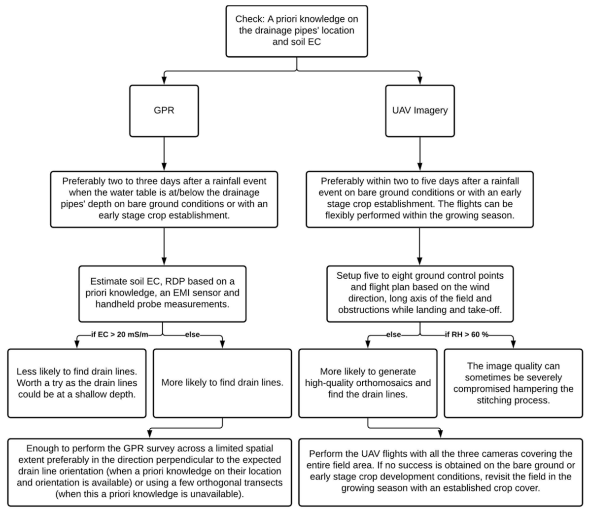
1.3. Research Focus
2. Materials and Methods
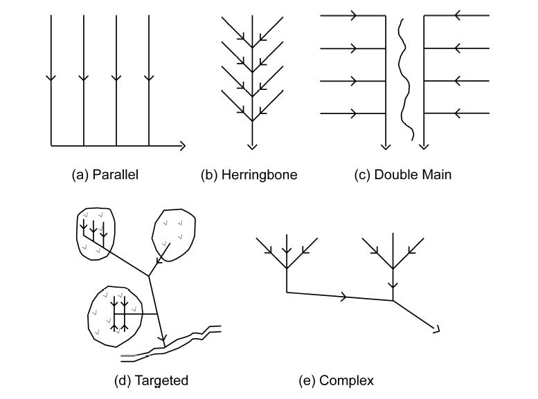
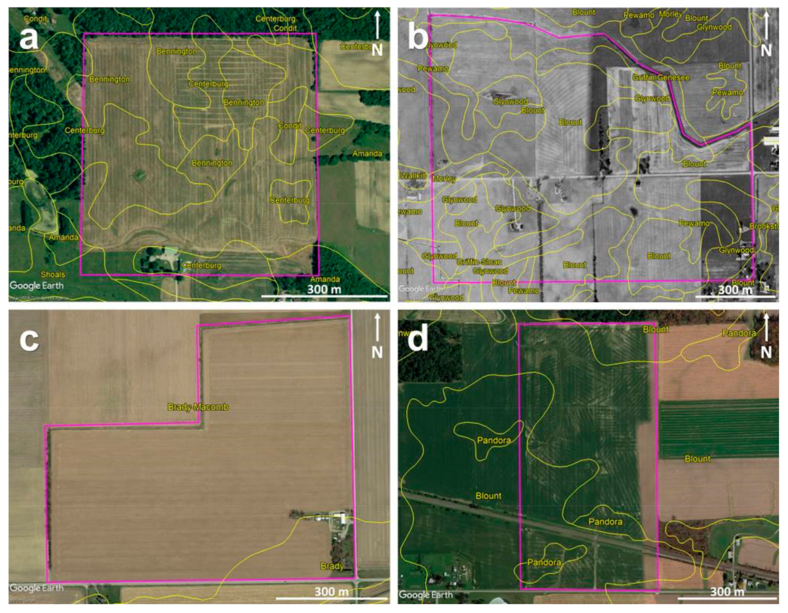
2.1. Study Sites


| Site Name | Soil Types * | Site Conditions | Date of the UAV Surveys and 3 Days’ Prior Rainfall # (mm) | Date of the GPR Surveys and 3 Days’ Prior Rainfall # (mm) |
|---|---|---|---|---|
| Site-1, OH | Silt loam | Bare ground with corn stubble to the west side and soybean stubble to the east side | 6 May 2019 (18.5) | 2–6 May 2019 (18.5) |
| Site 2, MI | Sandy loam, loam, clay loam | Limited and extensive bare ground, respectively, to the north and south of the road with an early-stage soybean and corn crop development (7 May 2018); established cereal ryegrass cover crop (21 May 2019) | 7 May 2018 (1.5); 21 May 2019 (19.9) | 21 May 2019 (19.9) |
| Site 3, MI | Sandy loam, loam | Extensive bare ground (7 May 2018); established soybean crop (12 July 2018); and extensive bare ground (10 December 2019) | 7 May 2018 (3.1); 12 July 2018 (0) | 12 July 2018 (0); 10 December 2019 (5.6) |
| Site 4, OH | Silt loam | Substantial soybean residue on extensive bare ground | 21 June 2019 (44.7) | 21 June 2019 (44.7) |

2.2. UAV Equipment, Survey, and Data Processing
2.2.1. Equipment
2.2.2. Survey Information
2.2.3. Data Processing

| Camera | Sensor | Center Wavelength(s) nm | Bandwidth nm | Resolution cm/Pixel |
|---|---|---|---|---|
| S.O.D.A | RGB * | 450, 520, and 660 | ~300 | 2.8 |
| Sequoia | RGB * | 470, 550, and 660 | ~300 | 3 |
| Green | 550 | 40 | 11 | |
| Red | 660 | 40 | 11 | |
| Red Edge | 735 | 10 | 11 | |
| Near-Infrared | 790 | 40 | 11 | |
| thermoMAP | Thermal Infrared | 10,000 | 3000 | 22 |
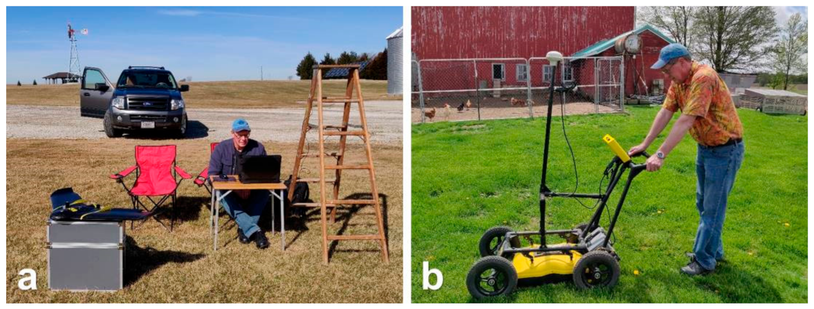
2.3. GPR Equipment, Survey, and Data Processing
2.3.1. Equipment
2.3.2. Survey Information
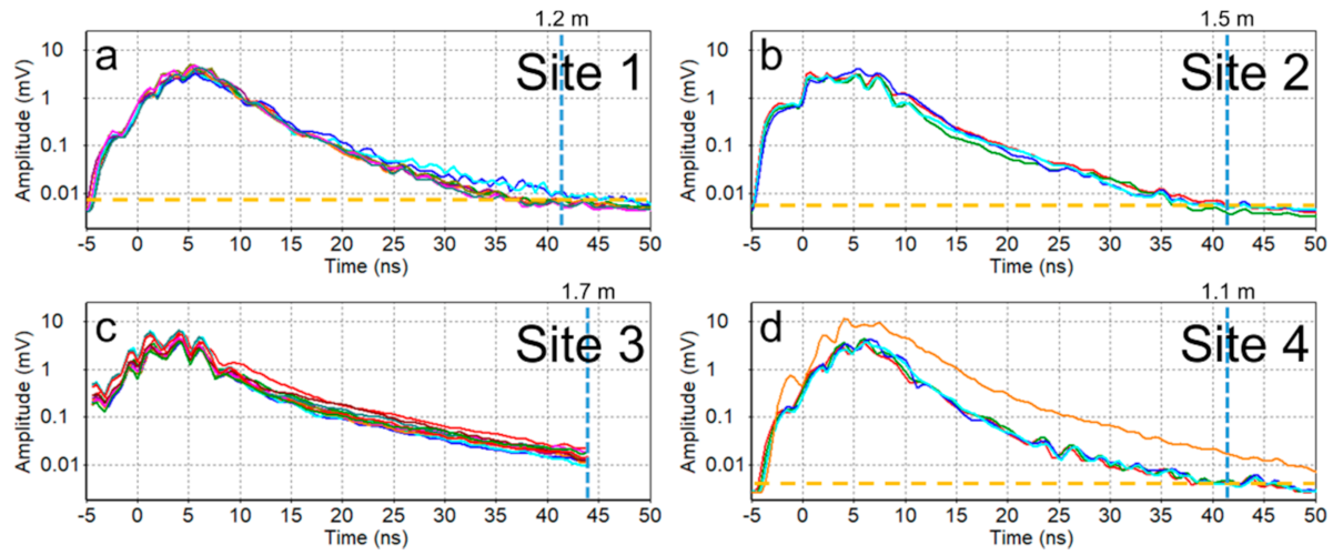
2.3.3. Data Processing
3. Results and Discussion
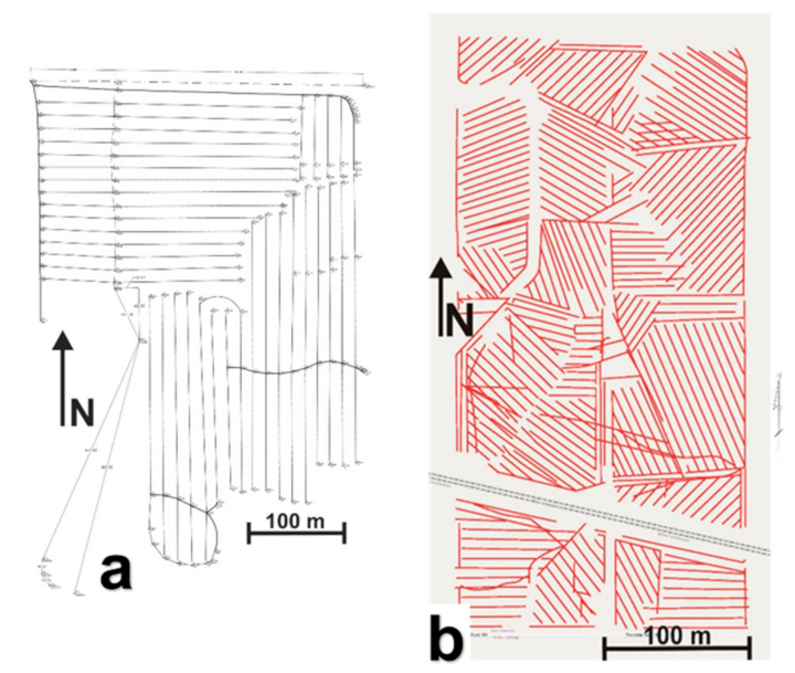
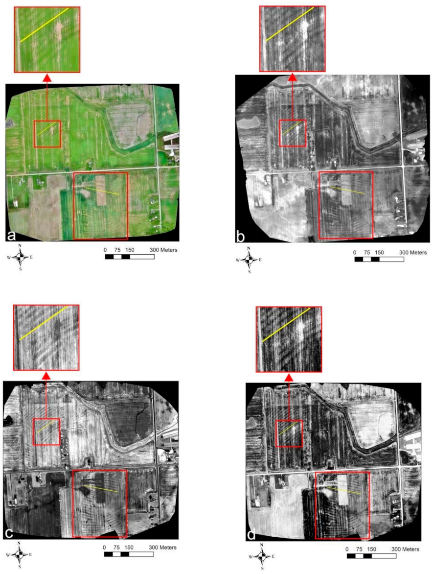
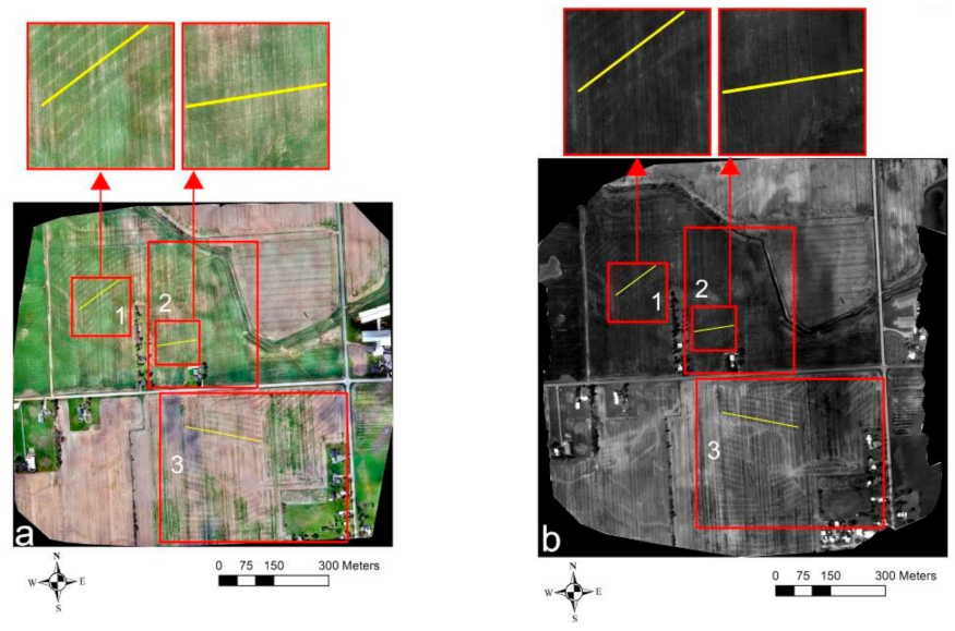
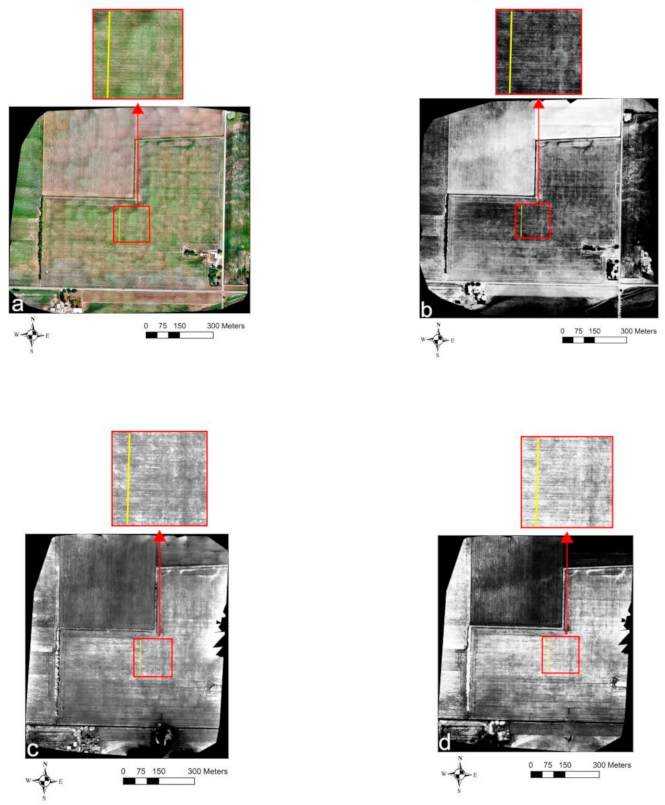
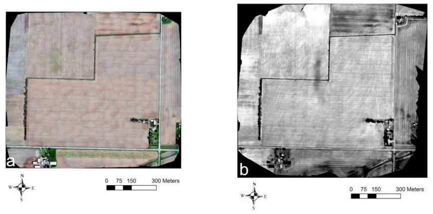
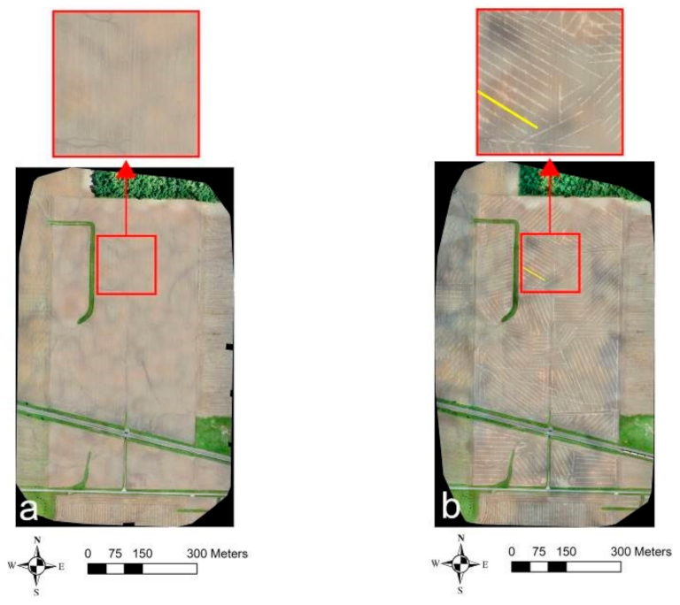
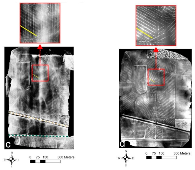
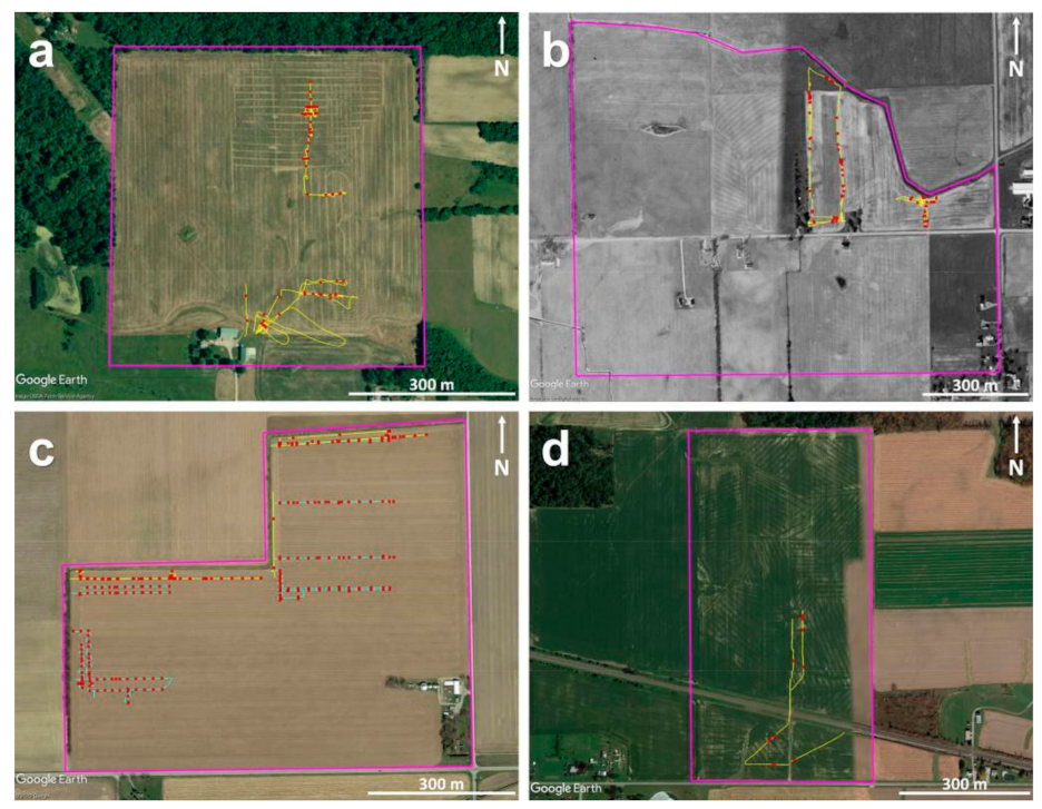
3.1. UAV Results


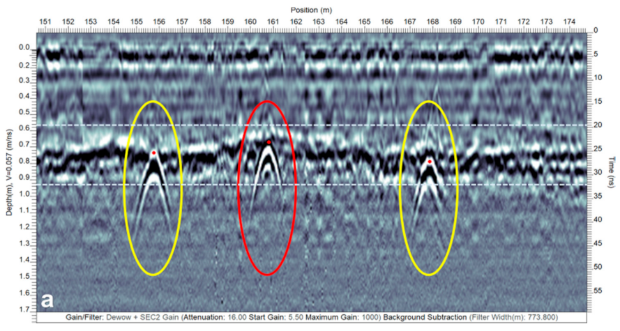
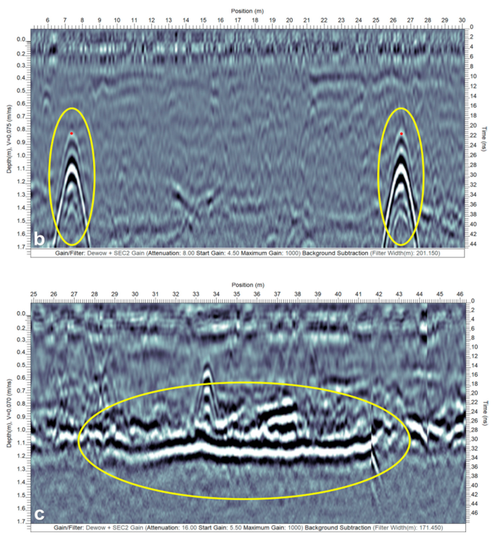
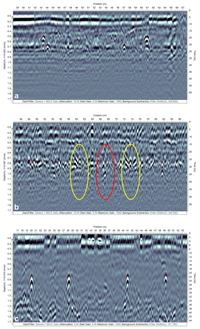
3.2. GPR Results


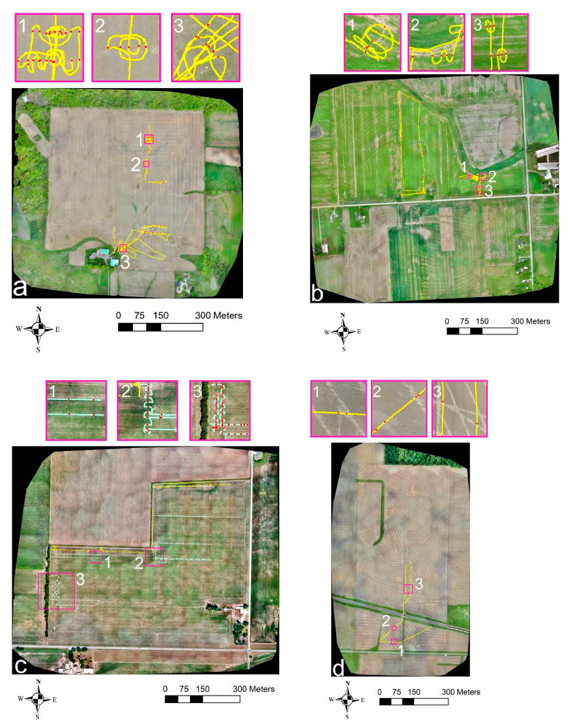
3.3. Complementary Nature of the UAV Imagery and GPR and Combined Interpretation

4. Recommendations and Future Work

5. Conclusions
Supplementary Materials
Author Contributions
Funding
Institutional Review Board Statement
Informed Consent Statement
Data Availability Statement
Acknowledgments
Conflicts of Interest
References
- Skaggs, R.W.; Breve, M.A.; Gilliam, J.W. Hydrologic and water-quality impacts of agricultural drainage. Crit. Rev. Environ. Sci. Technol. 1994, 24, 1–32. [Google Scholar] [CrossRef]
- Fraser, H.; Fleming, R.; Eng, P. Environmental Benefits of Tile Drainage; Prepared for LICO–Land Improvement Contractors of Ontario, Ridgetown College, University of Guelph: Ridgetown, ON, Canada, 2001. [Google Scholar]
- Khand, K.; Kjaersgaard, J.; Hay, C.; Jia, X.H. Estimating Impacts of Agricultural Subsurface Drainage on Evapotranspiration Using the Landsat Imagery-Based METRIC Model. Hydrology 2017, 4, 49. [Google Scholar] [CrossRef]
- Jaynes, D.B.; Colvin, T.S.; Karlen, D.L.; Cambardella, C.A.; Meek, D.W. Nitrate loss in subsurface drainage as affected by nitrogen fertilizer rate. J. Environ. Qual. 2001, 30, 1305–1314. [Google Scholar] [CrossRef]
- Blann, K.L.; Anderson, J.L.; Sands, G.R.; Vondracek, B. Effects of agricultural drainage on aquatic ecosystems: A review. Crit. Rev. Environ. Sci. Technol. 2009, 39, 909–1001. [Google Scholar] [CrossRef]
- King, K.W.; Fausey, N.R.; Williams, M.R. Effect of subsurface drainage on streamflow in an agricultural headwater watershed. J. Hydrol. 2014, 519, 438–445. [Google Scholar] [CrossRef]
- King, K.W.; Williams, M.R.; Macrae, M.L.; Fausey, N.R.; Frankenberger, J.; Smith, D.R.; Kleinman, P.J.A.; Brown, L.C. Phosphorus transport in agricultural subsurface drainage: A review. J. Environ. Qual. 2015, 44, 467–485. [Google Scholar] [CrossRef] [PubMed]
- Erickson, A.J.; Gulliver, J.S.; Weiss, P.T. Phosphate removal from agricultural tile drainage with iron enhanced sand. Water 2017, 9, 672. [Google Scholar] [CrossRef]
- Hua, G.H.; Salo, M.W.; Schmit, C.G.; Hay, C.H. Nitrate and phosphate removal from agricultural subsurface drainage using, laboratory woodchip bioreactors and recycled steel byproduct filters. Water Res. 2016, 102, 180–189. [Google Scholar] [CrossRef] [PubMed]
- Jaynes, D.B.; Isenhart, T.M. Reconnecting Tile Drainage to Riparian Buffer Hydrology for Enhanced Nitrate Removal. J. Environ. Qual. 2014, 43, 631–638. [Google Scholar] [CrossRef]
- Vymazal, J. Removal of nutrients in various types of constructed wetlands. Sci. Total Environ. 2007, 380, 48–65. [Google Scholar] [CrossRef]
- Pugliese, L.; De Biase, M.; Chidichimo, F.; Heckrath, G.J.; Iversen, B.V.; Kjaergaard, C.; Straface, S. Modelling phosphorus removal efficiency of a reactive filter treating agricultural tile drainage water. Ecol. Eng. 2020, 156, 105968. [Google Scholar] [CrossRef]
- Pugliese, L.; Skovgaard, H.; Mendes, L.R.D.; Iversen, B.V. Treatment of agricultural drainage water by surface-flow wetlands paired with woodchip bioreactors. Water 2020, 12, 1891. [Google Scholar] [CrossRef]
- Allred, B.J.; Daniels, J.J.; Fausey, N.R.; Chen, C.; Peters, L.; Youn, H. Important considerations for locating buried agricultural drainage pipe using ground penetrating radar. Appl. Eng. Agric. 2005, 21, 71–87. [Google Scholar] [CrossRef]
- Allred, B.J.; Fausey, N.R.; Peters, L.; Chen, C.; Daniels, J.J.; Youn, H. Detection of buried agricultural drainage pipe with geophysical methods. Appl. Eng. Agric. 2004, 20, 307–318. [Google Scholar] [CrossRef]
- Allred, B.J.; Redman, J.D. Location of agricultural drainage pipes and assessment of agricultural drainage pipe conditions using ground penetrating radar. J. Environ. Eng. Geoph. 2010, 15, 119–134. [Google Scholar] [CrossRef]
- Valipour, M.; Krasilnikof, J.; Yannopoulos, S.; Kumar, R.; Deng, J.; Roccaro, P.; Mays, L.; Grismer, M.E.; Angelakis, A.N. The evolution of agricultural drainage from the earliest times to the present. Sustainability 2020, 12, 416. [Google Scholar] [CrossRef]
- Yannopoulos, S.I.; Grismer, M.E.; Bali, K.M.; Angelakis, A.N. Evolution of the materials and methods used for subsurface drainage of agricultural lands from antiquity to the present. Water 2020, 12, 1767. [Google Scholar] [CrossRef]
- Schwab, G.O.; Fouss, J.L. Drainage materials. In Agricultural Drainage; Skaggs, R.W., van Schilfgaarde, J., Eds.; Agronomy Monograph No. 38; American Society of Agronomy: Madison, WI, USA, 1999; pp. 911–926. [Google Scholar]
- Stuyt, L.; Dierickx, W.; Beltrán, J.M. Materials for Subsurface Land Drainage Systems; Paper No. 60 Rev. 1; Food and Agricultural Organization of the United States: Rome, Italy, 2005. [Google Scholar]
- Strock, J.; Sands, G.; Helmers, M. Subsurface drainage design and management to meet agronomic and environmental goals. In Soil Management: Building a Stable Base for Agriculture; Hatfield, J.L., Sauer, T.J., Eds.; American Society of Agronomy and Soil Science Society of America: Madison, WI, USA, 2011; pp. 199–208. [Google Scholar]
- Nijland, H.; Croon, F.W.; Ritzema, H.P. Subsurface Drainage Practices: Guidelines for the Implementation, Operation and Maintenance of Subsurface Pipe Drainage Systems; ILRI Publication No. 60; Alterra: Wageningen, The Netherlands, 2005. [Google Scholar]
- Rogers, M.B.; Cassidy, J.R.; Dragila, M.I. Ground-based magnetic surveys as a new technique to locate subsurface drainage pipes: A case study. Appl. Eng. Agric. 2005, 21, 421–426. [Google Scholar] [CrossRef]
- Designing a Subsurface Drainage System. Available online: https://extension.umn.edu/agricultural-drainage/designing-subsurface-drainage-system#topography-and-system-layout-1367611 (accessed on 20 April 2020).
- Schwab, G.O.; Frevert, R.K.; Edminster, T.W.; Barnes, K.K. Chapter 14-Subsurface drainage design. In Soil and Water Conservation Engineering, 3rd ed.; John Wiley & Sons: New York, NY, USA, 1981; pp. 314–347. [Google Scholar]
- Allred, B.J.; Wishart, D.; Martinez, L.; Schomberg, H.; Mirsky, S.; Meyers, G.; Elliott, J.; Charyton, C. Delineation of agricultural drainage pipe patterns using ground penetrating radar integrated with a real-time kinematic global navigation satellite system. Agriculture 2018, 8, 167. [Google Scholar] [CrossRef]
- Boniak, R.; Chong, S.; Indorante, S.; Doolittle, J. Mapping golf green drainage systems and subsurface features using ground-penetrating radar. In Proceedings of the Ninth International Conference on Ground Penetrating Radar, Santa Barbara, CA, USA, 12 April 2002; Volume 4758, pp. 477–481. [Google Scholar]
- Chow, T.L.; Rees, H.W. Identification of subsurface drain locations with ground-penetrating radar. Can. J. Soil. Sci. 1989, 69, 223–234. [Google Scholar] [CrossRef]
- Allred, B.J. A GPR agricultural drainage pipe detection case study: Effects of antenna orientation relative to drainage pipe directional trend. J. Environ. Eng. Geoph. 2013, 18, 55–69. [Google Scholar] [CrossRef]
- Koganti, T.; Van De Vijver, E.; Allred, B.J.; Greve, M.H.; Ringgaard, J.; Iversen, B.V. Assessment of a stepped-frequency GPR for subsurface drainage mapping for different survey configurations and site conditions. In Proceedings of the 10th International Workshop on Advanced Ground Penetrating Radar, The Hague, The Netherlands, 8–12 September 2019; pp. 1–7. [Google Scholar]
- Koganti, T.; Van De Vijver, E.; Allred, B.J.; Greve, M.H.; Ringgaard, J.; Iversen, B.V. Mapping of agricultural subsurface drainage systems using a frequency-domain ground penetrating radar and evaluating its performance using a single-frequency multi-receiver electromagnetic induction instrument. Sensors 2020, 20, 3922. [Google Scholar] [CrossRef] [PubMed]
- Thayn, B.J.; Campbell, M.; Deloriea, T. Mapping Tile-Drained Agriculture Land; The Institute for Geospatial Analysis and Mapping (GEOMAP), Illinois State University: Normal, IL, USA, 2011; pp. 1–16. [Google Scholar]
- Verma, A.K.; Cooke, R.A.; Wendte, L. Mapping subsurface drainage systems with color infrared aerial photographs. In Proceedings of the American Water Resource Association Symposium on GIS and Water Resources, Ft. Lauderdale, FL, USA, 22–26 September 1996; pp. 457–466. [Google Scholar]
- Naz, B.S.; Ale, S.; Bowling, L.C. Detecting subsurface drainage systems and estimating drain spacing in intensively managed agricultural landscapes. Agric. Water Manag. 2009, 96, 627–637. [Google Scholar] [CrossRef]
- Tetzlaff, B.; Kuhr, P.; Wendland, F. A new method for creating maps of artificially drained areas in large river basins based on aerial photographs and geodata. Irrig. Drain 2009, 58, 569–585. [Google Scholar] [CrossRef]
- Varner, B.L.; Gress, T.A.; White, S.E. The effectiveness and economic feasibility of image-based agricultural tile maps. In Proceedings of the 6th International Conference on Precision Agriculture and Other Precision Resources Management, Minneapolis, MN, USA, 14–17 July 2002; pp. 1450–1464. [Google Scholar]
- Northcott, W.J.; Verma, A.K.; Cooke, R. Mapping subsurface drainage systems using remote sensing and GIS. In Proceedings of the ASAE Annual International Meeting, Milwaukee, WI, USA, 9–12 July 2000; pp. 1–10. [Google Scholar]
- Møller, A.B.; Beucher, A.; Iversen, B.V.; Greve, M.H. Predicting artificially drained areas by means of a selective model ensemble. Geoderma 2018, 320, 30–42. [Google Scholar] [CrossRef]
- Allred, B.J.; Eash, N.; Freeland, R.; Martinez, L.; Wishart, D. Effective and efficient agricultural drainage pipe mapping with UAS thermal infrared imagery: A case study. Agric. Water Manag. 2018, 197, 132–137. [Google Scholar] [CrossRef]
- Allred, B.J.; Martinez, L.; Fessehazion, M.K.; Rouse, G.; Williamson, T.N.; Wishart, D.; Koganti, T.; Freeland, R.; Eash, N.; Batschelet, A. Overall results and key findings on the use of UAV visible-color, multispectral, and thermal infrared imagery to map agricultural drainage pipes. Agric. Water Manag. 2020, 232, 106036. [Google Scholar] [CrossRef]
- Freeland, R.; Allred, B.; Eash, N.; Martinez, L.; Wishart, D. Agricultural drainage tile surveying using an unmanned aircraft vehicle paired with real-time kinematic positioning-A case study. Comput. Electron. Agric. 2019, 165, 104946. [Google Scholar] [CrossRef]
- Williamson, T.N.; Dobrowolski, E.G.; Meyer, S.M.; Frey, J.W.; Allred, B.J. Delineation of tile-drain networks using thermal and multispectral imagery- Implications for water quantity and quality differences from paired edge-of-field sites. J. Soil Water Conserv. 2019, 74, 1–11. [Google Scholar] [CrossRef]
- Woo, D.K.; Song, H.; Kumar, P. Mapping subsurface tile drainage systems with thermal images. Agric. Water Manag. 2019, 218, 94–101. [Google Scholar] [CrossRef]
- Kratt, C.B.; Woo, D.K.; Johnson, K.N.; Haagsma, M.; Kumar, P.; Selker, J.; Tyler, S. Field trials to detect drainage pipe networks using thermal and RGB data from unmanned aircraft. Agric. Water Manag. 2020, 229, 105895. [Google Scholar] [CrossRef]
- Tlapáková, L.; Žaloudík, J.; Kolejka, J. Thematic survey of subsurface drainage systems in the Czech Republic. J. Maps 2017, 13, 55–65. [Google Scholar] [CrossRef]
- Tilahun, T.; Seyoum, W.M. High-resolution mapping of tile drainage in agricultural fields using unmanned aerial system (UAS)-based radiometric thermal and optical sensors. Hydrology 2021, 8, 2. [Google Scholar] [CrossRef]
- Olhoeft, G.R. Electromagnetic field and material properties in ground penetrating radar. In Proceedings of the 2nd International Workshop on Advanced Ground Penetrating Radar, Delft, The Netherlands, 14–16 May 2003; pp. 144–147. [Google Scholar]
- Everett, M.E. Ground-penetrating radar. In Near-Surface Applied Geophysics; Cambridge University Press: New York, NY, USA, 2013; pp. 239–277. [Google Scholar]
- Annan, A.P. Electromagnetic principles of ground penetrating radar. In Ground Penetrating Radar: Theory and Applications; Jol, H.M., Ed.; Elsevier Science: Amsterdam, The Netherlands, 2009; pp. 1–37. [Google Scholar]
- Zeng, X.X.; McMechan, G.A. GPR characterization of buried tanks and pipes. Geophysics 1997, 62, 797–806. [Google Scholar] [CrossRef]
- Reynolds, J.M. Ground penetrating radar. In An Introduction to Applied and Environmental Geophysics; John Wiley & Sons: Chichester, UK, 1997; pp. 681–749. [Google Scholar]
- Cassidy, N.J. Electrical and magnetic properties of rocks, soils and fluids. In Ground Penetrating Radar: Theory and Applications; Jol, H.M., Ed.; Elsevier Science: Amsterdam, The Netherlands, 2009; pp. 41–67. [Google Scholar]
- Bradford, J.H. Frequency-dependent attenuation analysis of ground-penetrating radar data. Geophysics 2007, 72, J7–J16. [Google Scholar] [CrossRef]
- Loewer, M.; Igel, J.; Wagner, N. Frequency-dependent attenuation analysis in soils using broadband dielectric spectroscopy and TDR. In Proceedings of the 15th International Conference on Ground Penetrating Radar, Brussels, Belgium, 30 June–4 July 2014; pp. 208–213. [Google Scholar]
- Karásek, P.; Nováková, E. Agricultural tile drainage detection within the year using ground penetrating radar. J. Ecol. Eng. 2020, 21, 203–211. [Google Scholar] [CrossRef]
- Lobell, D.B.; Asner, G.P. Moisture effects on soil reflectance. Soil. Sci. Soc. Am. J. 2002, 66, 722–727. [Google Scholar] [CrossRef]
- Barnsdale, K.P. Delineating Tile Drain Networks Using Infrared Imagery from Drones–Final Report; Spatial Engineering Research centre, University of Canterbury: Christchurch, New Zealand, 2014; pp. 1–34. [Google Scholar]
- Abdel-Hady, M.; Abdel-Hafez, M.A.; Karbs, H.H. Subsurface drainage mapping by airborne infrared imagery techniques. In Proceedings of the Oklahoma Academy of Science, Stillwater, OK, USA; 1970; Volume 50, pp. 10–18. [Google Scholar]
- Jensen, J.R. Chapter 7-Thermal infrared remote sensing. In Remote Sensing of the Environment, 2nd ed.; Pearson Education, Inc.: Upper Saddle River, NJ, USA, 2007; pp. 243–286. [Google Scholar]
- Hillel, H. Fundamentals of Soil Physics; Academic Press, Inc.: San Diego, CA, USA, 1980; pp. 287–317. [Google Scholar]
- Mira, M.; Valor, E.; Boluda, R.; Caselles, V.; Coll, C. Influence of the soil moisture effect on the thermal infrared emissivity. Tethys 2007, 4, 3–9. [Google Scholar] [CrossRef]
- Kullberg, E.G.; DeJonge, K.C.; Chavez, J.L. Evaluation of thermal remote sensing indices to estimate crop evapotranspiration coefficients. Agric. Water Manag. 2017, 179, 64–73. [Google Scholar] [CrossRef]
- Sepulcre-Canto, G.; Zarco-Tejada, P.J.; Jimenez-Munoz, J.C.; Sobrino, J.A.; Soriano, M.A.; Fereres, E.; Vega, V.; Pastor, M. Monitoring yield and fruit quality parameters in open-canopy tree crops under water stress. Implications for ASTER. Remote Sens. Environ. 2007, 107, 455–470. [Google Scholar] [CrossRef]
- Maes, W.H.; Steppe, K. Estimating evapotranspiration and drought stress with ground-based thermal remote sensing in agriculture: A review. J. Exp. Bot. 2012, 63, 4671–4712. [Google Scholar] [CrossRef]
- SoilWeb-Earth. University of California-Davis, California Soil Resource Lab. 2020. Available online: https://casoilresource.lawr.ucdavis.edu/soilweb-apps/ (accessed on 17 August 2020).
- NOAA. National Centers for Environmental Information. 2020. Available online: https://www.ncdc.noaa.gov/ (accessed on 10 January 2021).
- Lillesand, T.; Kiefer, R.W.; Chipman, J. Chapter 1-Concepts and Foundations of Remote Sensing. In Remote Sensing and Image Interpretation, 7th ed.; John Wiley & Sons: Hoboken, NJ, USA, 2015; pp. 1–84. [Google Scholar]
- Topp, G.C.; Davis, J.L.; Annan, A.P. Electromagnetic Determination of Soil-Water Content—Measurements in Coaxial Transmission-Lines. Water Resour. Res. 1980, 16, 574–582. [Google Scholar] [CrossRef]
- Sensors&Software-1. The Power of Average Trace Amplitude (ATA) Plots. Available online: http://www.sensoft.ca/blog/gpr-average-trace-amplitude/ (accessed on 18 October 2019).
- Sensors&Software-2. The Power of Average Time Amplitude (ATA) Plots-Part 2. Available online: https://www.sensoft.ca/blog/the-power-of-average-time-amplitude-ata-plots-part-2/ (accessed on 8 December 2020).
- Roman, A.; Ursu, T.M.; Farcas, S.; Opreanu, C.H.; Lazarescu, V.A. Documenting ancient anthropogenic signatures by remotely sensing the current vegetation spectral and 3D patterns: A case study at Roman Porolissum archaeological site (Romania). Quatern Int. 2019, 523, 89–100. [Google Scholar] [CrossRef]
- Pedrera-Parrilla, A.; Van De Vijver, E.; Van Meirvenne, M.; Espejo-Perez, A.J.; Giraldez, J.V.; Vanderlinden, K. Apparent electrical conductivity measurements in an olive orchard under wet and dry soil conditions: Significance for clay and soil water content mapping. Precis. Agric. 2016, 17, 531–545. [Google Scholar] [CrossRef]
- Doolittle, J.A.; Brevik, E.C. The use of electromagnetic induction techniques in soils studies. Geoderma 2014, 223, 33–45. [Google Scholar] [CrossRef]
- Zhang, Y.-C.; Chen, Y.-M.; Fu, X.-B.; Luo, C. The research on the effect of atmospheric transmittance for the measuring accuracy of infrared thermal imager. Infrared Phys. Technol. 2016, 77, 375–381. [Google Scholar] [CrossRef]
- Ahrens, C.D. Chapter 7- Humidity. In Meteorology Today-An Introduction to Weather, Climate, and the Environment, 3rd ed.; West Publishing Company: St. Paul, MN, USA, 1988; pp. 149–165. [Google Scholar]
- Pix4D. Full Processing vs Rapid/Low Resolution. Available online: https://support.pix4d.com/hc/en-us/articles/202558949-Full-Processing-vs-Rapid-Low-Resolution (accessed on 17 January 2021).
- Corwin, D.L.; Lesch, S.M. Application of soil electrical conductivity to precision agriculture: Theory, principles, and guidelines. Agron. J. 2003, 95, 455–471. [Google Scholar] [CrossRef]
- Corwin, D.L.; Lesch, S.M. Apparent soil electrical conductivity measurements in agriculture. Comput. Electron. Agric. 2005, 46, 11–43. [Google Scholar] [CrossRef]
- Sensors&Software-3. Estimating GPR Penetration in the Ground. Available online: https://www.sensoft.ca/blog/estimating-gpr-penetration-depth/ (accessed on 16 January 2021).
- Warren, C.; Giannopoulos, A.; Giannakis, I. gprMax: Open source software to simulate electromagnetic wave propagation for ground penetrating radar. Comput. Phys. Commun. 2016, 209, 163–170. [Google Scholar] [CrossRef]
Publisher’s Note: MDPI stays neutral with regard to jurisdictional claims in published maps and institutional affiliations. |
© 2021 by the authors. Licensee MDPI, Basel, Switzerland. This article is an open access article distributed under the terms and conditions of the Creative Commons Attribution (CC BY) license (https://creativecommons.org/licenses/by/4.0/).
Share and Cite
Koganti, T.; Ghane, E.; Martinez, L.R.; Iversen, B.V.; Allred, B.J. Mapping of Agricultural Subsurface Drainage Systems Using Unmanned Aerial Vehicle Imagery and Ground Penetrating Radar. Sensors 2021, 21, 2800. https://doi.org/10.3390/s21082800
Koganti T, Ghane E, Martinez LR, Iversen BV, Allred BJ. Mapping of Agricultural Subsurface Drainage Systems Using Unmanned Aerial Vehicle Imagery and Ground Penetrating Radar. Sensors. 2021; 21(8):2800. https://doi.org/10.3390/s21082800
Chicago/Turabian StyleKoganti, Triven, Ehsan Ghane, Luis Rene Martinez, Bo V. Iversen, and Barry J. Allred. 2021. "Mapping of Agricultural Subsurface Drainage Systems Using Unmanned Aerial Vehicle Imagery and Ground Penetrating Radar" Sensors 21, no. 8: 2800. https://doi.org/10.3390/s21082800
APA StyleKoganti, T., Ghane, E., Martinez, L. R., Iversen, B. V., & Allred, B. J. (2021). Mapping of Agricultural Subsurface Drainage Systems Using Unmanned Aerial Vehicle Imagery and Ground Penetrating Radar. Sensors, 21(8), 2800. https://doi.org/10.3390/s21082800