
Inter-Beam Co-Channel Downlink and Uplink Interference for 5G New Radio in mm-Wave Bands †


Abstract
1. Introduction
2. Multi-Ellipsoidal Propagation Model
3. Evaluation of Co-Channel Interference in Multi-Beam Antenna
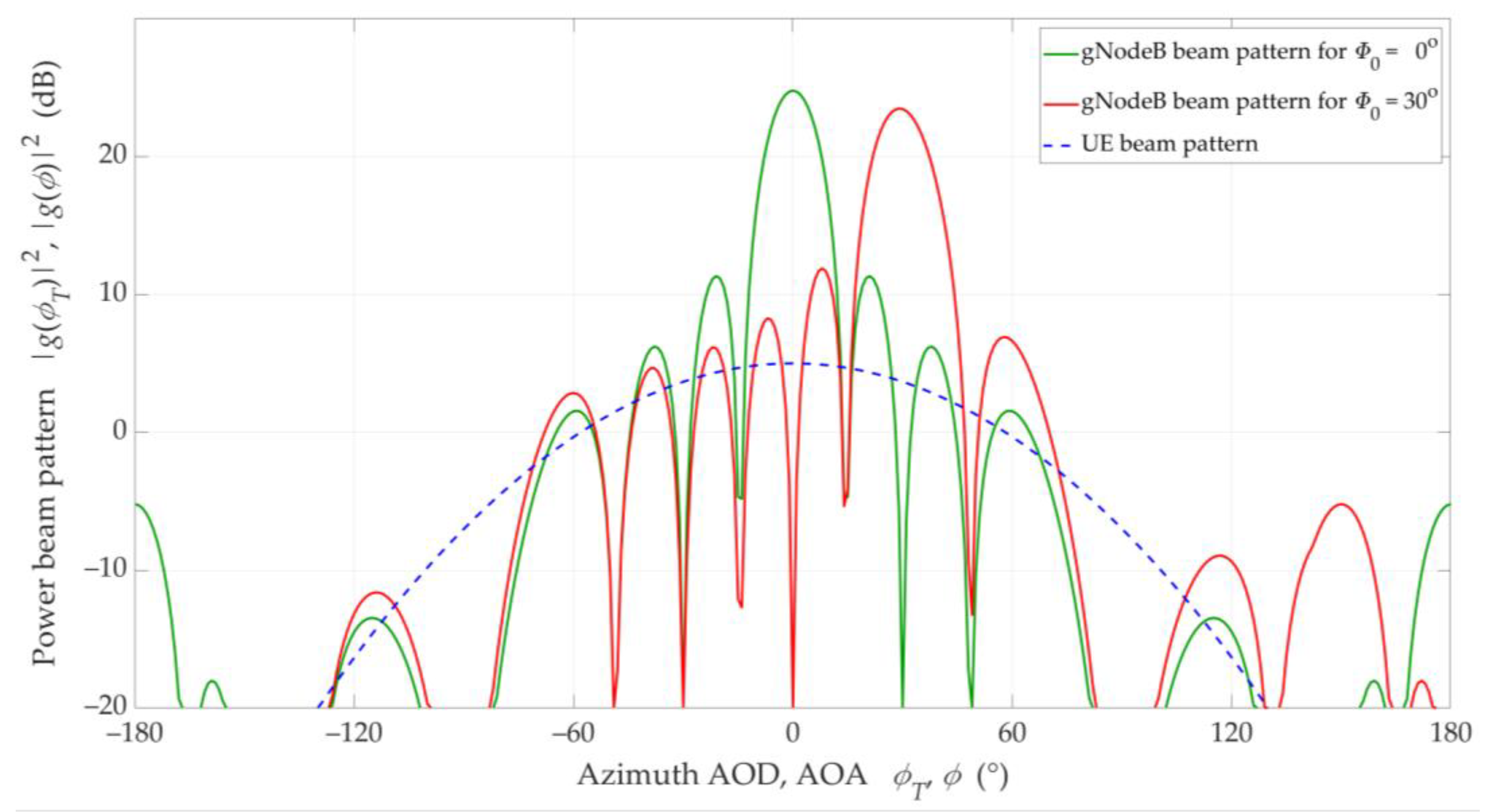
- normalized power patterns , , and , of the serving and interfering transmitting and receiving beams, respectively, where denotes AOD in the elevation and azimuth planes, respectively;
- gains , , and of the serving and interfering transmitting and receiving beams, respectively;
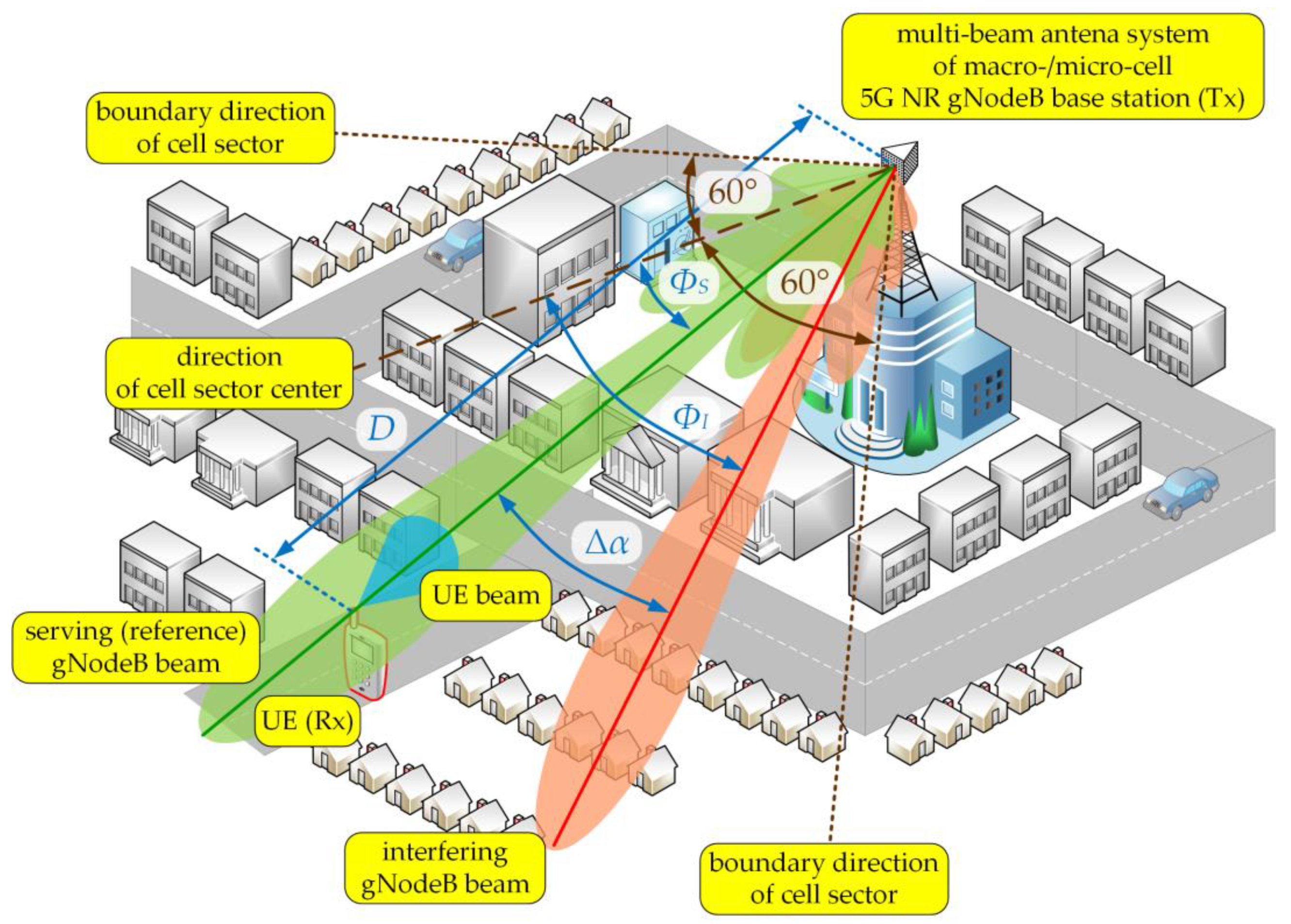
- the Tx-Rx distances, i.e., and between the serving and interfering mobile stations (user equipment, i.e., UE-S and UE-I) and gNodeB for the UL scenario, respectively, or for the DL scenario;
- the type of propagation environment defined by the TDL or PDP and rms delay spread.
- Estimation of consists in the generation of a set of propagation paths departing from the transmitting antennas of the serving and interfering links and their transformation in a system composed of the semi-ellipsoid set. The generation procedure of AODs, uses the properties of the normalized power radiation patterns [36]:
- defining the scenario parameters,
- determining the MPM parameters,
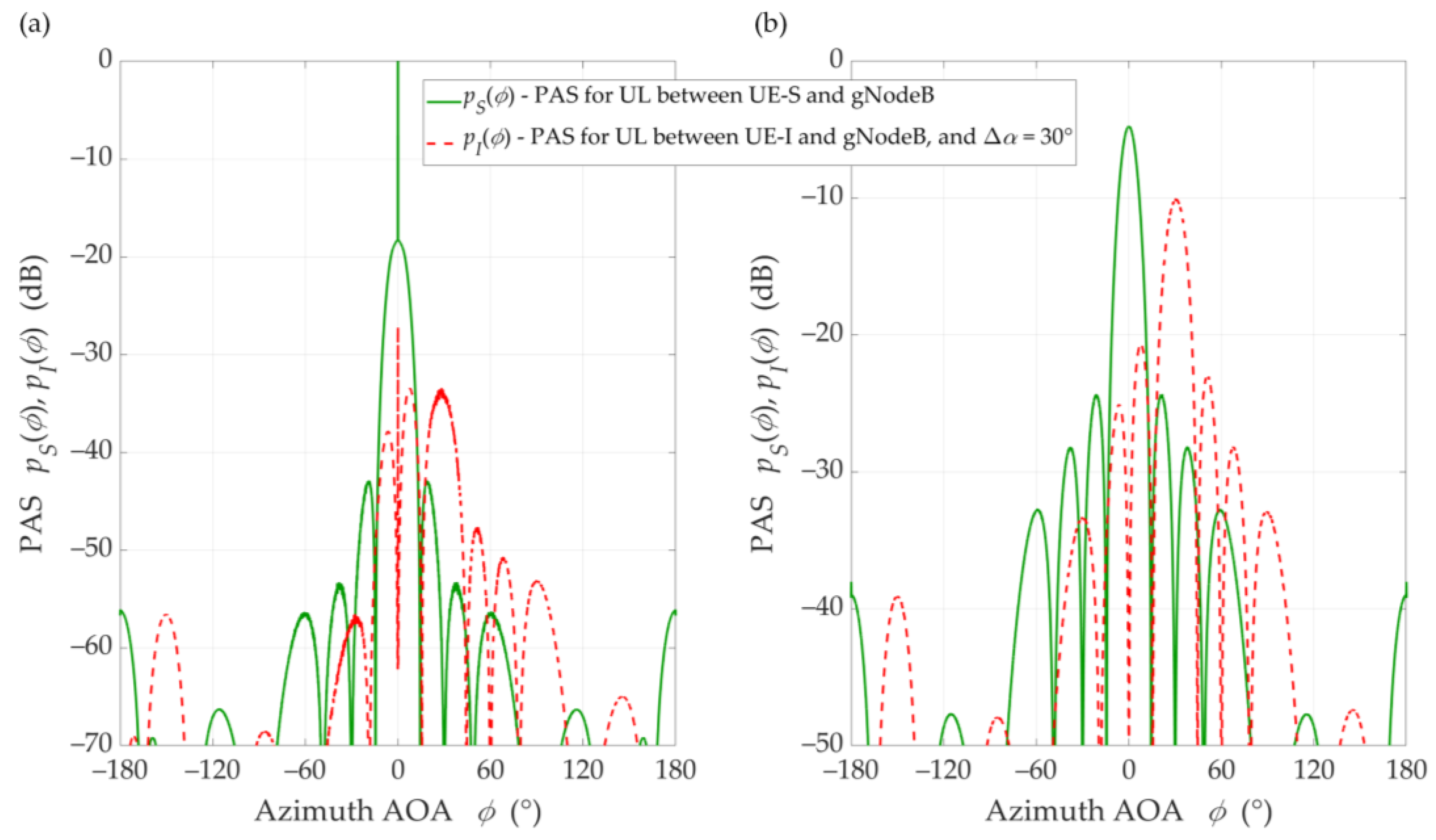
- determining the PASs for the serving and interfering links based on simulation studies,
- calculating the powers for the determined PASs,
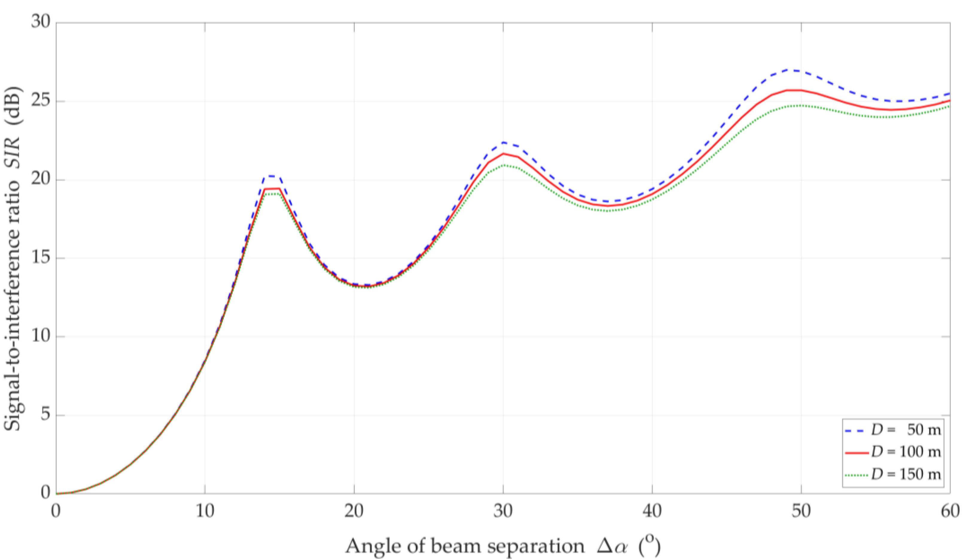
- calculating the SIR finally.
4. Assumptions and Scenarios of Simulation Studies
5. Simulation Results
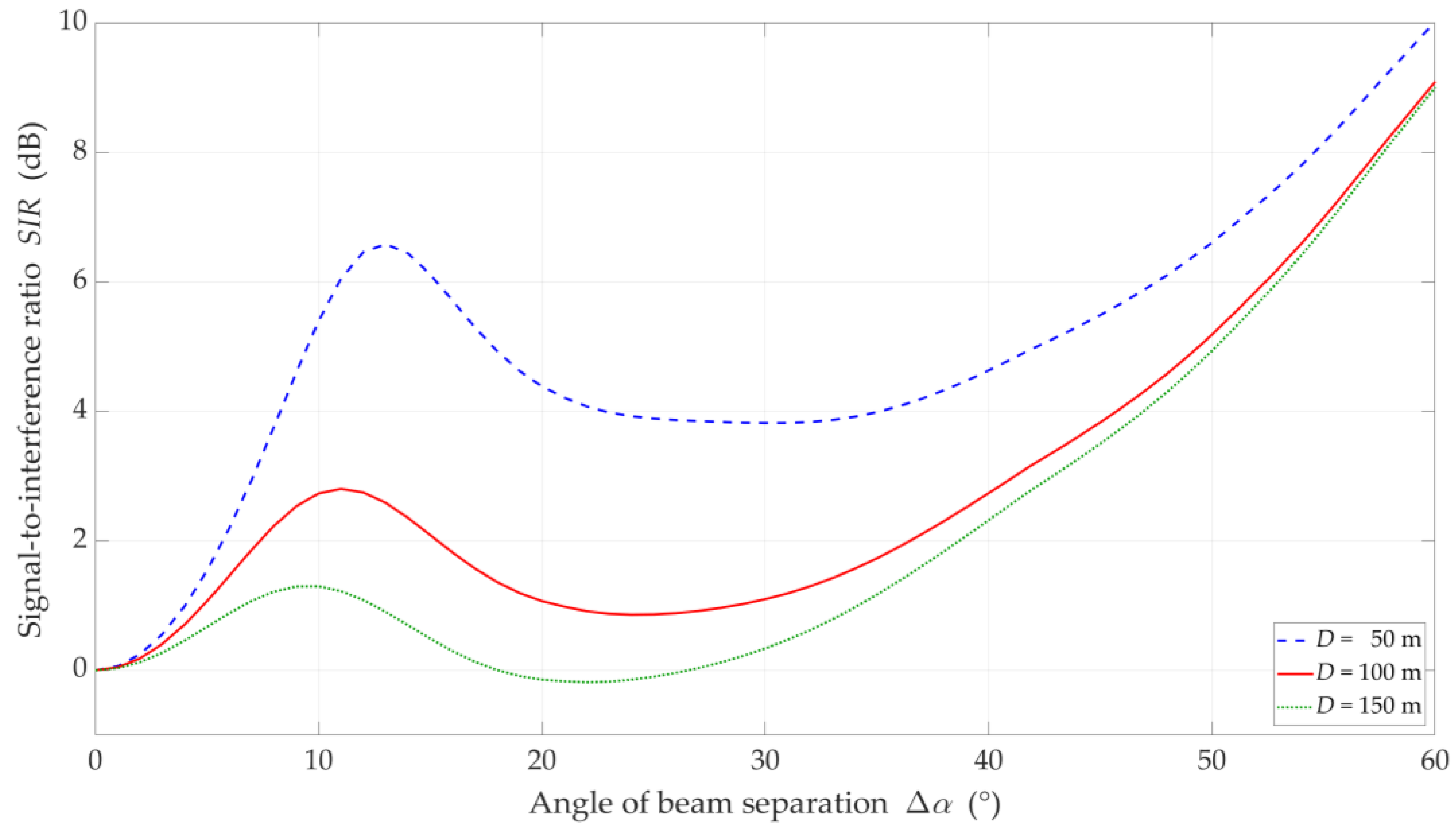
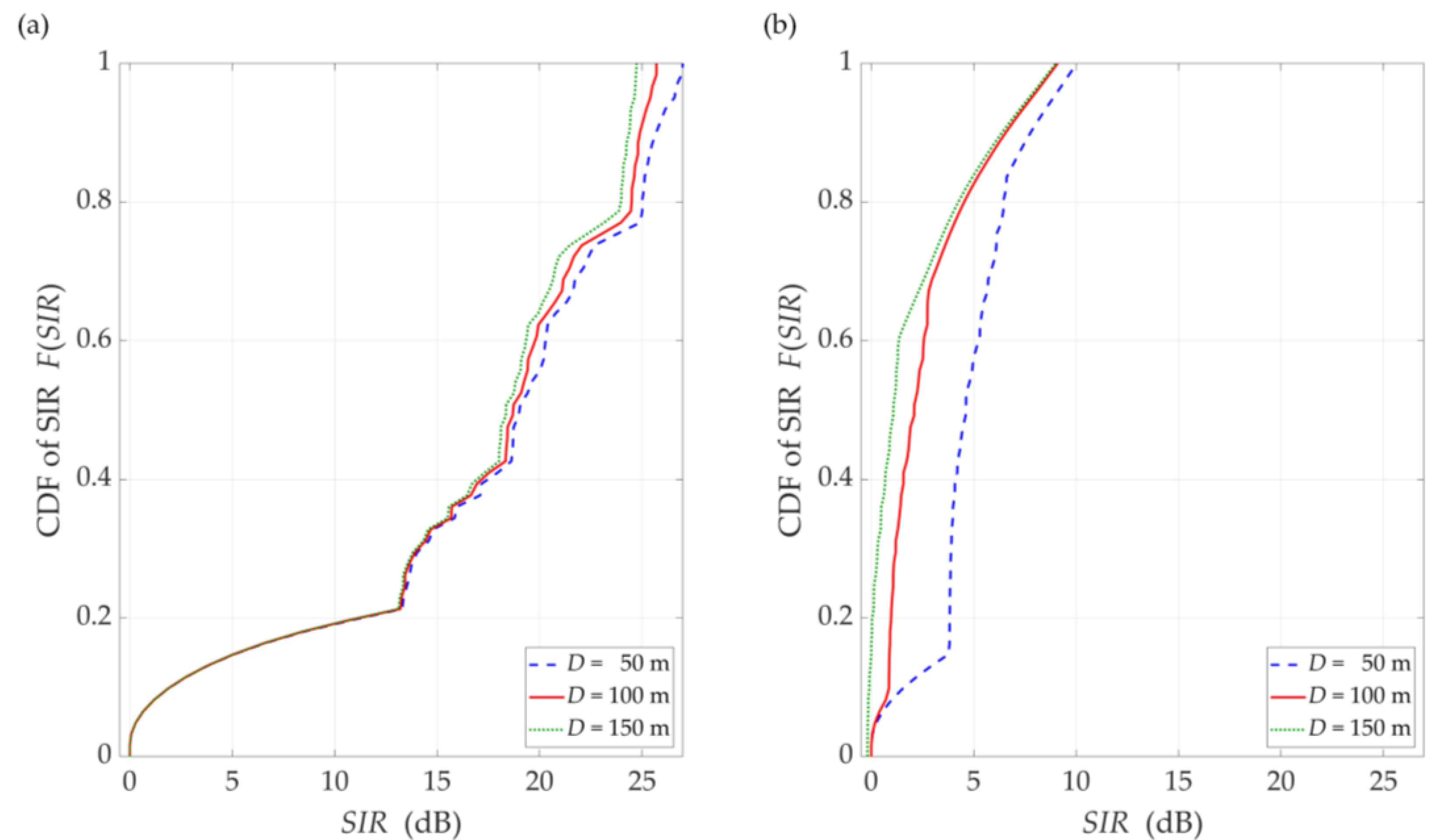
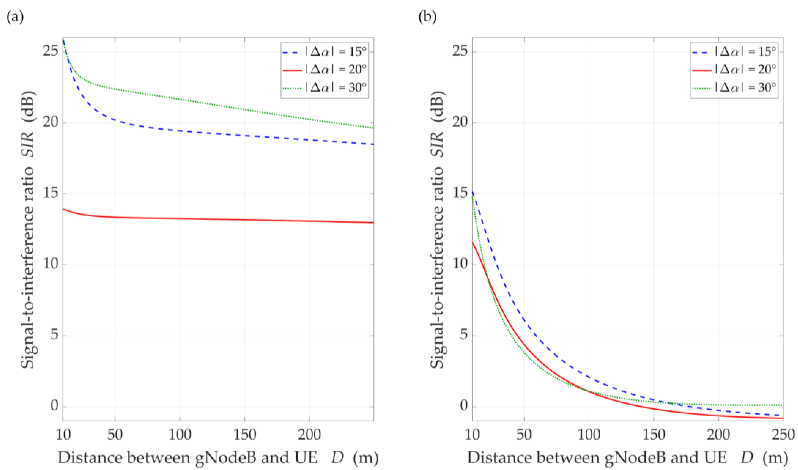
5.1. DL Scenario
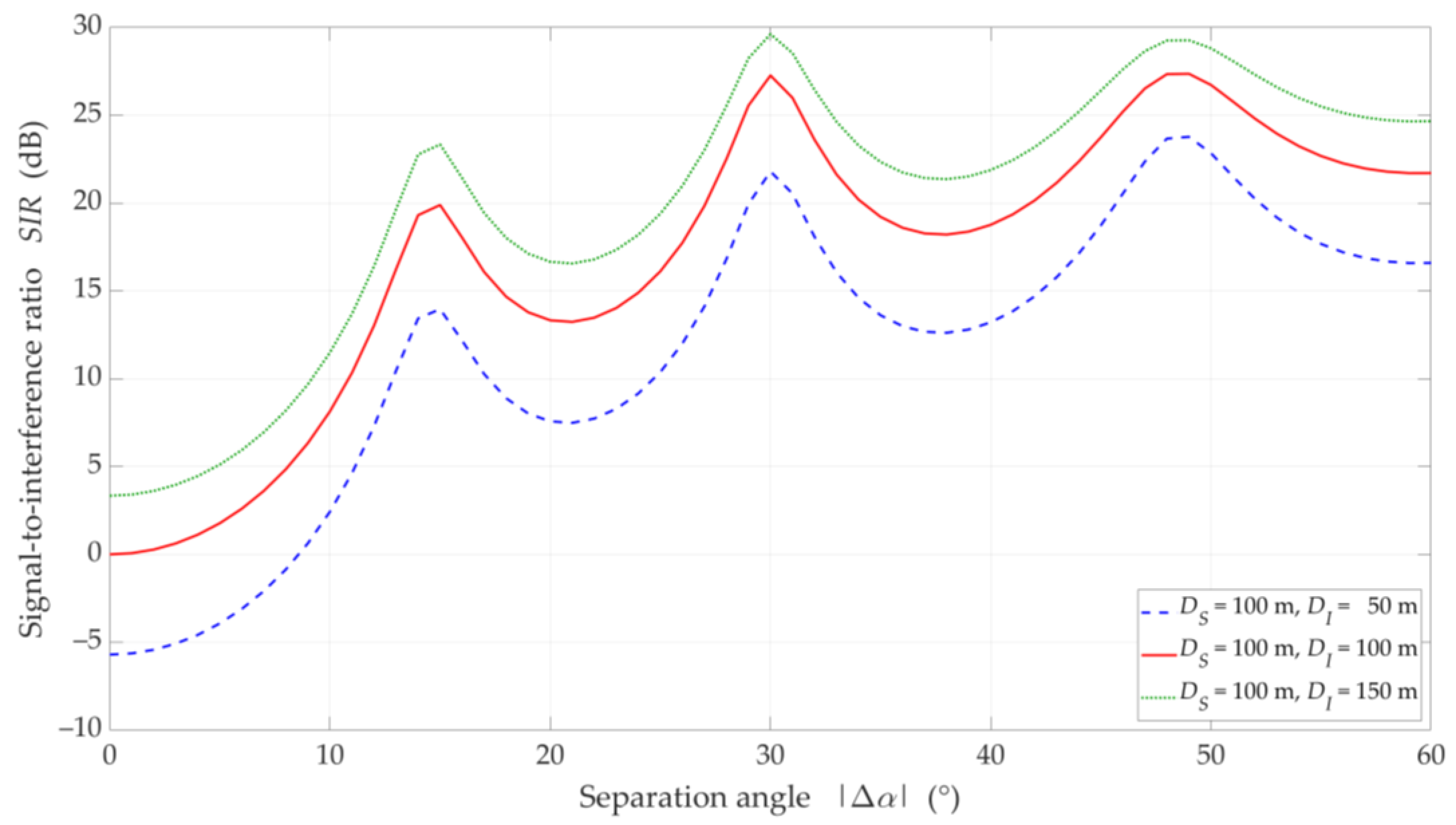
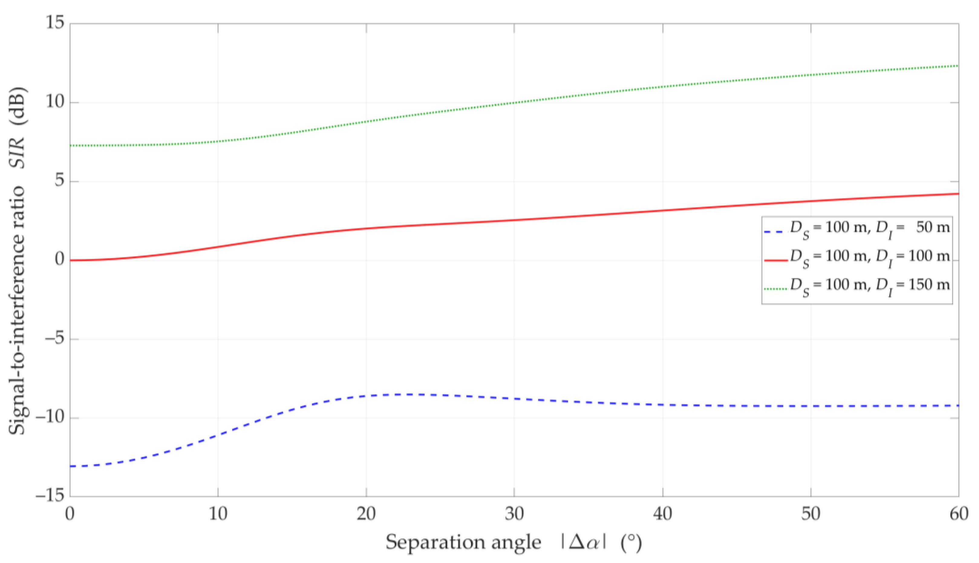
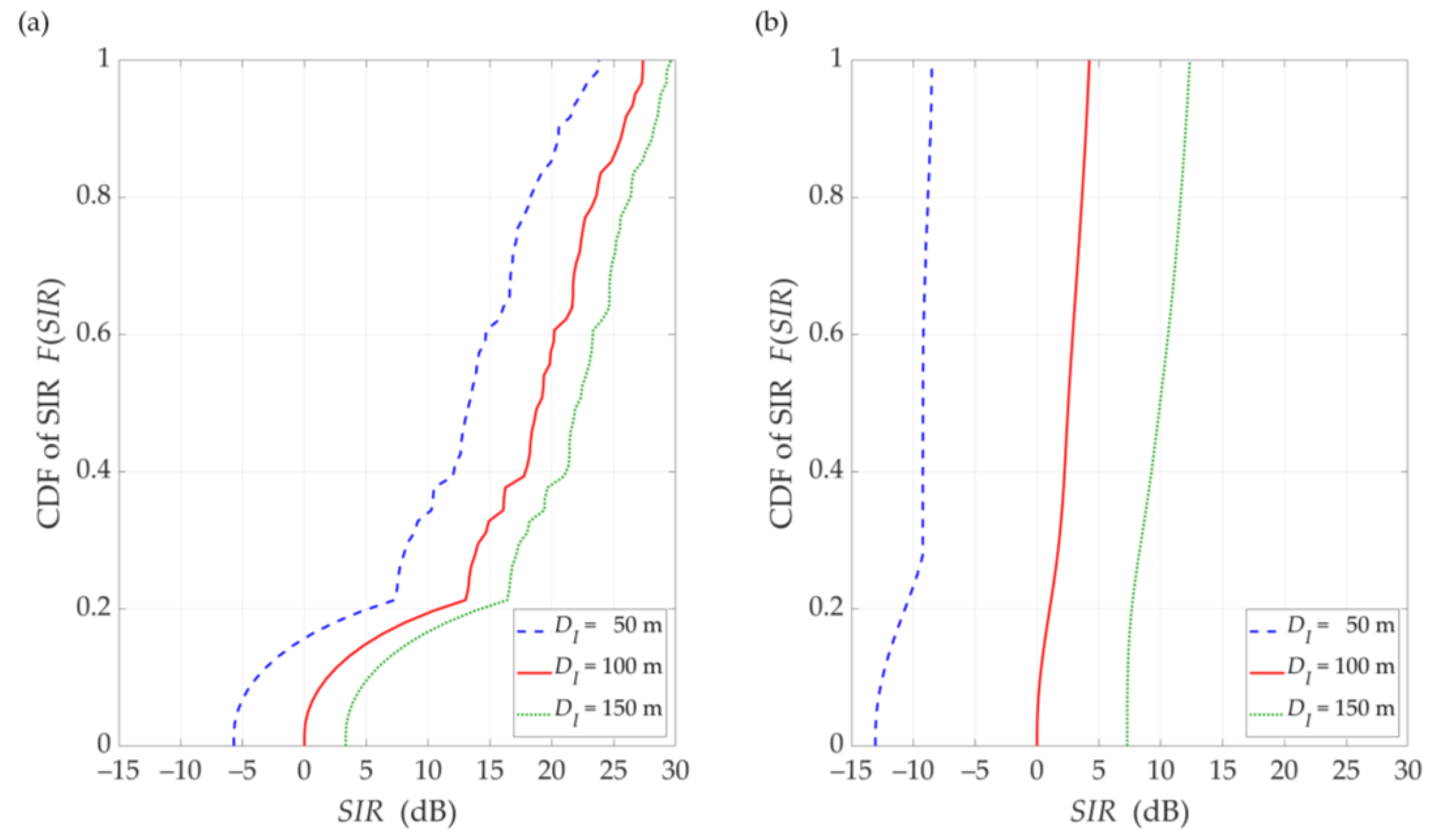
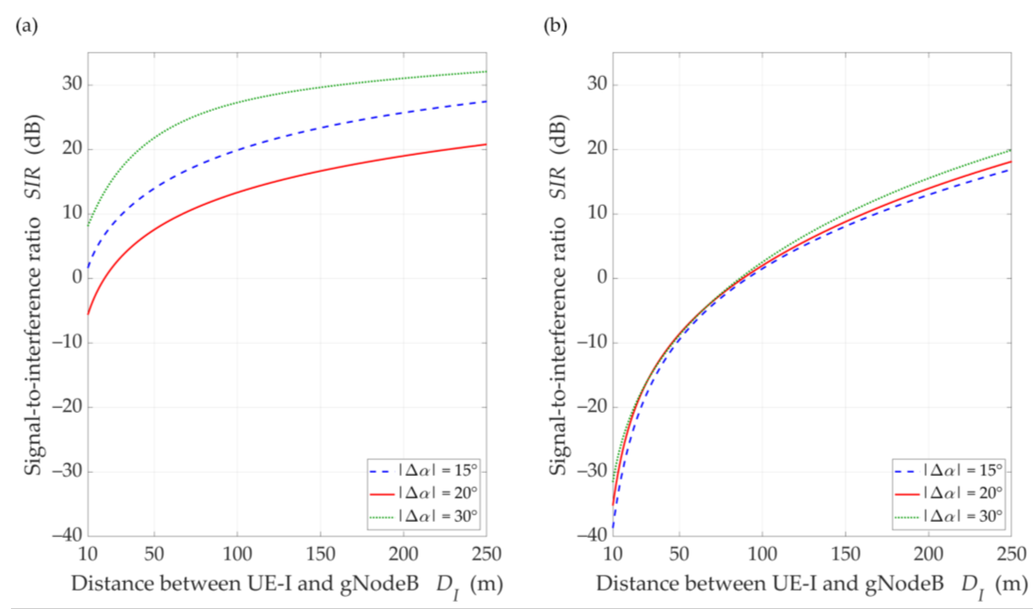
5.2. UL Scenario
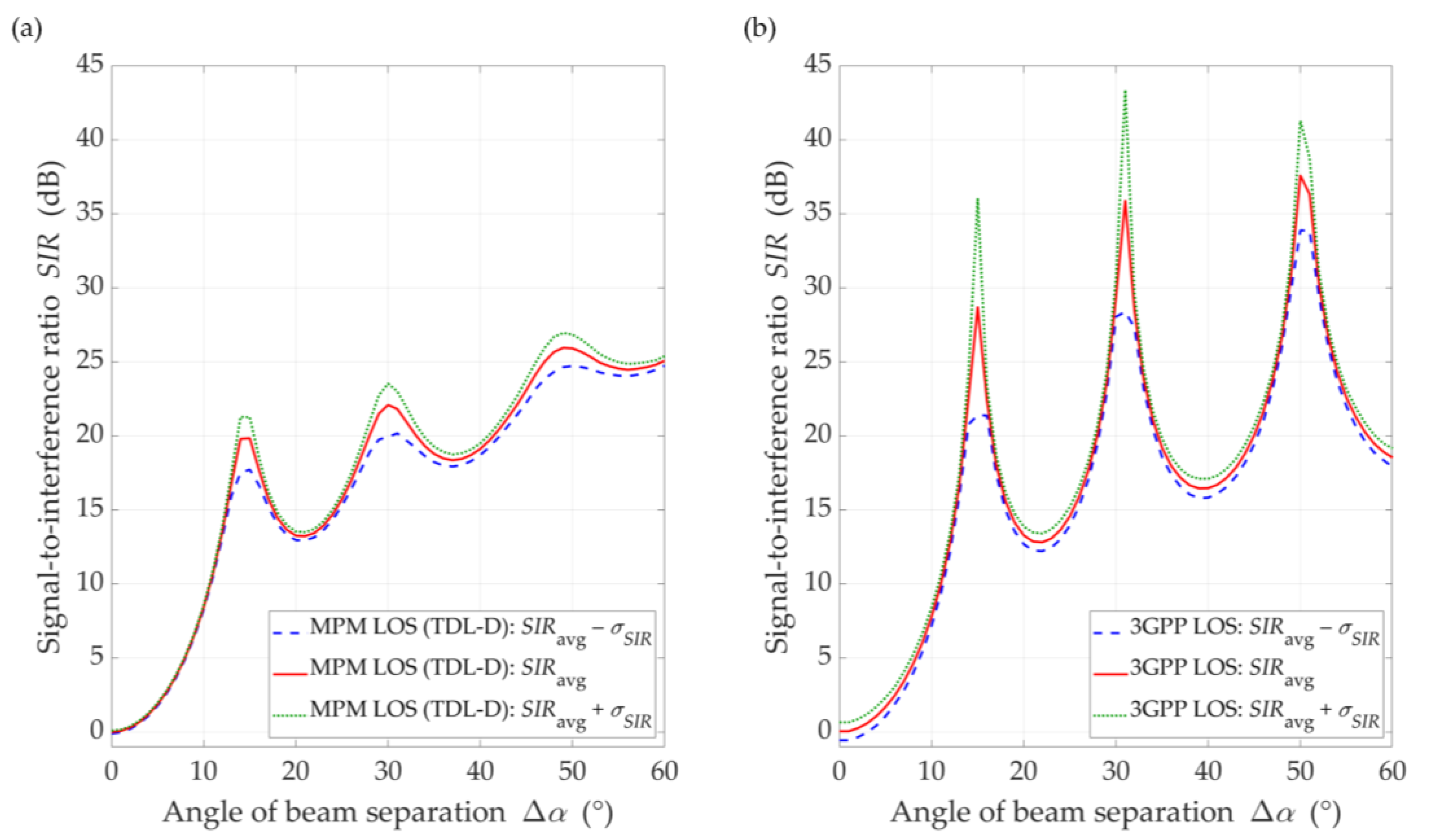
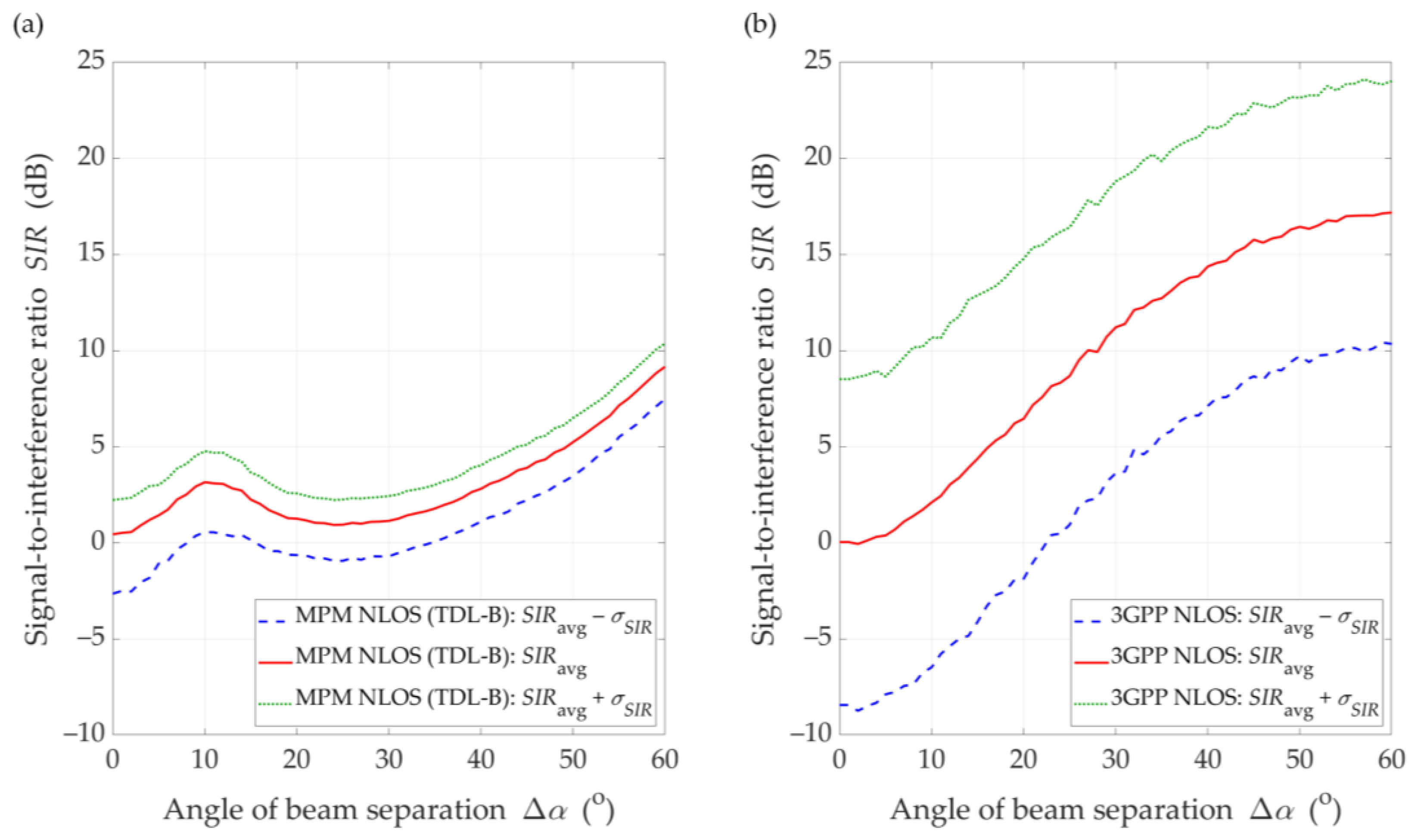
5.3. Exemplary Comparison of MPM with 3GPP Approach for DL Scenario
6. Conclusions
Author Contributions
Funding
Institutional Review Board Statement
Informed Consent Statement
Data Availability Statement
Acknowledgments
Conflicts of Interest
Abbreviations
| 3D | three-dimensional |
| 3GPP | 3rd Generation Partnership Project |
| 5G | fifth-generation |
| AOA | angle of arrival |
| AOD | angle of departure |
| CDF | cumulative distribution function |
| DL | downlink |
| GBM | geometry-based model |
| gNodeB | 5G base station |
| ITU | International Telecommunication Union |
| LOS | line-of-sight |
| MIMO | multiple-input-multiple-output |
| mmWave | millimeter-wave |
| MPM | multi-ellipsoidal propagation model |
| NLOS | non-line-of-sight |
| NR | New Radio |
| PAS | power angular spectrum |
| PDP | power delay profile |
| Rx | receiver |
| SIR | signal-to-interference ratio |
| TDL | tapped delay line |
| Tx | transmitter |
| UE | user equipment |
| UE-I | interfering UE |
| UE-S | serving UE |
| UMa | urban macro |
| UL | uplink |
Symbols
| AOA of individual propagation path | |
| AOD of individual propagation path | |
| normalized power pattern of receiving antenna | |
| normalized power pattern of interfering transmitting antenna | |
| normalized power pattern of serving transmitting antenna | |
| direction of receiving beam | |
| direction of interfering receiving beam | |
| direction of serving receiving beam | |
| direction of transmitting beam | |
| direction of interfering transmitting beam | |
| direction of serving transmitting beam | |
| separation angle between serving and interference beams | |
| path loss correction coefficient (relationship between attenuation of propagation environment for different distances) | |
| angular dispersion of local scattering components in elevation plane | |
| angular dispersion of local scattering components in azimuth plane | |
| elevation AOA of individual propagation path | |
| elevation AOD of individual propagation path | |
| direction of receiving (gNodeB) beam in relation to direction of cell sector center in UL scenario | |
| direction of interfering transmitting (gNodeB) beam in relation to direction of cell sector center in DL scenario | |
| direction of serving transmitting (gNodeB)beam in relation to direction of cell sector center in DL scenario | |
| azimuth AOA of individual propagation path | |
| azimuth AOD of individual propagation path | |
| standard deviation of SIR for confidence interval analysis | |
| standard deviation of SIR for 3GPP model and LOS conditions | |
| standard deviation of SIR for 3GPP model and NLOS conditions | |
| standard deviation of SIR for Model and LOS/NLOS conditions | |
| standard deviation of SIR for MPM and LOS conditions | |
| standard deviation of SIR for MPM and NLOS conditions | |
| delay of nth time-cluster in PDP/TDL | |
| auxiliary variable used to compute | |
| major semi-axis of nth ellipsoid along x-axis | |
| minor semi-axis of nth ellipsoid along y-axis | |
| normalizing constant | |
| lightspeed | |
| minor semi-axis of nth ellipsoid along z-axis | |
| distance between Tx and Rx or between gNodeB (Rx) and UE (Tx) in DL | |
| distance between UE-I (Tx) and gNodeB (Rx) in UL | |
| distance between UE-S (Tx) and gNodeB (Rx) in UL | |
| CDF of SIR | |
| distribution of path power | |
| 2D von Mises distribution describing local scattering components | |
| distribution of AOD for interfering link | |
| distribution of AOD for serving link | |
| gain of receiving beam | |
| gain of interfering transmitting beam | |
| gain of serving transmitting beam | |
| zero-order modified Bessel function of imaginary argument | |
| number of all time-clusters in analyzed PDP/TDL | |
| number of analyzed time-cluster in PDP/TDL | |
| power of interfering signal | |
| power of serving signal | |
| path loss | |
| path loss for wireless links between UE-I and gNodeB at distance | |
| path loss for wireless links between UE-S and gNodeB at distance | |
| power of individual propagation path | |
| mean power of nth time-cluster in PDP/TDL (nth local extreme of PDP/TDL) | |
| PAS seen at the output of receiving antenna for interfering link | |
| PAS seen at the output of receiving antenna for serving link | |
| PAS in vicinity of receiving antenna for interfering link | |
| PAS in vicinity of receiving antenna for serving link | |
| radial coordinate in spherical system with origin in Tx | |
| SIR | |
| average SIR for confidence interval analysis | |
| confidence intervals of SIR |
References
- Gupta, A.; Jha, R.K. A Survey of 5G network: Architecture and emerging technologies. IEEE Access 2015, 3, 1206–1232. [Google Scholar] [CrossRef]
- Agiwal, M.; Roy, A.; Saxena, N. Next generation 5G wireless networks: A comprehensive survey. IEEE Commun. Surv. Tutor. 2016, 18, 1617–1655. [Google Scholar] [CrossRef]
- Araújo, D.C.; Maksymyuk, T.; de Almeida, A.L.; Maciel, T.; Mota, J.C.; Jo, M. Massive MIMO: Survey and future research topics. IET Commun. 2016, 10, 1938–1946. [Google Scholar] [CrossRef]
- Busari, S.A.; Huq, K.M.S.; Mumtaz, S.; Dai, L.; Rodriguez, J. Millimeter-wave massive MIMO communication for future wireless systems: A survey. IEEE Commun. Surv. Tutor. 2018, 20, 836–869. [Google Scholar] [CrossRef]
- Yacoub, M.D. Fading distributions and co-channel interference in wireless systems. IEEE Antennas Propag. Mag. 2000, 42, 150–160. [Google Scholar] [CrossRef]
- Rui, X.; Jin, R.; Geng, J. Performance analysis of MIMO MRC systems in the presence of self-interference and co-channel interferences. IEEE Signal Process. Lett. 2007, 14, 801–803. [Google Scholar] [CrossRef]
- Fernandes, F.; Ashikhmin, A.; Marzetta, T.L. Inter-cell interference in noncooperative TDD large scale antenna systems. IEEE J. Sel. Areas Commun. 2013, 31, 192–201. [Google Scholar] [CrossRef]
- Guidolin, F.; Nekovee, M. Investigating spectrum sharing between 5G millimeter wave networks and fixed satellite systems. In Proceedings of the 2015 IEEE Globecom Workshops (GC Wkshps), San Diego, CA, USA, 6–10 December 2015; pp. 1–7. [Google Scholar] [CrossRef]
- Kim, S.; Visotsky, E.; Moorut, P.; Bechta, K.; Ghosh, A.; Dietrich, C. Coexistence of 5G with the incumbents in the 28 and 70 GHz bands. IEEE J. Sel. Areas Commun. 2017, 35, 1254–1268. [Google Scholar] [CrossRef]
- Hattab, G.; Visotsky, E.; Cudak, M.; Ghosh, A. Toward the Coexistence of 5G Mmwave Networks with Incumbent Systems beyond 70 GHz. IEEE Wirel. Commun. 2018, 25, 18–24. [Google Scholar] [CrossRef]
- Cho, Y.; Kim, H.-K.; Nekovee, M.; Jo, H.-S. Coexistence of 5G with satellite services in the millimeter-wave band. IEEE Access 2020, 8, 163618–163636. [Google Scholar] [CrossRef]
- Kim, T.; Park, S. Statistical Beamforming for massive MIMO systems with distinct spatial correlations. Sensors 2020, 20, 6255. [Google Scholar] [CrossRef] [PubMed]
- Arshad, J.; Rehman, A.; Rehman, A.U.; Ullah, R.; Hwang, S.O. Spectral efficiency augmentation in uplink massive MIMO systems by increasing transmit power and uniform linear array gain. Sensors 2020, 20, 4982. [Google Scholar] [CrossRef] [PubMed]
- 3GPP. Study on Channel Model for Frequencies from 0.5 to 100 GHz; 3rd Generation Partnership Project (3GPP), Technical Specification Group Radio Access Network: Valbonne, France, 2019. [Google Scholar]
- Kilzi, A.; Farah, J.; Nour, C.A.; Douillard, C. Mutual successive interference cancellation strategies in NOMA for enhancing the spectral efficiency of CoMP systems. IEEE Trans. Commun. 2020, 68, 1213–1226. [Google Scholar] [CrossRef]
- Hassan, N.; Fernando, X. Interference mitigation and dynamic user association for load balancing in heterogeneous networks. IEEE Trans. Veh. Technol. 2019, 68, 7578–7592. [Google Scholar] [CrossRef]
- Ali, K.S.; Elsawy, H.; Chaaban, A.; Alouini, M. Non-orthogonal multiple access for large-scale 5G networks: Interference aware design. IEEE Access 2017, 5, 21204–21216. [Google Scholar] [CrossRef]
- Mahmood, N.H.; Pedersen, K.I.; Mogensen, P. Interference aware inter-cell rank coordination for 5G systems. IEEE Access 2017, 5, 2339–2350. [Google Scholar] [CrossRef]
- Elgendi, H.; Mäenpää, M.; Levanen, T.; Ihalainen, T.; Nielsen, S.; Valkama, M. Interference measurement methods in 5G NR: Principles and performance. In Proceedings of the IEEE 16th International Symposium on Wireless Communication Systems (ISWCS), Oulu, Finland, 27–30 August 2019; pp. 233–238. [Google Scholar] [CrossRef]
- Wang, H.; Khilkevich, V.; Zhang, Y.; Fan, J. Estimating radio-frequency interference to an antenna due to near-field coupling using decomposition method based on reciprocity. IEEE Trans. Electromagn. Compat. 2013, 55, 1125–1131. [Google Scholar] [CrossRef]
- Fan, J. Near-field scanning for EM emission characterization. IEEE Electromagn. Compat. Mag. 2015, 4, 67–73. [Google Scholar] [CrossRef]
- Liu, E.; Zhao, W.; Wang, B.; Gao, S.; Wei, X. Near-field scanning and its EMC applications. In Proceedings of the IEEE International Symposium on Electromagnetic Compatibility Signal/Power Integrity (EMCSI), Washington, DC, USA, 7–11 August 2017; pp. 327–332. [Google Scholar] [CrossRef]
- Shu, Y.; Wei, X.; Yang, Y. Patch antenna radiation pattern evaluation based on phaseless and single-plane near-field scanning. In Proceedings of the IEEE International Conference on Computational Electromagnetics (ICCEM), Shanghai, China, 20–22 March 2019; pp. 1–3. [Google Scholar] [CrossRef]
- Zhao, Y.; Baharuddin, M.H.; Smartt, C.; Zhao, X.; Yan, L.; Liu, C.; Thomas, D.W.P. Measurement of near-field electromagnetic emissions and characterization based on equivalent dipole model in time-domain. IEEE Trans. Electromagn. Compat. 2020, 62, 1237–1246. [Google Scholar] [CrossRef]
- Xue, Q.; Li, B.; Zuo, X.; Yan, Z.; Yang, M. Cell Capacity for 5G Cellular Network with Inter-Beam Interference. In Proceedings of the IEEE International Conference on Signal Processing, Communications and Computing (ICSPCC), Hong Kong, China, 5–8 August 2016; pp. 1–5. [Google Scholar] [CrossRef]
- Elsayed, M.; Shimotakahara, K.; Erol-Kantarci, M. Machine Learning-based inter-beam inter-cell interference mitigation in mmWave. In Proceedings of the IEEE International Conference on Communications (ICC), Dublin, Ireland, 7–11 June 2020; pp. 1–6. [Google Scholar] [CrossRef]
- Lee, H.; Park, Y.; Hong, D. Resource Split Full duplex to mitigate inter-cell interference in ultra-dense small cell networks. IEEE Access 2018, 6, 37653–37664. [Google Scholar] [CrossRef]
- Xu, S.; Li, Y.; Gao, Y.; Liu, Y.; Gačanin, H. Opportunistic coexistence of LTE and WiFi for future 5G system: Experimental performance evaluation and analysis. IEEE Access 2018, 6, 8725–8741. [Google Scholar] [CrossRef]
- Ziółkowski, C.; Kelner, J.M. Antenna pattern in three-dimensional modelling of the arrival angle in simulation studies of wireless channels. IET Microw. Antennas Propag. 2017, 11, 898–906. [Google Scholar] [CrossRef]
- Ziółkowski, C.; Kelner, J.M. Statistical evaluation of the azimuth and elevation angles seen at the output of the receiving antenna. IEEE Trans. Antennas Propag. 2018, 66, 2165–2169. [Google Scholar] [CrossRef]
- Kelner, J.M.; Ziółkowski, C. Multi-elliptical geometry of scatterers in modeling propagation effect at receiver. In Antennas and Wave Propagation; Pinho, P., Ed.; IntechOpen: London, UK, 2018; pp. 115–141. ISBN 978-953-51-6014-4. [Google Scholar] [CrossRef]
- Bechta, K.; Ziółkowski, C.; Kelner, J.M.; Nowosielski, L. Downlink interference in multi-beam 5G macro-cell. In Proceedings of the IEEE 23rd International Microwave and Radar Conference (MIKON), Warsaw, Poland, 5–8 October 2020; pp. 140–143. [Google Scholar] [CrossRef]
- Parsons, J.D.; Bajwa, A.S. Wideband characterisation of fading mobile radio channels. IEE Proc. F Commun. Radar Signal Process. 1982, 129, 95–101. [Google Scholar] [CrossRef]
- Ziółkowski, C.; Kelner, J.M. Estimation of the reception angle distribution based on the power delay spectrum or profile. Int. J. Antennas Propag. 2015, 2015, e936406. [Google Scholar] [CrossRef]
- Abdi, A.; Barger, J.A.; Kaveh, M. A parametric model for the distribution of the angle of arrival and the associated correlation function and power spectrum at the mobile station. IEEE Trans. Veh. Technol. 2002, 51, 425–434. [Google Scholar] [CrossRef]
- Vaughan, R.; Bach Andersen, J. Channels, Propagation and Antennas for Mobile Communications; IET Electromagnetic Waves Series; Institution of Engineering and Technology: London, UK, 2003; ISBN 978-0-86341-254-7. [Google Scholar]
- Rappaport, T.S.; MacCartney, G.R.; Samimi, M.K.; Sun, S. Wideband millimeter-wave propagation measurements and channel models for future wireless communication system design. IEEE Trans. Commun. 2015, 63, 3029–3056. [Google Scholar] [CrossRef]
- ITU. Recommendation ITU-R P.837-7: Characteristics of Precipitation for Propagation Modelling; P Series Radiowave Propagation; International Telecommunication Union (ITU): Geneva, Switzerland, 2017. [Google Scholar]
- ITU. Recommendation ITU-R P.838-3: Specific Attenuation Model for Rain for Use in Prediction Methods; P Series Radiowave Propagation; International Telecommunication Union (ITU): Geneva, Switzerland, 2005. [Google Scholar]
- Han, C.; Duan, S. Impact of atmospheric parameters on the propagated signal power of millimeter-wave bands based on real measurement data. IEEE Access 2019, 7, 113626–113641. [Google Scholar] [CrossRef]
- Huang, J.; Cao, Y.; Raimundo, X.; Cheema, A.; Salous, S. Rain statistics investigation and rain attenuation modeling for millimeter wave short-range fixed links. IEEE Access 2019, 7, 156110–156120. [Google Scholar] [CrossRef]
- 3GPP. Evolved Universal Terrestrial Radio Access (E-UTRA) and Universal Terrestrial Radio Access (UTRA); Radio Frequency (RF) Requirement Background for Active Antenna System (AAS) Base Station (BS); 3rd Generation Partnership Project (3GPP): Valbonne, France, 2019. [Google Scholar]
- Kelner, J.M.; Ziółkowski, C. Interference in multi-beam antenna system of 5G network. Int. J. Electron. Telecommun. 2020, 66, 17–23. [Google Scholar] [CrossRef]
- Bechta, K.; Du, J.; Rybakowski, M. Rework the radio link budget for 5G and beyond. IEEE Access 2020, 8, 211585–211594. [Google Scholar] [CrossRef]
- Almesaeed, R.; Ameen, A.S.; Mellios, E.; Doufexi, A.; Nix, A.R. A proposed 3D extension to the 3GPP/ITU channel model for 800 MHz and 2.6 GHz bands. In Proceedings of the IEEE 8th European Conference on Antennas and Propagation (EuCAP). Hague, The Netherlands, 6–11 April 2014; pp. 3039–3043. [Google Scholar] [CrossRef]
- Ademaj, F.; Taranetz, M.; Rupp, M. 3GPP 3D MIMO Channel Model: A Holistic Implementation Guideline for Open Source Simulation Tools. EURASIP J. Wirel. Commun. Netw. 2016, 2016, 55. [Google Scholar] [CrossRef]
- Rappaport, T.S.; Sun, S.; Shafi, M. Investigation and Comparison of 3GPP and NYUSIM Channel Models for 5G Wireless Communications. In Proceedings of the IEEE 86th Vehicular Technology Conference (VTC-Fall), Toronto, ON, Canada, 24–27 September 2017; pp. 1–5. [Google Scholar] [CrossRef]
- Sheikh, M.U.; Jäntti, R.; Hämäläinen, J. Performance Comparison of Ray Tracing and 3GPP Street Canyon Model in Microcellular Environment. In Proceedings of the IEEE 27th International Conference on Telecommunications (ICT), Bali, Indonesia, 5–7 October 2020; pp. 1–5. [Google Scholar] [CrossRef]
- Bechta, K.; Ziółkowski, C.; Kelner, J.M.; Nowosielski, L. Modeling of downlink interference in massive MIMO 5G macro-cell. Sensors 2021, 21, 597. [Google Scholar] [CrossRef] [PubMed]


Publisher’s Note: MDPI stays neutral with regard to jurisdictional claims in published maps and institutional affiliations. |
© 2021 by the authors. Licensee MDPI, Basel, Switzerland. This article is an open access article distributed under the terms and conditions of the Creative Commons Attribution (CC BY) license (http://creativecommons.org/licenses/by/4.0/).
Share and Cite
Bechta, K.; Kelner, J.M.; Ziółkowski, C.; Nowosielski, L. Inter-Beam Co-Channel Downlink and Uplink Interference for 5G New Radio in mm-Wave Bands. Sensors 2021, 21, 793. https://doi.org/10.3390/s21030793
Bechta K, Kelner JM, Ziółkowski C, Nowosielski L. Inter-Beam Co-Channel Downlink and Uplink Interference for 5G New Radio in mm-Wave Bands. Sensors. 2021; 21(3):793. https://doi.org/10.3390/s21030793
Chicago/Turabian StyleBechta, Kamil, Jan M. Kelner, Cezary Ziółkowski, and Leszek Nowosielski. 2021. "Inter-Beam Co-Channel Downlink and Uplink Interference for 5G New Radio in mm-Wave Bands" Sensors 21, no. 3: 793. https://doi.org/10.3390/s21030793
APA StyleBechta, K., Kelner, J. M., Ziółkowski, C., & Nowosielski, L. (2021). Inter-Beam Co-Channel Downlink and Uplink Interference for 5G New Radio in mm-Wave Bands. Sensors, 21(3), 793. https://doi.org/10.3390/s21030793