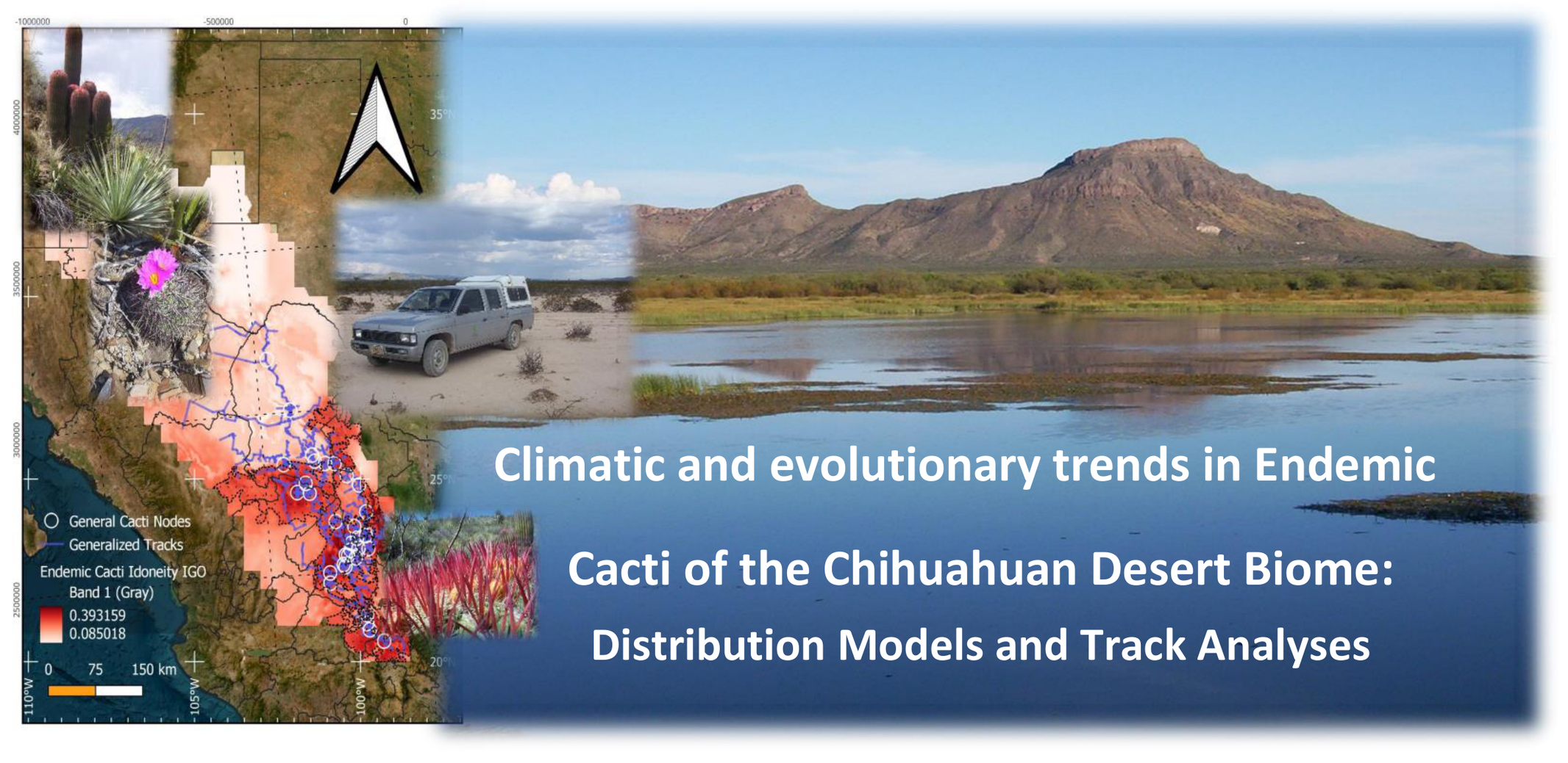
Climatic and Evolutionary Trends in Endemic Cacti of the Chihuahuan Desert Biome: Distribution Models and Track Analyses

Abstract

The Chihuahuan Desert Biome (CDB), the largest semi-arid region in North America, has undergone repeated climatic fluctuations during the Interglacial–Glacial Oscillation (IGO) of the last eight million years. We investigated biogeographic and evolutionary patterns of endemic cacti within the present-day Interglacial and the Last Glacial by examining 119 strict endemics, including 75 suitable for Species Distribution Modeling (SDM) and 44 microareal strict endemics, together representing 36.17% of the 329 species in the biome. Cacti probably originated in South America after substantial separation from Africa, with pollen fossils documenting their presence in Mexico by 51.6 Ma. Climatic reconstructions for each phase were developed using regional numerical and co-kriging methods following Sánchez-Santillán and García, complemented by paleoclimatic evidence from Scotese, Roy-Priyadarsi, Van Devender, and Betancourt. MAXENT SDMs and PANBIOTRACKS’ track-node analyses were applied to 3719 specimens representing 2015 localities to explore the colonization patterns and broad evolutionary trends. Combined suitability layers and panbiogeographic analyses revealed a predominant southeastern-to-northwestern colonization pattern, largely following the western flank of the Sierra Madre Oriental and intermontane valleys. The northern sectors were less diverse, more arid, and apparently colonized more recently, whereas the southern sectors concentrated much of the endemic richness and connectivity. The concordance among climatic suitability patterns, tracks, nodes, and the available phylogenetic evidence supports a major role of climatic oscillations in shaping the spatial and evolutionary history of endemic cacti throughout the CDB.

1. Introduction

The Chihuahuan Desert Biome (CDB) is a major ecosystem assemblage fluctuating between the Interglacial (IG) and Glacial (G) phases in a present-day Glaciation Era [1,2,3], established primarily over the last 8 Ma after the gradual closure of the Central American oceanic bridge [1,4,5]. The continent experienced significant climate changes due to alterations in warm oceanic currents, slowing the influx of cold waters from the Antarctic into the Caribbean Sea [1,5]. This happened after regional orogenies and after new seafloors were created by expansionary tectonics, where the hydrosphere can be further held [6,7], highly correlated with important geological proxies [8,9,10] and paleomagnetic evidence [6]. Previously, large orogenies developed in the region, as in the Laramidian (84–43 Ma) [11], and partial correlations with uplifted parts of the Central American Archipelago and other mountains, which also contributed to Laramidia drainage [1,3,5]. A significant climatic process was the increase in humidity toward the equator and the northward shift of arid and semiarid bands, establishing mid–latitude arid regions [5]. Few studies have explored reconstructions of present and past climates in the CDB [8,9], and none have covered track analyses for its cacti. Here, colonization patterns are explored alongside the best-resolved phylogenies. These complementary lines of evidence provide information at different temporal scales and allow recent climatic patterns associated with the IGO to be interpreted within a broader evolutionary and biogeographic framework. Most climatologists accept that we live in an Ice Age [2,3,5], fed by atmospheric dilution and Milankovitch cycles. The iteration, which we call IGO (Glacial–Interglacial Oscillation), has seen 87 cycles since some 8 Ma, and creates climate changes that, in combination with soil use and grazing, are among the drivers of cacti diversity, distribution, and evolution in the CDB [1,12,13]. Cactaceae is a sui generis family containing over 1470 species, with at least 800 occurring in Mexico and the Southern USA [13]. The CDB holds 329 species, with 69.91% (230) being endemic and 119 being strict endemics (36.17%) [14,15,16,17]. Fossil pollen in Central Mexico dates to 16–51.6 Ma [18], with animals as the likely agents of their arrival, probably from South America ([19] and Appendix A.1). Since then, they moved north and west and reached the CDB some 16–20 Ma, after the rise of the Sierra Madre Oriental (SMO; 38–23 Ma to present) [11], which completed the rain shadow from Atlantic sources [8,9,10]. We developed our Species Distribution Models (SDMs) using MAXENT algorithms for the IGO and studied 75 modelable species that occur strictly inside the biome and have sufficient localities, area coverage, or enough separation between groups of sites. Extremely clogged species resembling a single locality, or species with fewer than four sites, were not modeled but were used for richness and general perspectives. The IG model came from the application of Sánchez–Santillán and García methods [20,21], while Scotese’s works [22], particular proxies from Roy–Priyadarsi [8,9,10], and clues from packrat middens [23,24,25,26] were used for selection of climatic influence zones and G modeling. The effects of megafauna and human activities on cacti in the biome have been largely lost to history and may be impossible to reconstruct from the available evidence. Track analyses encompass the calculation of Croizat-inspired patterns that represent ancient biotas, involving evolutionary processes in space, time, and form [27]. Those patterns comprise the graphical integration of biodiversity into identifiable lines and points, tracks and nodes that show estimated patterns of evolution, which were later compared with Halffter’s Cenocrons [28,29]. These explorations include the cladistic content of biology per region and were incorporated into clear methodologies that improved tests by incorporating mathematical and digital algorithms [30], like those we use in this study [31]. We anticipate that the SDMs will highlight areas with the highest suitability for particular species within the phases of the IGO, revealing potential changes in direction, area drift, size, or areal change. We also suggest that they will reveal the general colonization patterns and will moderately fit with the track and node analyses.

1.1. Objectives

The objective was to deepen the understanding of biogeographic-evolutionary patterns of strict-endemic cacti to contribute to the general knowledge of their evolution in space, form, and time, modeling SDMs for the IGO, exploring the ancient biotas through track and node analyses, and using their overlaps to highlight colonization patterns and find potential for dispersal-vicariance trends. Use those elements to test the proposed entrance from the SE portion and its overlap with climatic trends into a northern, arid, less diverse portion and a southern, less arid, highly diverse portion.

1.2. Study Area

The Chihuahuan Desert Biome comprises numerous ecosystems, ranging from extreme arid zones to subhumid montane pine and fir forests [22,25,26] alternating in the IGO. Its geological origin stems from regional compressions and distensions [11], the closure of the Central American seaway [1,4,5], and planetary expansionary processes [6,7]. It is part of the North American Tectonic Plate and was covered by deep waters for most of its history before the water moved into new oceanic basins [6]. Reef evidence points to ancient coastal environments, indicating the gradual drainage and uplift of the region some 75–30 Ma [7]. The movement of the Laramidian sea is closely related to the Laramidian orogeny through isostatic equilibrium and a decrease in the curvature angle of the planet’s surface. The lower parts broke open, and the upper parts collapsed toward each other, generating gigantic compression forces that gave rise to its younger mountain range (SMO), which effectively isolated the region from the Gulf of Mexico, creating a much stronger rain shadow [10]. The Sierra Madre Occidental (SMOCC) and the Transmexican Volcanic Belt (TMVB) were already blocking Pacific Ocean humidity [8,9,10]. Those two mountain chains were not very different from the present, but the SMO rose mainly after the Chicxulub Impact Crater and its antipode Deccan Traps. Over some 50 Ma, volcanic and tectonic activity continued, though at a diminished rate [6,7]. Upper parts saw eruptive events, and lower parts were permeated by magmatic dykes. This topographic complex was uplifted over 3000 m from its original conformation while the water was emptied. The last 18–7 Ma saw the closure of the Central American bridge, increased aridification, and the establishment of the IGO. Several regionalizations have been proposed. The most natural had been obtained after endemic cacti (see Figure 13.1 in [17]), in which Main (MSP), East (ESP), and Meridional (MeSP) Subprovinces are recognized. The Sierra Transversal de Parras (STP) also roughly divides the CDB into northern and southern areas. The CDB is now the largest desert environment in North America and the largest temperate desert in Mexico, covering an area of over 508,000 Km² from the Central Mexican plateau and the Queretaro–Hidalgo central valleys, up to the southern region of Texas, New Mexico, and even Southeastern Arizona [14,15,32,33]. It traverses 11 Mexican states, running from higher elevations in the south to lower elevations in most of the north. Most of the recent evolution of the biome as a desert complex occurred within the IGO [10,33] over a topography that has changed little during the last 30 Ma, making cycles of colder and warmer climatic conditions major drivers of species evolution across a relatively stable landscape. Some 3500 plant species have been described so far, and a wide variety of microfauna and medium-sized fauna survived the arrival of humans some 23.5 ka. It was also affected by a major asteroid impact that struck the northernmost area circa 49 ka, and by several reiterative fluctuations, such as the 12.7 ka Younger Dryas and recurrent Heinrich events, causing cold returns along the IGO [34,35]. Climate oscillations between the G and IG phases involved temperature changes of up to 8 °C, and much wetter conditions for northern lands during the G, when large amounts of precipitation descended from northern regions and were deflected southward by the interaction of extensive ice shields and the Rocky Mountains under lower and cooler atmospheric conditions [4,10,33,35]. The CDB has a few permanent rivers and a dozen glacial lakes, most of which dry up or disappear during the IGs. Canyons and river basins appear to have promoted both dispersal and protection, contributing to the formation and persistence of refugia.

2. Materials and Methods

2.1. Climatological Layers and Species Distribution Models

The CDB has been regarded as a xerophytic complex of ecosystems within a substantial rain shadow created by the massive mountains of the SMOCC, SMO, and TMVB [10,36,37]. Nowadays, it is considered a Biogeographical Province, after regionalization studies by Morrone and colleagues [29,38]. There are few climatological studies, and most charts were developed by the mid-1970s by INEGI staff (Appendix A.3 and Supplementary Materials). To better understand plant correlations, particularly cacti within the CDB, we needed a solid base. Bioclimatic variables available online, such as Bioclim and WorldClim, do not have the needed resolution. Even more, they are obtained mostly from recent satellite information that includes serious biases after the present-day thermal peak, a normal pattern in paleoclimatological studies, with minor contributions from anthropogenic sources. A comprehensive Numerical Database was built using the methods of the Mexican Climatology pioneers Enriqueta García [20] and Norma Sánchez–Santillán [21], which analyzed around 237,600 selected entries from 60 usable stations within the region during 1981–2010 (National Meteorological Service, Appendix A.3 and Supplementary Materials). The complex models and their equations are the subject of a forthcoming contribution and have inspired several works, from which we use the main layers obtained by co-kriging tools using elevation from a merged DEM (39 INEGI DEM sources) as the main predictor for the interpolations. Every digital layer in the project was plotted within a hexaquadratic area that increases the area by 5% toward the borders on all sides, ensuring that the complete CDB area is effectively included. Layers were clipped by this increased extension. Information was worked in MS Excel, R, and QGIS/SIG (3.28.3–Firenze). Paleobotanical reconstructions and geological proxies explored by Van Devender [25,26], Betancourt [23] and Roy–Priyadarsi [8,9,10] allowed for a numerical transformation and further precise co-kriging. These allow climatic regionalization into influence zones, and P/T (water availability) and thermal gradients were applied to obtain the best approximation to the reality of the G condition. The gradients, representing thermal change every 100 m, cross the climatic influence areas by their major axis and are directly related to the precipitation change through the P/T index, by the following Formula (1):

$$P’=\left({\displaystyle \frac{P}{ T’}} \right)x T$$

(1)

where P’ = precipitation at the locality, P = precipitation average for stations, T = average mean temperature for the stations, and T’ = mean temperature calculated for the locality.

Gradients were directly applied to obtain thermal anomalies at the localities inside each zone, and Formula 1 revealed water availability and precipitation best approximations. A total of 2015 localities were modeled following the gradients for each zone, and 11 anomalies were predicted: mean normal temperatures, maximum mean temperatures, maximum extreme temperatures, mean minimum temperatures, extreme daily minimum temperatures, year normal precipitation, month normal precipitation, and days with fog, hail, storm, and rain. Numerical models are shared in summary in the Supplementary Materials (climatic types for each specimen correspond to keys in Appendix A.4). Co-kriging detailed or fine interpolated layers were created: seven for the IG part and five for the G part (Appendix A.3 and Supplementary Materials). This is a comprehensive exploration of real climatologies as the best approximation achievable, and allowed us to explore correlation trends within the species, and, much more importantly, model the IGO SDMs with high precision and correspondence to understand changes within the phases. Extensive revisions had allowed research on quantitative Refugia, environmental correlations, rarity, and climatological specialization, in turn for other works and, hereby, the exploration of the correspondence between suitabilities and track analyses for the strictly endemic cacti in the CDB. Co-kriging searching tools were limited to 1° geographic, with square dimensions of 0.01° geographic and 30 aggregations. Several available information layers were used to construct the figures of this work, including INEGI city and road shapefiles, USA/USGS/NOAA shapefiles, and a visualization layer fitting available in QGIS, such as Google Terrain, Google Satellite, and World Countries Borderlines. Geographical maps and the Coordinate Reference System (CRS) of the project were projected after the WGS84 ellipsoid (World Geodetic System 1984, EPSG:4326. Ellipsoid: major semiax = 6,378,137.0 m, flattening = 1/298.257223563). Illustrative maps contain both the geographical degree system and the lines for the Universal Transverse Mercator (UTM). ASCII files used for MAXENT SDMs for the IGO are shared in the Supplementary Materials. Additional materials are available by request. MAXENT (Maximum Entropy Modeling Algorithm), developed by the Center for Biodiversity and Conservation at the American Museum of Natural History (AMNH) under the guidance of Steven Phillips and other AMNH’ colleagues [Appendix A.2], consists of a machine-learning algorithm that allows for the iteration of a species’ known points through a distribution area for the selection of environmental features within disposable raster layers (Appendix A.3 and Supplementary Materials) to create suitability maps where the species might thrive best (https://biodiversityinformatics.amnh.org/open_source/maxent/, accessed on 7 August 2025). We used routines developed by Joshua Banta and colleagues (University of Texas at Tyler; https://sites.google.com/site/thebantalab/home) in an R script to initially test for the most adequate models to use in each case, the number of replicates, and the regularization multipliers (Appendix B and Supplementary Materials). Cross-validation and particular determined regularization multipliers were used with 10,000 background points for modeling 75 species in the IG and G phases (Appendix B,

Table A2. R-run MAXENT settings for strictly endemic cacti of the CDB. Interglacial (left) and glacial (right) models and corrections are given as best obtained from Banta’s R routines *.

MAXENT Settings from R Routines		Model	fc—Model IG	rm—Correction IG	fc—Models G	rm—Correction G
1	Ariocarpus agavoides	JK	H	4	LQH	2
2	Ariocarpus fissuratus	JK	L	1	LQHPT	4
3	Ariocarpus kotschoubeyanus	JK	LQHPT	3	LQ	1
4	Ariocarpus retusus	RKF	LQ	1	LQHPT	3
5	Astrophytum capricorne	JK	LQHP	2	LQ	1
6	Astrophytum myriostigma	RKF	LQHPT	2	LQ	1
7	Astrophytum ornatum	JK	LQ	1	LQ	2
8	Coryphantha difficilis	JK	L	2	LQ	1
9	Coryphantha durangensis	JK	LQHP	5	LQHPT	2
10	Coryphantha macromeris	JK	L	1	L	2
11	Coryphantha octacantha	JK	LQ	2	LQ	1
12	Coryphantha poselgeriana	RKF	L	1	LQ	2
13	Coryphantha pulleineana	JK	LQ	3	LQHPT	4
14	Coryphantha werdermannii	JK	L	2	L	4
15	Cumarinia odorata	JK	LQ	1	LQ	1
16	Echinocereus enneacanthus	RKF	LQHPT	2	LQ	1
17	Echinocereus knippelianus	JK	LQ	1	LQ	1
18	Echinocereus pentalophus	RKF	LQHPT	1	LQHPT	2
19	Echinocereus stramineus	RKF	LQ	1	LQHPT	1
20	Echinocereus viereckii	JK	LQHPT	4	LQHPT	3
21	Epithelantha greggii	JK	LQHPT	2	LQH	3
22	Epithelantha micromeris	JK	L	4	LQ	1
23	Epithelantha spinosior	JK	LQH	4	LQHP	4
24	Escobaria chihuahuensis	JK	L	4	L	1
25	Escobaria dasyacantha	JK	LQ	2	LQ	1
26	Ferocactus echidne	RKF	LQHPT	3	L	3
27	Ferocactus hamatacanthus	RKF	LQHPT	2	LQ	1
28	Ferocactus pilosus	RKF	LQ	1	LQHPT	2
29	Homalocephala parryi	JK	H	3	LQ	1
30	Leuchtenbergia principis	JK	LQ	1	LQ	1
31	Lophophora diffusa	JK	LQH	1	LQ	1
32	Lophophora williamsii	RKF	LQ	1	LQ	1
33	Mammillaria albicoma	JK	LQ	2	LQ	2
34	Mammillaria baumii	JK	LQ	1	LQ	1
35	Mammillaria bocasana	JK	L	1	LQ	2
36	Mammillaria compressa	RKF	LQHPT	2	LQ	1
37	Mammillaria formosa	RKF	LQHPT	2	LQHPT	1
38	Mammillaria gigantea	JK	LQ	1	LQ	1
39	Mammillaria glassii	JK	LQ	1	LQ	2
40	Mammillaria klissingiana	JK	H	5	LQ	1
41	Mammillaria lenta	JK	L	2	LQ	1
42	Mammillaria moelleriana	JK	L	5	H	3
43	Mammillaria parkinsonii	JK	LQ	1	LQ	1
44	Mammillaria perbella	JK	LQ	2	LQ	1
45	Mammillaria picta	RKF	LQ	1	LQ	1
46	Mammillaria plumosa	JK	LQH	2	LQH	3
47	Mammillaria pottsii	RKF	L	1	L	1
48	Mammillaria schiedeana	RKF	LQ	1	LQ	1
49	Mammillaria sphaerica	JK	L	2	L	2
50	Mammillaria surculosa	JK	LQ	1	LQ	2
51	Neobuxbaumia euphorbioides	JK	LQHP	1	H	3
52	Neobuxbaumia polylopha	JK	LQH	2	L	1
53	Neolloydia matehualensis	JK	LQ	1	H	3
54	Obregonia denegrii	JK	LQ	1	LQ	1
55	Opuntia megarrhiza	JK	LQ	3	LQ	1
56	Opuntia microdasys	RKF	LQHPT	2	LQHPT	3
57	Opuntia pachyrrhiza	JK	LQ	1	LQ	1
58	Opuntia rufida	RKF	LQHPT	2	LQ	1
59	Pelecyphora aselliformis	JK	LQ	1	LQHP	1
60	Pelecyphora strobiliformis	JK	LQHPT	4	LQ	1
61	Sclerocactus mariposensis	JK	LQ	1	L	1
62	Sclerocactus unguispinus	JK	LQH	4	L	3
63	Stenocactus coptonogonus	JK	LQH	2	LQ	1
64	Strombocactus disciformis	JK	LQ	1	LQ	1
65	Thelocactus bicolor	RKF	LQHPT	2	LQ	2
66	Thelocactus conothelos	RKF	LQ	1	LQHPT	3
67	Thelocactus hexaedrophorus	RKF	LQ	1	LQ	1
68	Thelocactus rinconensis	JK	LQ	1	LQ	1
69	Turbinicarpus knuthianus	JK	LQ	1	LQH	1
70	Turbinicarpus pseudomacrochele	JK	L	1	LQ	2
71	Turbinicarpus pseudopectinatus	JK	LQ	1	LQ	1
72	Turbinicarpus schmiedickeanus	RKF	LQ	1	LQ	1
73	Turbinicarpus subterraneus	JK	LQHPT	4	LQ	2
74	Turbinicarpus valdezianus	JK	H	2	LQ	2
75	Turbinicarpus viereckii	JK	LQ	2	LQ	1

* R routines were revised with the advice of J. Banta, University of Texas. Non-modelable species usually have one or two sites. Detail on analyses are available by request, and the complete set of MAXENT SDMs, fine layers, and ROC AUC—omission plots could be consulted in the digital Supplementary Materials.

and Supplementary Materials). The R algorithm detected suitability for choosing Jacknife or Random K-Fold cross-validation, depending on the size of the population cloud. It also selected the best feature classes (fc) and their feasible combinations and selected regularization values (RM) to minimize poor fitness on variance. The basic bibliography for SDMs is well-known and reported in Appendix A.2. In each case, relevant climatic layers were used to plot suitabilities and generate suitability maps, which are provided in the digital Supplementary Materials.

The SDMs were later used to create combined suitability maps for the IG, the G, and the IGO. They were also tested, containing just the climatic specialists. The Raster Calculator of QGIS was used to perform the combinations and particular analyses of the information. Seventy-five SDMs for the IGO were compared in order to determine the general trends in size, position, and drift over time. MAXENT was used due to its robustness in handling presence-only data and its widespread application in biogeographical research. We preferred this approach because it has consistently provided robust results for broad-scale biogeographical analyses and long-term climatic suitability assessments, whereas ecological niche-oriented algorithms are often designed to evaluate shorter-term climatic variation. Cacti are long-lived plants with life spans of decades to hundreds of years, which also provides confidence in using our mean variables for the IG and G phases of the IGO. The R routine procedures allowed for the identification of the most appropriate model configurations prior to final implementation (Supplementary Materials Table). Although we do not aim to compare alternative modeling algorithms, particular care was taken to ensure that model complexity and performance were adequately controlled to minimize overfitting and maximize the interpretability of long-term and wide-scale climatic suitability patterns, which, under our high-quality data framework, approach realistic probability estimates.

Detailed SDMs served as expert-based evaluations for the identification of visual patterns of change from the known localities for the species, including issues such as biological features of the species, main known biogeographic barriers and topography. Additional quantitative comparisons between glacial (G) and interglacial (IG) SDMs were performed using the overall SDMs. Suitability-weighted centroid positions, estimated suitable areas, overlap indices, and suitability change metrics were calculated from the complete suitability surfaces using threshold-based spatial analyses (≥0.50 suitability) with the help of R-based algorithms. Centroid displacement distances and cardinal drift directions were subsequently derived through direct comparison between the G and IG suitability-weighted centroids, which correspond to the same processes currently used in QGIS.

Expert-based evaluations were not derived from a single statistical metric but from the integrative interpretation of multiple complementary sources of evidence. Comparisons between G and IG SDMs emphasized suitability changes occurring specifically or reasonably near known species localities and geographically plausible shifts supported by occurrence records, thereby reducing the influence of isolated suitability patches lacking biological realism or spatial continuity. Patterns of continuity, fragmentation, isolation, and connectivity were visually evaluated through direct comparisons of overlapping suitability surfaces. Particular attention was given to the influence of major climatic, topographic, and biogeographic barriers identified throughout the study, as well as to the relatively stable regional topography during the analyzed interval. Potential directions of expansion, contraction, persistence, and isolation were inferred from the spatial relationships among suitability changes, known localities, and barrier distributions.

These interpretations were further contrasted with the major regional climatic zones identified throughout the biome during the IGO, which helped reveal recurrent environmental gradients, climatic transitions, and potential barriers influencing species distributions and connectivity. The resulting patterns were subsequently contrasted with generalized tracks, nodes, and available clade chronologies to evaluate whether independent lines of evidence supported similar historical tendencies. These expert-based evaluations were intended to identify broad biogeographic and evolutionary trends emerging from the integration of multiple complementary sources of evidence rather than reconstruct individual evolutionary events.

2.2. Track Analyses and Evolutionary Correlations

Analytical tools were used to create intersections between localities (2015) and specimen records (3719), filtering the original 4070 specimens and focusing on the 3719 specimens from the modelable species with corroborated georeferences. The intersections allow for the creation of SIG–based occurrence tables and plots that reveal the structure of alpha diversity and suggest a noticeable beta diversity, as determined in several documents to date [12]. Endemism is evaluated on the possibility that the species were endemic to one, two, or three subprovinces sensu Hernández & Gómez–Hinostrosa [17], whereas a larger occurrence makes for a lower Endemism value. Track analyses can be mapped as freehand-made integrations or by using digital algorithms. Tests were performed using a Parsimony Analysis of Endemism, but the matrices were low in occurrences for obtaining a clear perspective on the tracks and nodes. Thus, we decided to use a new integrative program called PANBIOTRACKS, designed by Carlos Castillo and already tested for several taxa [31]. The program involves R algorithms that find the nearest correlations among individual tracks of a species to create internal generalized tracks by comparing the lengths and the angles in which each individual track appears over the space. It has also subroutines that are able to correlate the highest densities of tracks approaching each other to deduce main nodes. The tracks and nodes represent the ancient biotas suggested by their present-day remains or manifestations. We studied general tracks and nodes and made selections of species that possess wide and limited forms of dispersal to have a set of different comparable graphic results that could explain particular biological trends.

Cacti, specifically Opuntioideae, but also Cacteae, show a noticeable level of horizontal translocation of loci by means of fertile hybridization and molecular vectors. This is probably the case for numerous groups of plants and most simple planetary life forms, which might oppose traditional strict views coming from animals and some plants, on dominant dichotomic evolutionary trends, and suggest nets of life for many plants, rather than simple dichotomous trees. Our best attempt was to integrate the best-resolved phylogenies (Appendix A.1), and the tracks for the known chronologies to compare the species with particular and general tracks and nodes. Matrices were also built based on the occurrence of all tracks and nodes over a ¼-degree geographical grid, which may provide information on the degree of overlap among individual and generalized patterns. Finally, the sizes and positions of the overall suitabilities for each of the 75 modelable species were compared by general overlapping of the SDMs to detect changing evolutionary trends, thus being able to suggest lines of vicariance, dispersal, and reduction within their potential distributions. We consider that doing so provides the closest achievable scientific approximation, since independent and individual events of vicariance or dispersal are almost untraceable.

Species distributions contracting the most are thought to be a signal of a potential extinction threat within the IGO. Track and node results were also explored statistically, first as percentual comparisons transformed into 0–1 values, where 1 is maximum (100%), considering each species and their occurrence in general (Gen), wide, and restricted (dispersal limited) endemics, and later using a 12.5 km sided buffer that imitates the 25 km minimal distance among localities for population cloud spatial segregation, since we consider that closer clogged localities stand for single record of the species and in 44 cases correspond to not modelable and usually microareal strict endemics. The buffers of each G-IG-IGO feature (tracks and nodes) were used to sample the statistical composition of suitabilities and their variability by application of the Toolbox Plugin Zonal Statistics in QGIS, then merged using the Merge Vector Layers tool and edited in an MS Excel spreadsheet.

2.3. Hypotheses Testing

We propose that overlapping species suitability patterns with overall tracks and nodes will reveal substantial spatial coincidences observable through QGIS layer comparisons. We further hypothesize that widely distributed species will show long-reaching and broad tracks associated with higher environmental heterogeneity, whereas restricted species will present more localized tracks, higher node complexity, and concentrated suitability values. Overlays of suitability layers, tracks, and nodes were used to evaluate these expectations graphically and statistically using Zonal Statistics for Buffers on the features. Chronological information was additionally incorporated to assess whether the resulting spatial patterns are consistent with a southeastern colonization scenario. Finally, SDM-derived evolutionary trends were evaluated both visually and statistically using raster overlaps, centroid displacement analyses, directional distributions, and orientations to assess potential dispersal, vicariant, and extinction trends.

3. Results and Discussions

A total of 119 endemic cacti species were surveyed, and 4503 specimens were revised regarding taxonomic status and geopositioning precision, from which 17.4% were eliminated after information gaps. Thus, 3719 specimens corresponding to 2015 confirmed localities were carefully assessed, and focus was placed on 75 species, occurring at least over 85% of the time inside the CDB. Additionally, 44 microareal species were represented as points within the GIS and considered for their relevance, but were unsuitable for modeling or making track analyses (Appendix B,

Table A1. Endemic cacti comprehensive list, IUCN status, count by species, inclusivity, areality and endemism. Sinonimia is given, and inclusivity in the CDB is presented in counts and percentages. Endemism for the subprovinces (right) is given in values from 0 to 1, where 1 is maximum.

No.	Species	SINONIMIA (Korotkova, IUCN and IPNI)	COUNT	IUCN Status	Outsiders Count	Insiders Count	Outsiders %	Insiders %	AO sq km	AO Index 0–1	Stdz Fragmentation 0–1	MainEnd 0–1	EastSPEnd 0–1	MerSPEnd 0–1
1	Ariocarpus agavoides	Anhalonium agavoides, Roseocactus agavoides	14	EN	0	14	0.00	100.00	5142	0.01	0.10	0.93	0.00	0.07
2	Ariocarpus fissuratus	Anhalonium fissuratum, Roseocactus fissuratus	40	LC	1	85	1.16	98.84	119,838	0.22	0.16	0.93	0.00	0.08
3	Ariocarpus kotschoubeyanus	Anhalonium kotschoubeyanum, Roseocactus kotschoubeyanus	49	NT	0	49	0.00	100.00	59,636	0.11	0.18	0.82	0.06	0.12
4	Ariocarpus retusus	Anhalonium retusum, Roseocactus retusus	156	LC	0	156	0.00	100.00	31,186	0.06	0.07	0.87	0.05	0.08
5	Astrophytum capricorne	Echinocactus capricornis, Astrophytum capricorne var. senile	41	LC	1	40	2.44	97.56	7386	0.01	0.04	0.83	0.02	0.15
6	Astrophytum myriostigma	Echinocactus myriostigma, Astrophytum prismaticum	126	LC	0	125	0.00	100.00	26,325	0.05	0.14	0.90	0.02	0.08
7	Astrophytum ornatum	Echinocactus ornatus, Astrophytum mirbelii	47	VU	2	44	4.35	95.65	1708	0.00	0.02	0.89	0.02	0.09
8	Coryphantha difficilis	Mammillaria difficilis, Escobaria difficilis	12	LC	0	12	0.00	100.00	1475	0.00	0.03	0.83	0.00	0.17
9	Coryphantha durangensis	Mammillaria durangensis, Escobaria durangensis	6	LC	0	6	0.00	100.00	101,269	0.19	0.36	1.00	0.00	0.00
10	Coryphantha macromeris	Mammillaria macromeris, Escobaria macromeris	35	LC	0	45	0.00	100.00	112,695	0.21	0.19	0.91	0.03	0.06
11	Coryphantha octacantha	Mammillaria octacantha, Escobaria octacantha	35	LC	1	32	3.03	96.97	110,569	0.21	0.19	0.76	0.03	0.21
12	Coryphantha poselgeriana	Mammillaria poselgeriana, Escobaria poselgeriana	51	LC	0	51	0.00	100.00	53,095	0.10	0.13	0.90	0.02	0.06
13	Coryphantha pulleineana	Mammillaria pulleineana, Escobaria pulleineana	8	LC	0	8	0.00	100.00	10,407	0.02	0.14	0.88	0.00	0.13
14	Coryphantha werdermannii	Mammillaria werdermannii, Escobaria werdermannii	5	LC	0	5	0.00	100.00	4757	0.01	0.09	0.80	0.00	0.20
15	Cumarinia odorata	Mammillaria odorata, Escobaria odorata	16	LC	0	16	0.00	100.00	3849	0.01	0.06	0.81	0.00	0.19
16	Echinocereus enneacanthus	Cereus enneacanthus, Wilcoxia enneacantha	140	LC	10	142	6.58	93.42	93,073	0.17	0.11	0.85	0.04	0.06
17	Echinocereus knippelianus	Cereus knippelianus, Wilcoxia knippeliana	13	LC	0	12	0.00	100.00	48,664	0.09	0.28	0.85	0.08	0.08
18	Echinocereus pentalophus	Cereus pentalophus, Wilcoxia pentalopha	284	LC	34	243	12.27	87.73	32,750	0.06	0.07	0.88	0.02	0.10
19	Echinocereus stramineus	Cereus stramineus, Wilcoxia straminea	57	LC	4	417	0.95	99.05	58,312	0.11	0.10	0.77	0.00	0.12
20	Echinocereus viereckii	Cereus viereckii, Wilcoxia viereckii	3	LC	0	3	0.00	100.00	123,878	0.23	0.62	1.00	0.00	0.00
21	Epithelantha greggii	Mammillaria greggii, Coryphantha greggii	30	-	0	105	0.00	100.00	15,947	0.03	0.08	0.83	0.03	0.13
22	Epithelantha micromeris	Mammillaria micromeris, Coryphantha micromeris	29	LC	10	121	7.63	92.37	156,197	0.29	0.21	0.77	0.00	0.23
23	Epithelantha spinosior	Mammillaria spinosior, Coryphantha spinosior	3	-	0	3	0.00	100.00	2222	0.00	0.08	1.00	0.00	0.00
24	Escobaria chihuahuensis	Coryphantha chihuahuensis, Mammillaria chihuahuensis	5	LC	0	5	0.00	100.00	288,375	0.54	0.82	0.60	0.00	0.40
25	Escobaria dasyacantha	Coryphantha dasyacantha, Mammillaria dasyacantha	22	LC	0	25	0.00	100.00	537,441	1.00	1.00	0.77	0.00	0.23
26	Ferocactus echidne	Echinocactus echidne, Ferocactus pringlei	91	LC	8	77	9.41	90.59	8329	0.02	0.03	0.81	0.02	0.15
27	Ferocactus hamatacanthus	Echinocactus hamatacanthus, Ferocactus sinuatus	189	LC	23	187	10.95	89.05	137,952	0.26	0.17	0.83	0.04	0.07
28	Ferocactus pilosus	Echinocactus pilosus, Ferocactus stainesii	209	LC	1	206	0.48	99.52	58,042	0.11	0.17	0.93	0.01	0.03
29	Homalocephala parryi	Echinocactus parryi, Ferocactus parryi	14	NT	0	14	0.00	100.00	10,530	0.02	0.14	0.79	0.00	0.21
30	Leuchtenbergia principis	Echinocactus principis, Agave principis	47	LC	0	46	0.00	100.00	25,641	0.05	0.10	0.72	0.13	0.13
31	Lophophora diffusa	Anhalonium diffusum, Lophophora williamsii var. diffusa	28	VU	0	28	0.00	100.00	1412	0.00	0.04	0.54	0.04	0.43
32	Lophophora williamsii	Anhalonium williamsii, Lophophora lewinii	108	VU	9	102	8.11	91.89	118,528	0.22	0.19	0.86	0.02	0.08
33	Mammillaria albicoma	Escobaria albicoma, Coryphantha albicoma	11	EN	0	9	0.00	100.00	5277	0.01	0.07	0.91	0.00	0.00
34	Mammillaria baumii	Escobaria baumii, Coryphantha baumii	12	LC	0	12	0.00	100.00	496	0.00	0.02	0.83	0.08	0.08
35	Mammillaria bocasana	Neomammillaria bocasana, Cactus boscanus	9	LC	0	9	0.00	100.00	20,383	0.04	0.23	0.89	0.00	0.11
36	Mammillaria compressa	Neomammillaria compressa, Cactus compressus	146	LC	16	120	11.76	88.24	35,464	0.07	0.13	0.88	0.01	0.08
37	Mammillaria formosa	Neomammillaria formosa, Cactus formosus	294	LC	3	284	1.05	98.95	59,332	0.11	0.10	0.91	0.02	0.07
38	Mammillaria gigantea	Neomammillaria gigantea, Cactus giganteus	12	DD	0	12	0.00	100.00	13,676	0.03	0.11	0.92	0.00	0.08
39	Mammillaria glassii	Neomammillaria glassii, Cactus glassii	20	LC	0	19	0.00	100.00	3919	0.01	0.04	0.80	0.20	0.00
40	Mammillaria klissingiana	Neomammillaria klissingiana, Cactus klissingianus	7	LC	0	7	0.00	100.00	43,639	0.08	0.29	0.86	0.14	0.00
41	Mammillaria lenta	Neomammillaria lenta, Cactus lentus	12	LC	0	12	0.00	100.00	19,968	0.04	0.15	0.92	0.00	0.08
42	Mammillaria moelleriana	Neomammillaria moelleriana, Cactus moellerianus	4	LC	0	7	0.00	100.00	12,902	0.02	0.21	1.00	0.00	0.00
43	Mammillaria parkinsonii	Neomammillaria parkinsonii, Cactus parkinsonii	22	EN	3	19	13.64	86.36	557	0.00	0.02	0.77	0.05	0.18
44	Mammillaria perbella	Neomammillaria perbella, Cactus perbellus	19	VU	2	17	10.53	89.47	2735	0.01	0.05	0.84	0.00	0.16
45	Mammillaria picta	Neomammillaria picta, Cactus pictus	66	LC	1	65	1.52	98.48	9053	0.02	0.06	0.85	0.05	0.11
46	Mammillaria plumosa	Neomammillaria plumosa, Cactus plumosus	8	LC	1	7	12.50	87.50	3350	0.01	0.08	0.75	0.13	0.13
47	Mammillaria pottsii	Neomammillaria pottsii, Cactus pottsii	85	LC	0	109	0.00	100.00	73,827	0.14	0.12	0.80	0.00	0.12
48	Mammillaria schiedeana	Neomammillaria schiedeana, Cactus schiedeanus	30	VU	1	29	3.33	96.67	1522	0.00	0.02	0.87	0.00	0.13
49	Mammillaria sphaerica	Neomammillaria sphaerica, Cactus sphaericus	3	LC	0	3	0.00	100.00	59,162	0.11	0.42	1.00	0.00	0.00
50	Mammillaria surculosa	Neomammillaria surculosa, Cactus surculosus	10	EN	0	10	0.00	100.00	1896	0.00	0.05	1.00	0.00	0.00
51	Neobuxbaumia euphorbioides	Cereus euphorbioides, Carnegiea euphorbioides	4	VU	0	7	0.00	100.00	4706	0.01	0.12	1.00	0.00	0.00
52	Neobuxbaumia polylopha	Cereus polylophus, Carnegiea polylopha	8	VU	0	8	0.00	100.00	12,047	0.02	0.11	1.00	0.00	0.00
53	Neolloydia matehualensis	Echinocactus matehualensis, Coryphantha matehualensis	14	DD	0	8	0.00	100.00	187,937	0.35	0.66	0.86	0.00	0.00
54	Obregonia denegrii	Ariocarpus denegrii, Strombocactus denegrii	16	EN	0	16	0.00	100.00	353	0.00	0.02	0.94	0.06	0.00
55	Opuntia megarrhiza	Platyopuntia megarrhiza, Nopalea megarrhiza	11	EN	0	11	0.00	100.00	20,022	0.04	0.18	1.00	0.00	0.00
56	Opuntia microdasys	Cactus microdasys, Opuntia rufida	208	LC	20	183	9.85	90.15	141,042	0.26	0.35	0.88	0.01	0.09
57	Opuntia pachyrrhiza	Platyopuntia pachyrrhiza, Nopalea pachyrrhiza	21	EN	2	19	9.52	90.48	59,407	0.11	0.30	0.57	0.00	0.43
58	Opuntia rufida	Cactus rufidus, Opuntia microdasys var. rufida	100	LC	3	122	2.40	97.60	117,388	0.22	0.17	0.80	0.00	0.13
59	Pelecyphora aselliformis	Mammillaria aselliformis, Encephalocarpus aselliformis	21	LC	0	21	0.00	100.00	1185	0.00	0.03	0.81	0.05	0.14
60	Pelecyphora strobiliformis	Mammillaria strobiliformis, Encephalocarpus strobiliformis	14	LC	1	13	7.14	92.86	14,989	0.03	0.15	0.93	0.07	0.00
61	Sclerocactus mariposensis	Ancistrocactus mariposensis, Echinocactus mariposensis	16	LC	1	35	2.78	97.22	50,098	0.09	0.16	0.63	0.06	0.31
62	Sclerocactus unguispinus	Ancistrocactus unguispinus, Echinocactus unguispinus	32	LC	3	28	9.68	90.32	122,733	0.23	0.26	0.88	0.03	0.09
63	Stenocactus coptonogonus	Echinofossulocactus coptogonus, Echinocactus coptogonus	31	LC	6	20	23.08	76.92	62,758	0.12	0.24	0.84	0.03	0.10
64	Strombocactus disciformis	Echinocactus disciformis, Mammillaria disciformis	29	VU	2	27	6.90	93.10	2481	0.00	0.06	0.86	0.00	0.14
65	Thelocactus bicolor	Thelocactus hexaedrophorus	132	LC	11	149	6.88	93.13	150,368	0.28	0.21	0.88	0.00	0.10
66	Thelocactus conothelos	Echinocactus conothelos, Ferocactus conothelos	91	LC	0	81	0.00	100.00	4874	0.01	0.03	0.86	0.03	0.07
67	Thelocactus hexaedrophorus	Echinocactus hexaedrophorus, Ferocactus hexaedrophorus	118	LC	0	116	0.00	100.00	33,940	0.06	0.10	0.92	0.01	0.08
68	Thelocactus rinconensis	Echinocactus rinconensis, Ferocactus rinconensis	22	LC	1	21	4.55	95.45	14,696	0.03	0.11	0.86	0.00	0.14
69	Turbinicarpus knuthianus	Gymnocactus knuthianus, Echinocactus knuthianus	16	-	0	16	0.00	100.00	1025	0.00	0.04	0.94	0.00	0.06
70	Turbinicarpus pseudomacrochele	Gymnocactus pseudomacrochele, Echinocactus pseudomacrochele	11	EN	0	11	0.00	100.00	223	0.00	0.01	0.64	0.09	0.27
71	Turbinicarpus pseudopectinatus	Gymnocactus pseudopectinatus, Echinocactus pseudopectinatus	24	LC	0	24	0.00	100.00	24,467	0.05	0.15	0.88	0.00	0.13
72	Turbinicarpus schmiedickeanus	Gymnocactus schmiedickeanus, Echinocactus schmiedickeanus	59	NT	0	59	0.00	100.00	6417	0.01	0.05	0.92	0.02	0.07
73	Turbinicarpus subterraneus	Gymnocactus subterraneus, Echinocactus subterraneus	6	EN	0	6	0.00	100.00	11,925	0.02	0.14	1.00	0.00	0.00
74	Turbinicarpus valdezianus	Gymnocactus valdezianus, Echinocactus valdezianus	8	VU	0	8	0.00	100.00	27,485	0.05	0.18	1.00	0.00	0.00
75	Turbinicarpus viereckii	Gymnocactus viereckii, Echinocactus viereckii	15	LC	0	15	0.00	100.00	2015	0.00	0.04	1.00	0.00	0.00
ADDENDUM Microareal and Non-Modelable Endemics/All insiders CDB
76	Acharagma aguirreana		6	CR
77	Acharagma roseanum	Escobaria roseanum	5	VU
78	Ariocarpus bravoanus		19	EN
79	Ariocarpus scaphirostris		7	EN
80	Ariocarpus trigonus		24	LC
81	Aztekium hintonii		4	NT
82	Aztekium ritteri		7	LC
83	Coryphantha clavata		46	LC
84	Coryphantha wohlschlageri		5	LC
85	Echinocereus poselgeri	Wilcoxia tuberosa	46	LC
86	Echinocereus waldeisii		5	-
87	Epithelantha bokei		14	LC
89	Geohintonia mexicana		3	NT
90	Mammillaria duwei		5	CR
91	Mammillaria elongata		52	LC
92	Mammillaria erythrosperma		9	LC
93	Mammillaria glochidiata		2	CR
94	Mammillaria marcosi		2	CR
95	Mammillaria microhelia		2	EN
96	Mammillaria perezdelarosae		19	-
97	Mammillaria pilispina		49	LC
98	Mammillaria pottsii		109	LC
99	Mammillaria prolifera		72	LC
100	Mammillaria scheinvariana		1	-
101	Mammillaria tezontle		1	-
102	Mammillaria weingartiana		7	LC
103	Mammillaria wrightii		30	LC
104	Mammillaria zahniana		2	-
105	Opuntia anteojoensis		12	VU
106	Opuntia xandersonii		27	-
107	Sclerocactus warnockii		32	LC
108	Strombocactus corregidorae		4	-
109	Thelocactus alonsoi		1	-
110	Thelocactus horripilus		8	-
111	Thelocactus lausseri		1	DD
112	Rapicactus beguinii		57	LC
113	Turbinicarpus gielsdorfianus		3	CR
114	Turbinicarpus hoferi		5	CR
115	Turbinicarpus iysabelae		5	-
116	Turbinicarpus lophophoroides		4	NT
117	Turbinicarpus mandragora		1	CR
118	Turbinicarpus swobodae		1	CR
119	Turbinicarpus xmombergeri		1	-
120	Turbinicarpus zaragozae		1	-

). These species occur on 126 ¼° squares within the CDB. We recognized nine chronologically integrated clades from the eight best–resolved phylogenies (Appendix A.1) and superimposed their SDMs for the IGO (Figure 1a), identifying 37 potential dispersal events, 59 potential vicariance events, and up to 22 potential extinction risks (Table 1). These numbers are trends or drifts deduced from changes in suitability in the IGO. The most common species are Mammillaria formosa, Echinocereus pentalophus, Ferocactus pilosus, Opuntia microdasys, Ferocactus hamatacanthus, Ariocarpus retusus, Mammillaria compressa, Echinocereus enneacanthus, and Thelocactus bicolor. Together with 44 microareal non-modelable species, this yields 119 endemic taxa.

Figure 1. Overlapping of general tracks and nodes on cumulative suitabilities for (a) IGO; (b) IG; and (c) G.

Figure 1. Overlapping of general tracks and nodes on cumulative suitabilities for (a) IGO; (b) IG; and (c) G.

Table 1. Strictly modelable endemics and expert-based evolutionary trends inferred from SDMs within the IGO. IG endemism and climatic specialization are expressed as normalized 0–1 values, where 1 represents the maximum observed proportion based on species occurrences across the identified subprovinces and climatic types. Drift, spatial change, and inferred evolutionary patterns were interpreted through comparative analysis of SDMs between IGO phases, incorporating regional topography, known biogeographic barriers, and species-specific biological attributes. These cacti expert-based evaluations, focused on suitability patterns surrounding known interglacial localities of endemic cacti within the biome, are contrasted with the quantitative statistical evaluations presented in Table 2 and the associated comparative metrics, providing a broad scope.

No.	SPECIES	IG Endemism (0–1)	IG Clim Spec (0–1)	Larger G SDM Area	Larger IG SDM Area	DRIFT	GROWTH	Potential Dispersal	Potential Vicariance	Potential Extinction
1	Ariocarpus agavoides	0.60	0.60	1	0	SE	contract	0	1	1
2	Ariocarpus fissuratus	0.50	0.40	0	1	C-S	divergence	1	1	0
3	Ariocarpus kotschoubeyanus	0.40	0.40	0	1	W-N	divergence	1	1	0
4	Ariocarpus retusus	0.30	0.40	1	0	W	contract	0	1	1
5	Astrophytum capricorne	0.40	0.40	1	0	C-W	divergence	1	1	0
6	Astrophytum myriostigma	0.40	0.60	1	0	W	contract	0	1	1
7	Astrophytum ornatum	0.50	0.60	1	0	W-N	contract	0	1	1
8	Coryphantha difficilis	0.50	0.40	1	0	C-S	divergence	1	1	0
9	Coryphantha durangensis	0.60	0.40	0	1	C-W	divergence	1	1	0
10	Coryphantha macromeris	0.40	0.20	0	1	C	divergence	1	1	0
11	Coryphantha octacantha	0.50	0.60	1	1	equal	equal	0	0	0
12	Coryphantha poselgeriana	0.40	0.40	0	1	W	divergence	1	1	0
13	Coryphantha pulleineana	0.60	0.60	0	1	C	divergence	1	1	0
14	Coryphantha werdermannii	0.60	0.60	0	1	expand	expansion	1	1	0
15	Cumarinia odorata	0.50	0.60	1	1	equal	equal	0	0	0
16	Echinocereus enneacanthus	0.30	0.20	0	1	C	divergence	1	1	0
17	Echinocereus knippelianus	0.50	0.80	1	0	C-N	divergence	1	1	0
18	Echinocereus pentalophus	0.30	0.40	1	0	C-W	contract	0	1	1
19	Echinocereus stramineus	0.40	0.20	0	1	C-W	divergence	1	1	0
20	Echinocereus viereckii	0.70	0.80	1	0	SE-SW	contract	0	1	1
21	Epithelantha greggii	0.50	0.40	1	0	C	divergence	1	1	0
22	Epithelantha micromeris	0.50	0.40	1	1	C	divergence	1	1	0
23	Epithelantha spinosior	0.70	0.80	1	0	C-W	contract	0	1	1
24	Escobaria chihuahuensis	0.60	0.40	1	0	S	divergence	1	1	0
25	Escobaria dasyacantha	0.50	0.40	1	0	C	divergence	1	1	0
26	Ferocactus echidne	0.40	0.40	1	0	C	divergence	1	1	0
27	Ferocactus hamatacanthus	0.40	0.40	1	1	equal	equal	0	0	0
28	Ferocactus pilosus	0.30	0.60	1	1	C	divergence	1	1	0
29	Homalocephala parryi	0.60	0.80	0	1	N-W	expansion	1	1	0
30	Leuchtenbergia principis	0.50	0.60	1	0	C	divergence	1	1	0
31	Lophophora diffusa	0.50	0.60	1	0	N-W	contract	0	1	1
32	Lophophora williamsii	0.40	0.20	1	0	C-W	contract	0	1	1
33	Mammillaria albicoma	0.60	0.60	1	1	equal	equal	0	0	0
34	Mammillaria baumii	0.50	0.80	1	0	S-W	contract	0	1	1
35	Mammillaria bocasana	0.60	0.40	1	0	S-C-N	contract	0	1	1
36	Mammillaria compressa	0.40	0.40	1	1	N-W	divergence	1	1	0
37	Mammillaria formosa	0.30	0.20	0	1	NE-SW	divergence	1	1	0
38	Mammillaria gigantea	0.60	0.60	1	0	N-W	contract	0	1	1
39	Mammillaria glassii	0.60	0.80	1	1	N	divergence	1	1	0
40	Mammillaria klissingiana	0.60	0.80	1	0	N-SE	contract	0	1	1
41	Mammillaria lenta	0.60	0.60	1	1	equal	equal	0	0	0
42	Mammillaria moelleriana	0.70	0.80	0	1	E-NE	expansion	1	1	0
43	Mammillaria parkinsonii	0.50	0.60	1	1	equal	equal	0	0	0
44	Mammillaria perbella	0.60	0.60	1	1	equal	equal	0	0	0
45	Mammillaria picta	0.40	0.60	1	0	N-NW-C-S	contract	0	1	1
46	Mammillaria plumosa	0.50	0.60	1	0	C	divergence	1	1	0
47	Mammillaria pottsii	0.50	0.40	0	1	C	divergence	1	1	0
48	Mammillaria schiedeana	0.50	0.40	1	0	N-NW	contract	0	1	1
49	Mammillaria sphaerica	0.70	0.80	1	1	equal	equal	0	0	0
50	Mammillaria surculosa	0.60	0.60	1	0	N-NW	contract	0	1	1
51	Neobuxbaumia euphorbioides	0.70	0.80	1	0	N-NW	contract	0	1	1
52	Neobuxbaumia polylopha	0.60	0.60	1	0	N-S	divergence	1	1	0
53	Neolloydia matehualensis	0.60	0.60	1	1	equal	equal	0	0	0
54	Obregonia denegrii	0.60	0.80	1	0	N	contract	0	1	1
55	Opuntia megarrhiza	0.60	0.60	1	1	equal	equal	0	0	0
56	Opuntia microdasys	0.30	0.00	1	0	C-N	divergence	1	1	0
57	Opuntia pachyrrhiza	0.60	0.80	1	0	SE	divergence	1	1	0
58	Opuntia rufida	0.50	0.40	0	1	C-E	divergence	1	1	0
59	Pelecyphora aselliformis	0.50	0.40	1	1	SE	divergence	1	1	0
60	Pelecyphora strobiliformis	0.60	0.60	1	1	equal	divergence	1	1	0
61	Sclerocactus mariposensis	0.50	0.40	0	1	reduction	divergence	1	1	0
62	Sclerocactus unguispinus	0.40	0.40	1	1	equal	equal	0	0	0
63	Stenocactus coptonogonus	0.40	0.20	0	1	NW-W	divergence	1	1	0
64	Strombocactus disciformis	0.60	0.60	1	1	equal	equal	0	0	0
65	Thelocactus bicolor	0.50	0.40	1	1	equal	equal	0	0	0
66	Thelocactus conothelos	0.40	0.60	1	0	C	contract	0	1	1
67	Thelocactus hexaedrophorus	0.30	0.20	1	0	C-S	contract	0	1	1
68	Thelocactus rinconensis	0.50	0.60	1	0	C-SE	divergence	1	1	0
69	Turbinicarpus knuthianus	0.50	0.60	1	0	C-SW-SE	divergence	1	1	0
70	Turbinicarpus pseudomacrochele	0.50	0.60	1	1	equal	equal	0	0	0
71	Turbinicarpus pseudopectinatus	0.50	0.60	1	0	C-E	contract	0	1	1
72	Turbinicarpus schmiedickeanus	0.50	0.60	1	0	C-E	contract	0	1	1
73	Turbinicarpus subterraneus	0.70	0.60	1	1	equal	equal	0	0	0
74	Turbinicarpus valdezianus	0.60	0.60	1	1	equal	equal	0	0	0
75	Turbinicarpus viereckii	0.60	0.60	0	1	N-NW	divergence	1	1	0

Table 1. Strictly modelable endemics and expert-based evolutionary trends inferred from SDMs within the IGO. IG endemism and climatic specialization are expressed as normalized 0–1 values, where 1 represents the maximum observed proportion based on species occurrences across the identified subprovinces and climatic types. Drift, spatial change, and inferred evolutionary patterns were interpreted through comparative analysis of SDMs between IGO phases, incorporating regional topography, known biogeographic barriers, and species-specific biological attributes. These cacti expert-based evaluations, focused on suitability patterns surrounding known interglacial localities of endemic cacti within the biome, are contrasted with the quantitative statistical evaluations presented in Table 2 and the associated comparative metrics, providing a broad scope.

No.	SPECIES	IG Endemism (0–1)	IG Clim Spec (0–1)	Larger G SDM Area	Larger IG SDM Area	DRIFT	GROWTH	Potential Dispersal	Potential Vicariance	Potential Extinction
1	Ariocarpus agavoides	0.60	0.60	1	0	SE	contract	0	1	1
2	Ariocarpus fissuratus	0.50	0.40	0	1	C-S	divergence	1	1	0
3	Ariocarpus kotschoubeyanus	0.40	0.40	0	1	W-N	divergence	1	1	0
4	Ariocarpus retusus	0.30	0.40	1	0	W	contract	0	1	1
5	Astrophytum capricorne	0.40	0.40	1	0	C-W	divergence	1	1	0
6	Astrophytum myriostigma	0.40	0.60	1	0	W	contract	0	1	1
7	Astrophytum ornatum	0.50	0.60	1	0	W-N	contract	0	1	1
8	Coryphantha difficilis	0.50	0.40	1	0	C-S	divergence	1	1	0
9	Coryphantha durangensis	0.60	0.40	0	1	C-W	divergence	1	1	0
10	Coryphantha macromeris	0.40	0.20	0	1	C	divergence	1	1	0
11	Coryphantha octacantha	0.50	0.60	1	1	equal	equal	0	0	0
12	Coryphantha poselgeriana	0.40	0.40	0	1	W	divergence	1	1	0
13	Coryphantha pulleineana	0.60	0.60	0	1	C	divergence	1	1	0
14	Coryphantha werdermannii	0.60	0.60	0	1	expand	expansion	1	1	0
15	Cumarinia odorata	0.50	0.60	1	1	equal	equal	0	0	0
16	Echinocereus enneacanthus	0.30	0.20	0	1	C	divergence	1	1	0
17	Echinocereus knippelianus	0.50	0.80	1	0	C-N	divergence	1	1	0
18	Echinocereus pentalophus	0.30	0.40	1	0	C-W	contract	0	1	1
19	Echinocereus stramineus	0.40	0.20	0	1	C-W	divergence	1	1	0
20	Echinocereus viereckii	0.70	0.80	1	0	SE-SW	contract	0	1	1
21	Epithelantha greggii	0.50	0.40	1	0	C	divergence	1	1	0
22	Epithelantha micromeris	0.50	0.40	1	1	C	divergence	1	1	0
23	Epithelantha spinosior	0.70	0.80	1	0	C-W	contract	0	1	1
24	Escobaria chihuahuensis	0.60	0.40	1	0	S	divergence	1	1	0
25	Escobaria dasyacantha	0.50	0.40	1	0	C	divergence	1	1	0
26	Ferocactus echidne	0.40	0.40	1	0	C	divergence	1	1	0
27	Ferocactus hamatacanthus	0.40	0.40	1	1	equal	equal	0	0	0
28	Ferocactus pilosus	0.30	0.60	1	1	C	divergence	1	1	0
29	Homalocephala parryi	0.60	0.80	0	1	N-W	expansion	1	1	0
30	Leuchtenbergia principis	0.50	0.60	1	0	C	divergence	1	1	0
31	Lophophora diffusa	0.50	0.60	1	0	N-W	contract	0	1	1
32	Lophophora williamsii	0.40	0.20	1	0	C-W	contract	0	1	1
33	Mammillaria albicoma	0.60	0.60	1	1	equal	equal	0	0	0
34	Mammillaria baumii	0.50	0.80	1	0	S-W	contract	0	1	1
35	Mammillaria bocasana	0.60	0.40	1	0	S-C-N	contract	0	1	1
36	Mammillaria compressa	0.40	0.40	1	1	N-W	divergence	1	1	0
37	Mammillaria formosa	0.30	0.20	0	1	NE-SW	divergence	1	1	0
38	Mammillaria gigantea	0.60	0.60	1	0	N-W	contract	0	1	1
39	Mammillaria glassii	0.60	0.80	1	1	N	divergence	1	1	0
40	Mammillaria klissingiana	0.60	0.80	1	0	N-SE	contract	0	1	1
41	Mammillaria lenta	0.60	0.60	1	1	equal	equal	0	0	0
42	Mammillaria moelleriana	0.70	0.80	0	1	E-NE	expansion	1	1	0
43	Mammillaria parkinsonii	0.50	0.60	1	1	equal	equal	0	0	0
44	Mammillaria perbella	0.60	0.60	1	1	equal	equal	0	0	0
45	Mammillaria picta	0.40	0.60	1	0	N-NW-C-S	contract	0	1	1
46	Mammillaria plumosa	0.50	0.60	1	0	C	divergence	1	1	0
47	Mammillaria pottsii	0.50	0.40	0	1	C	divergence	1	1	0
48	Mammillaria schiedeana	0.50	0.40	1	0	N-NW	contract	0	1	1
49	Mammillaria sphaerica	0.70	0.80	1	1	equal	equal	0	0	0
50	Mammillaria surculosa	0.60	0.60	1	0	N-NW	contract	0	1	1
51	Neobuxbaumia euphorbioides	0.70	0.80	1	0	N-NW	contract	0	1	1
52	Neobuxbaumia polylopha	0.60	0.60	1	0	N-S	divergence	1	1	0
53	Neolloydia matehualensis	0.60	0.60	1	1	equal	equal	0	0	0
54	Obregonia denegrii	0.60	0.80	1	0	N	contract	0	1	1
55	Opuntia megarrhiza	0.60	0.60	1	1	equal	equal	0	0	0
56	Opuntia microdasys	0.30	0.00	1	0	C-N	divergence	1	1	0
57	Opuntia pachyrrhiza	0.60	0.80	1	0	SE	divergence	1	1	0
58	Opuntia rufida	0.50	0.40	0	1	C-E	divergence	1	1	0
59	Pelecyphora aselliformis	0.50	0.40	1	1	SE	divergence	1	1	0
60	Pelecyphora strobiliformis	0.60	0.60	1	1	equal	divergence	1	1	0
61	Sclerocactus mariposensis	0.50	0.40	0	1	reduction	divergence	1	1	0
62	Sclerocactus unguispinus	0.40	0.40	1	1	equal	equal	0	0	0
63	Stenocactus coptonogonus	0.40	0.20	0	1	NW-W	divergence	1	1	0
64	Strombocactus disciformis	0.60	0.60	1	1	equal	equal	0	0	0
65	Thelocactus bicolor	0.50	0.40	1	1	equal	equal	0	0	0
66	Thelocactus conothelos	0.40	0.60	1	0	C	contract	0	1	1
67	Thelocactus hexaedrophorus	0.30	0.20	1	0	C-S	contract	0	1	1
68	Thelocactus rinconensis	0.50	0.60	1	0	C-SE	divergence	1	1	0
69	Turbinicarpus knuthianus	0.50	0.60	1	0	C-SW-SE	divergence	1	1	0
70	Turbinicarpus pseudomacrochele	0.50	0.60	1	1	equal	equal	0	0	0
71	Turbinicarpus pseudopectinatus	0.50	0.60	1	0	C-E	contract	0	1	1
72	Turbinicarpus schmiedickeanus	0.50	0.60	1	0	C-E	contract	0	1	1
73	Turbinicarpus subterraneus	0.70	0.60	1	1	equal	equal	0	0	0
74	Turbinicarpus valdezianus	0.60	0.60	1	1	equal	equal	0	0	0
75	Turbinicarpus viereckii	0.60	0.60	0	1	N-NW	divergence	1	1	0

Table 2. Quantitative statistical trends and spatial shifts in SDMs of strictly modelable endemics within the IGO. Suitable areas were compared through suitability-weighted spatial estimations, centroid displacement analyses, overlap metrics, and associated ecological statistics derived from the SDMs. Centroid drifts and quantitative spatial trends may differ somewhat from the interpretations presented in Table 1 because statistical ecological analyses alone do not explicitly incorporate the full biogeographic, topographic, and biological complexities considered in the expert-based evaluations. Consequently, the metrics presented here should be interpreted primarily as complementary quantitative descriptors of general spatial tendencies, whereas the evolutionary interpretations discussed throughout the study are summarized in the integrative biogeographic framework presented in Table 1. These include potential dispersals and vicariances.

Species No.	G Area km2	IG Area km2	Area Change %	Centroid Drift	Drift Distance km	Growth	Mean Suitability G	Mean Suitability IG	Suitability Change %	Overlap (Jaccard)
1	22,944	771,131	3260.9	NW	586.0	expansion	0.832	0.613	−26.230	0.030
2	438,090	336,566	−23.2	S	108.5	contraction	0.652	0.685	5.060	0.415
3	206,737	218,267	5.6	SW	51.2	expansion	0.702	0.661	−5.910	0.398
4	125,766	64,905	−48.4	SE	171.6	contraction	0.665	0.722	8.490	0.234
5	221,044	240,633	8.9	S	178.9	expansion	0.641	0.706	10.250	0.147
6	67,893	32,330	−52.4	N	15.1	contraction	0.765	0.796	4.010	0.394
7	34,741	28,404	−18.2	SW	27.0	contraction	0.770	0.732	−4.960	0.609
8	238,971	428,225	79.2	S	136.2	expansion	0.664	0.658	−0.980	0.171
9	370,294	674,355	82.1	N	118.0	expansion	0.689	0.647	−6.020	0.471
10	256,267	154,391	−39.8	SE	259.5	contraction	0.637	0.698	9.630	0.245
11	23,675	28,911	22.1	N	30.6	expansion	0.774	0.811	4.870	0.806
12	434,783	330,123	−24.1	S	219.5	contraction	0.655	0.675	3.030	0.344
13	784,119	107,127	−86.3	SE	563.8	contraction	0.632	0.768	21.530	0.137
14	59,659	102,198	71.3	W	38.1	expansion	0.714	0.732	2.410	0.579
15	13,724	31,879	132.3	W	41.5	expansion	0.780	0.769	−1.370	0.259
16	64,664	39,824	−38.4	S	133.6	contraction	0.740	0.830	12.180	0.291
17	8235	4496	−45.4	NE	81.5	contraction	0.767	0.794	3.470	0.296
18	80,390	50,991	−36.6	N	19.0	contraction	0.732	0.727	−0.740	0.436
19	124,585	361,446	190.1	NW	157.8	expansion	0.706	0.661	−6.380	0.307
20	90,952	5573	−93.9	NE	251.3	contraction	0.764	0.850	11.290	0.040
21	321,811	286,062	−11.1	SW	82.3	contraction	0.696	0.705	1.230	0.348
22	318,696	362,545	13.8	S	159.5	expansion	0.645	0.626	−2.860	0.266
23	97,666	36,939	−62.2	NW	68.5	contraction	0.768	0.723	−5.860	0.288
24	241,173	419,040	73.8	S	249.2	expansion	0.680	0.661	−2.710	0.332
25	525,076	739,757	40.9	SE	50.3	expansion	0.618	0.634	2.500	0.674
26	68,110	46,915	−31.1	NE	38.2	contraction	0.749	0.702	−6.340	0.441
27	85,326	56,863	−33.4	SE	92.3	contraction	0.710	0.797	12.170	0.241
28	82,828	57,864	−30.1	SE	153.6	contraction	0.660	0.726	10.000	0.211
29	66,281	585,388	783.2	SE	316.5	expansion	0.723	0.657	−9.150	0.113
30	96,229	70,222	−27.0	SE	316.6	contraction	0.687	0.770	12.080	0.138
31	11,294	6835	−39.5	SE	30.9	contraction	0.745	0.723	−3.040	0.322
32	86,689	56,516	−34.8	S	142.2	contraction	0.721	0.784	8.710	0.244
33	410,202	200,226	−51.2	SE	217.0	contraction	0.691	0.687	−0.580	0.470
34	23,227	2525	−89.1	N	126.9	contraction	0.721	0.806	11.730	0.100
35	260,972	44,265	−83.0	SE	214.9	contraction	0.730	0.715	−1.990	0.159
36	58,180	36,629	−37.0	NW	32.2	contraction	0.775	0.744	−4.010	0.295
37	118,840	74,826	−37.0	SE	88.2	contraction	0.667	0.730	9.430	0.218
38	76,080	20,255	−73.4	S	39.5	contraction	0.783	0.828	5.730	0.259
39	17,688	8382	−52.6	NE	125.2	contraction	0.724	0.774	6.910	0.366
40	114,896	444,675	287.0	NW	439.9	expansion	0.768	0.629	−18.070	0.258
41	488,373	784,119	60.6	SE	137.0	expansion	0.638	0.632	−0.980	0.623
42	784,119	159,135	−79.7	SE	529.3	contraction	0.632	0.686	8.520	0.203
43	12,915	7225	−44.1	SE	30.5	contraction	0.768	0.727	−5.400	0.398
44	18,974	27,743	46.2	SE	23.6	expansion	0.735	0.799	8.740	0.651
45	53,493	17,411	−67.5	E	107.2	contraction	0.743	0.745	0.350	0.123
46	91,498	47,102	−48.5	N	96.1	contraction	0.789	0.809	2.500	0.404
47	93,606	183,211	95.7	W	170.8	expansion	0.738	0.706	−4.360	0.280
48	57,844	28,250	−51.2	W	14.6	contraction	0.756	0.776	2.660	0.402
49	219,052	199,098	−9.1	SE	180.6	contraction	0.726	0.700	−3.560	0.529
50	40,687	5580	−86.3	S	50.2	contraction	0.809	0.765	−5.470	0.129
51	784,119	2869	−99.6	SE	615.6	contraction	0.632	0.786	24.390	0.004
52	211,470	93,707	−55.7	SE	441.5	contraction	0.691	0.800	15.630	0.343
53	367,228	292,071	−20.5	SE	65.5	contraction	0.723	0.734	1.520	0.782
54	2754	668	−75.7	N	32.5	contraction	0.772	0.741	−3.950	0.228
55	130,214	116,037	−10.9	SE	125.6	contraction	0.689	0.719	4.360	0.616
56	116,826	65,208	−44.2	SE	27.8	contraction	0.710	0.730	2.850	0.279
57	112,184	35,878	−68.0	E	102.1	contraction	0.694	0.754	8.730	0.308
58	53,411	133,972	150.8	NW	212.4	expansion	0.755	0.672	−10.990	0.199
59	13,640	6917	−49.3	W	18.2	contraction	0.788	0.782	−0.730	0.402
60	41,738	111,345	166.8	NW	148.5	expansion	0.702	0.687	−2.260	0.298
61	575,677	273,904	−52.4	SE	94.5	contraction	0.658	0.678	3.190	0.445
62	712,670	784,119	10.0	N	30.9	expansion	0.635	0.632	−0.510	0.909
63	175,972	109,850	−37.6	SE	68.9	contraction	0.675	0.717	6.230	0.538
64	18,703	13,736	−26.6	S	24.9	contraction	0.743	0.779	4.780	0.659
65	195,875	169,518	−13.5	W	57.3	contraction	0.712	0.713	0.230	0.227
66	89,788	13,057	−85.5	SE	206.7	contraction	0.695	0.808	16.130	0.104
67	123,567	33,605	−72.8	SE	227.2	contraction	0.654	0.728	11.360	0.143
68	192,041	54,859	−71.4	N	71.0	contraction	0.728	0.756	3.830	0.249
69	67,336	23,666	−64.9	SE	304.3	contraction	0.708	0.747	5.600	0.158
70	24,186	20,608	−14.8	N	30.8	contraction	0.786	0.822	4.530	0.628
71	120,568	19,015	−84.2	NE	191.1	contraction	0.717	0.758	5.770	0.108
72	163,922	36,537	−77.7	SE	126.4	contraction	0.717	0.741	3.430	0.172
73	295,823	409,263	38.4	N	88.9	expansion	0.716	0.693	−3.090	0.723
74	292,355	271,966	−7.0	SE	149.0	contraction	0.705	0.750	6.400	0.695
75	50,672	70,467	39.1	S	54.3	expansion	0.734	0.768	4.630	0.387

Table 2. Quantitative statistical trends and spatial shifts in SDMs of strictly modelable endemics within the IGO. Suitable areas were compared through suitability-weighted spatial estimations, centroid displacement analyses, overlap metrics, and associated ecological statistics derived from the SDMs. Centroid drifts and quantitative spatial trends may differ somewhat from the interpretations presented in Table 1 because statistical ecological analyses alone do not explicitly incorporate the full biogeographic, topographic, and biological complexities considered in the expert-based evaluations. Consequently, the metrics presented here should be interpreted primarily as complementary quantitative descriptors of general spatial tendencies, whereas the evolutionary interpretations discussed throughout the study are summarized in the integrative biogeographic framework presented in Table 1. These include potential dispersals and vicariances.

Species No.	G Area km2	IG Area km2	Area Change %	Centroid Drift	Drift Distance km	Growth	Mean Suitability G	Mean Suitability IG	Suitability Change %	Overlap (Jaccard)
1	22,944	771,131	3260.9	NW	586.0	expansion	0.832	0.613	−26.230	0.030
2	438,090	336,566	−23.2	S	108.5	contraction	0.652	0.685	5.060	0.415
3	206,737	218,267	5.6	SW	51.2	expansion	0.702	0.661	−5.910	0.398
4	125,766	64,905	−48.4	SE	171.6	contraction	0.665	0.722	8.490	0.234
5	221,044	240,633	8.9	S	178.9	expansion	0.641	0.706	10.250	0.147
6	67,893	32,330	−52.4	N	15.1	contraction	0.765	0.796	4.010	0.394
7	34,741	28,404	−18.2	SW	27.0	contraction	0.770	0.732	−4.960	0.609
8	238,971	428,225	79.2	S	136.2	expansion	0.664	0.658	−0.980	0.171
9	370,294	674,355	82.1	N	118.0	expansion	0.689	0.647	−6.020	0.471
10	256,267	154,391	−39.8	SE	259.5	contraction	0.637	0.698	9.630	0.245
11	23,675	28,911	22.1	N	30.6	expansion	0.774	0.811	4.870	0.806
12	434,783	330,123	−24.1	S	219.5	contraction	0.655	0.675	3.030	0.344
13	784,119	107,127	−86.3	SE	563.8	contraction	0.632	0.768	21.530	0.137
14	59,659	102,198	71.3	W	38.1	expansion	0.714	0.732	2.410	0.579
15	13,724	31,879	132.3	W	41.5	expansion	0.780	0.769	−1.370	0.259
16	64,664	39,824	−38.4	S	133.6	contraction	0.740	0.830	12.180	0.291
17	8235	4496	−45.4	NE	81.5	contraction	0.767	0.794	3.470	0.296
18	80,390	50,991	−36.6	N	19.0	contraction	0.732	0.727	−0.740	0.436
19	124,585	361,446	190.1	NW	157.8	expansion	0.706	0.661	−6.380	0.307
20	90,952	5573	−93.9	NE	251.3	contraction	0.764	0.850	11.290	0.040
21	321,811	286,062	−11.1	SW	82.3	contraction	0.696	0.705	1.230	0.348
22	318,696	362,545	13.8	S	159.5	expansion	0.645	0.626	−2.860	0.266
23	97,666	36,939	−62.2	NW	68.5	contraction	0.768	0.723	−5.860	0.288
24	241,173	419,040	73.8	S	249.2	expansion	0.680	0.661	−2.710	0.332
25	525,076	739,757	40.9	SE	50.3	expansion	0.618	0.634	2.500	0.674
26	68,110	46,915	−31.1	NE	38.2	contraction	0.749	0.702	−6.340	0.441
27	85,326	56,863	−33.4	SE	92.3	contraction	0.710	0.797	12.170	0.241
28	82,828	57,864	−30.1	SE	153.6	contraction	0.660	0.726	10.000	0.211
29	66,281	585,388	783.2	SE	316.5	expansion	0.723	0.657	−9.150	0.113
30	96,229	70,222	−27.0	SE	316.6	contraction	0.687	0.770	12.080	0.138
31	11,294	6835	−39.5	SE	30.9	contraction	0.745	0.723	−3.040	0.322
32	86,689	56,516	−34.8	S	142.2	contraction	0.721	0.784	8.710	0.244
33	410,202	200,226	−51.2	SE	217.0	contraction	0.691	0.687	−0.580	0.470
34	23,227	2525	−89.1	N	126.9	contraction	0.721	0.806	11.730	0.100
35	260,972	44,265	−83.0	SE	214.9	contraction	0.730	0.715	−1.990	0.159
36	58,180	36,629	−37.0	NW	32.2	contraction	0.775	0.744	−4.010	0.295
37	118,840	74,826	−37.0	SE	88.2	contraction	0.667	0.730	9.430	0.218
38	76,080	20,255	−73.4	S	39.5	contraction	0.783	0.828	5.730	0.259
39	17,688	8382	−52.6	NE	125.2	contraction	0.724	0.774	6.910	0.366
40	114,896	444,675	287.0	NW	439.9	expansion	0.768	0.629	−18.070	0.258
41	488,373	784,119	60.6	SE	137.0	expansion	0.638	0.632	−0.980	0.623
42	784,119	159,135	−79.7	SE	529.3	contraction	0.632	0.686	8.520	0.203
43	12,915	7225	−44.1	SE	30.5	contraction	0.768	0.727	−5.400	0.398
44	18,974	27,743	46.2	SE	23.6	expansion	0.735	0.799	8.740	0.651
45	53,493	17,411	−67.5	E	107.2	contraction	0.743	0.745	0.350	0.123
46	91,498	47,102	−48.5	N	96.1	contraction	0.789	0.809	2.500	0.404
47	93,606	183,211	95.7	W	170.8	expansion	0.738	0.706	−4.360	0.280
48	57,844	28,250	−51.2	W	14.6	contraction	0.756	0.776	2.660	0.402
49	219,052	199,098	−9.1	SE	180.6	contraction	0.726	0.700	−3.560	0.529
50	40,687	5580	−86.3	S	50.2	contraction	0.809	0.765	−5.470	0.129
51	784,119	2869	−99.6	SE	615.6	contraction	0.632	0.786	24.390	0.004
52	211,470	93,707	−55.7	SE	441.5	contraction	0.691	0.800	15.630	0.343
53	367,228	292,071	−20.5	SE	65.5	contraction	0.723	0.734	1.520	0.782
54	2754	668	−75.7	N	32.5	contraction	0.772	0.741	−3.950	0.228
55	130,214	116,037	−10.9	SE	125.6	contraction	0.689	0.719	4.360	0.616
56	116,826	65,208	−44.2	SE	27.8	contraction	0.710	0.730	2.850	0.279
57	112,184	35,878	−68.0	E	102.1	contraction	0.694	0.754	8.730	0.308
58	53,411	133,972	150.8	NW	212.4	expansion	0.755	0.672	−10.990	0.199
59	13,640	6917	−49.3	W	18.2	contraction	0.788	0.782	−0.730	0.402
60	41,738	111,345	166.8	NW	148.5	expansion	0.702	0.687	−2.260	0.298
61	575,677	273,904	−52.4	SE	94.5	contraction	0.658	0.678	3.190	0.445
62	712,670	784,119	10.0	N	30.9	expansion	0.635	0.632	−0.510	0.909
63	175,972	109,850	−37.6	SE	68.9	contraction	0.675	0.717	6.230	0.538
64	18,703	13,736	−26.6	S	24.9	contraction	0.743	0.779	4.780	0.659
65	195,875	169,518	−13.5	W	57.3	contraction	0.712	0.713	0.230	0.227
66	89,788	13,057	−85.5	SE	206.7	contraction	0.695	0.808	16.130	0.104
67	123,567	33,605	−72.8	SE	227.2	contraction	0.654	0.728	11.360	0.143
68	192,041	54,859	−71.4	N	71.0	contraction	0.728	0.756	3.830	0.249
69	67,336	23,666	−64.9	SE	304.3	contraction	0.708	0.747	5.600	0.158
70	24,186	20,608	−14.8	N	30.8	contraction	0.786	0.822	4.530	0.628
71	120,568	19,015	−84.2	NE	191.1	contraction	0.717	0.758	5.770	0.108
72	163,922	36,537	−77.7	SE	126.4	contraction	0.717	0.741	3.430	0.172
73	295,823	409,263	38.4	N	88.9	expansion	0.716	0.693	−3.090	0.723
74	292,355	271,966	−7.0	SE	149.0	contraction	0.705	0.750	6.400	0.695
75	50,672	70,467	39.1	S	54.3	expansion	0.734	0.768	4.630	0.387

3.1. Species Distribution Models

Endemism is naturally correlated with the greater area of the MSP, covering most of the CDB. Nevertheless, it is complemented with the MeSP (Table 1), which attains noticeable occurrences of Lophophora diffusa, Opuntia pachyrrhiza, and Turbinicarpus pseudomacrochele, despite the fact that they could be found in fewer localities otherwise. We present each species’ suitability in the SDMs in the Supplementary Materials, where plots and information on them are made accessible. Visual general comparisons allowed for the detection of the patterns pinpointed before, which are also summarized in Table 1, where values from 0 to 1 concerning endemism and climatic specialization are shown. A cumulative species suitability map for the IGO is presented in Figure 1a, whereas Figure 1b,c show the suitabilities for species preferring temperate climates (IG) and semi–arid climates (G), for which we have complete detailed matrices by localities (Supplementary Materials, Digital Appendixes B.3 and B.4; SDMs Folder). The table summarizes the main phase for wider distributions of the species and contains the general trend observed in the plots, followed by the potential change trends for the distributions and the processes being suggested by those changes. We think that it is impossible to track every evolutionary process, and it is likely to remain impossible forever since we have very little information about just present-day survivors of a long evolutionary history. So, we do not intend to reconstruct distant vicariant or dispersal events but rather focus on what distributional change could indicate for the last part of the IGO. We present the suitabilities also in a chronological order, looking for clues on their fitness over time and colonization sources. Composite Figure 2 reveals the patterns of colonization and radiation in the CDB, in agreement with the track analyses and evolutionary phylogenetic correlations that we present. Suitabilities for Age Clades defined after the best-resolved phylogenies (Supplementary Materials) are clipped by the known Areas of Occupancies. A potential extinction gap is easily identified in Figure 1a, perhaps after increasing intensity of the glacial phases’ aridity or extreme values. While cacti expert-based evaluations (Table 1) more effectively revealed the inferred evolutionary patterns through the integration of species-specific biological attributes, topographical structure, and major biogeographic barriers, we additionally present an alternative statistical–ecological evaluation of spatial drift and suitable-area change (Table 2), in which centroid analyses revealed somewhat different displacement and suitability-shift patterns. Whereas the expert-based evaluations suggested 37 potential dispersal event-trends, 59 possible vicariant processes, and up to 22 potential extinction risks, the statistical analyses performed on the complete suitability surfaces of the 75 glacial and 75 interglacial SDMs (150 models total) indicated 22 species with expanding suitable areas and 53 showing contractions (Table 2). Although these quantitative results should not be interpreted as direct evolutionary evidence in the same way as the integrative biogeographic framework presented in Table 1, they nevertheless reveal a substantial overall contraction trend in interglacial SDMs across the studied taxa. This pattern is congruent with our preliminary evidence suggesting that IG refugia are even more relevant than G ones for these cacti, while also indicating that many endemic species remained strongly associated with temperate climatic conditions. Dispersal can vary from the extreme dispersal of some Opuntia to the scarcity and specific correlations of small globose species, like Aztekium, Obregonia, Ariocarpus, and many Coryphantha and Mammillaria. Larger species often rely heavily on fruit succulence for long-distance dispersal by extinct megafauna and present-day mid-fauna, and have even been transformed by human uses and distinct traditions, causing alterations in range distribution [19,32,33]. Some cacti have likely been introduced by humans from one region to another, while most strictly endemic species deviate from this trend. It is possible that distributions of Opuntia microdasys and O. rufida, Lophophora williamsii, and even Neobuxbaumia, as well as some Echinocereus and Ferocactus pilosus, might have been altered by human management after their common use in diet or construction. The first three species are outstanding in their responses to human-induced changes and were surely manipulated since the earliest arrival of ancient peoples. A Maximal Suitability Area (MAXI) fulfills several needs to quantify the abundance of endemic cacti through the IGO and the overlap of these areal calculations with track and node analyses, with 19 species at 75% probability of occurrence (dotted area, Figures). A 0.27 suitability threshold was used for IGO cacti suitability after analyzing the natural breaks in the histogram of the point cloud. This was found to represent the occurrence of at least 19 species found to overlap with 90% of the generalized tracks and 82% of the overall nodes, and represents 72.43% of all specimens (3719 vouchers) in just 24.7% of Hernández & Gómez–Hinostrosa Regionalization [17], or just 15.7% of the hexaquadratic area used for this study. This means that about 84% of the CDB area has low richness compared to the latter, which contains most biodiversity, highlighting the evolutionary connections.

3.2. Track Analyses and Evolutionary Correlations

Track and node studies focus on searching for tracks that join specific localities for species, ordered in a parsimonious way. Those tracks are used to obtain internal generalized tracks for endemic cacti species in general, while we also performed track and node analyses for species with widespread and limited dispersal (restricted). We see these tracks and nodes (Figure 3 and Figure 4) as a window into species interconnectivity and a potential explanation of their evolutionary trends, when the orientation is inferred from changes in the predicted suitabilities for the IGO. The general orientation of all tracks is SE–NW, and several tracks and nodes point in the same direction as this proposed colonization pattern. This trend can be observed in the figures and was quantified through the 126 quarter-degree squares containing cacti, supporting the following interpretations (

Table 3. Track analysis showing the ratio of occurrence of generalized tracks and nodes for each species, level of influence of winds carrying humidity from several directions, and mean thermal and precipitation changes in the transition towards the glacial phase of the IGO. Values represent transformations to a 0–1 scale based on the incidence of mean estimates for each species’ localities. Nodes occurring nearby (within a ¼° square) of specimen records are shown. Compare Table 4.

No.	Species	Gen_TRacks 0–1	Wide_TRacks 0–1	Gen_Nodes 0–1	Wide_Nodes 0–1	Restricted_Nodes 0–1	SMO Ocean Effect 0–1	Northern Areas 0–1	SMO SMOCC 0–1	South Highlands 0–1	MG T Change °C	MG P/T Change Xtimes
1	Ariocarpus agavoides	0.93	0.79	0.64	0.14	0.71	0.36	0.21	0.93	0.07	−4.71	1.68
2	Ariocarpus fissuratus	0.90	0.80	0.58	0.20	0.48	0.33	0.38	0.60	0.33	−4.88	2.06
3	Ariocarpus kotschoubeyanus	0.94	0.76	0.51	0.22	0.49	0.31	0.29	0.65	0.27	−5.16	2.05
4	Ariocarpus retusus	0.98	0.87	0.60	0.48	0.67	0.36	0.12	0.79	0.30	−5.29	1.54
5	Astrophytum capricorne	0.95	0.90	0.59	0.27	0.49	0.27	0.27	0.80	0.24	−5.24	1.68
6	Astrophytum myriostigma	0.98	0.88	0.64	0.52	0.70	0.50	0.17	0.73	0.51	−5.50	1.88
7	Astrophytum ornatum	0.98	0.83	0.53	0.32	0.60	0.40	0.28	0.66	0.47	−5.68	2.17
8	Coryphantha difficilis	1.00	0.92	0.67	0.33	0.67	0.33	0.33	0.92	0.17	−5.00	1.71
9	Coryphantha durangensis	0.83	0.83	0.50	0.33	0.50	0.33	0.33	0.67	0.50	−5.67	2.17
10	Coryphantha macromeris	1.00	0.91	0.59	0.35	0.59	0.26	0.29	0.71	0.26	−5.03	1.71
11	Coryphantha octacantha	0.97	0.68	0.53	0.18	0.62	0.29	0.24	0.79	0.29	−5.21	1.92
12	Coryphantha poselgeriana	0.94	0.82	0.57	0.41	0.53	0.29	0.31	0.67	0.35	−5.43	1.98
13	Coryphantha pulleineana	1.00	0.88	0.50	0.50	0.63	0.38	0.13	0.75	0.50	−5.25	1.78
14	Coryphantha werdermannii	1.00	1.00	0.60	0.00	0.60	0.40	0.60	0.20	0.20	−3.80	3.20
15	Cumarinia odorata	1.00	0.94	0.88	0.75	0.88	0.38	0.13	0.94	0.31	−5.50	1.48
16	Echinocereus enneacanthus	0.99	0.92	0.64	0.49	0.66	0.21	0.24	0.79	0.20	−5.08	1.56
17	Echinocereus knippelianus	0.85	0.69	0.62	0.46	0.62	0.54	0.23	0.69	0.46	−5.31	1.96
18	Echinocereus pentalophus	0.96	0.89	0.64	0.44	0.69	0.45	0.12	0.78	0.40	−5.32	1.53
19	Echinocereus stramineus	0.98	0.93	0.60	0.33	0.63	0.25	0.39	0.75	0.21	−5.02	1.87
20	Echinocereus viereckii	1.00	0.33	0.33	0.33	0.33	0.33	0.33	1.00	0.33	−5.33	2.67
21	Epithelantha greggii	1.00	0.80	0.47	0.30	0.47	0.33	0.33	0.83	0.23	−5.30	2.03
22	Epithelantha micromeris	0.97	0.82	0.38	0.13	0.44	0.33	0.36	0.59	0.15	−4.95	1.99
23	Epithelantha spinosior	1.00	1.00	0.33	0.33	0.33	0.67	0.33	1.00	0.33	−6.00	2.33
24	Escobaria chihuahuensis	1.00	1.00	0.60	0.20	0.60	0.60	0.20	0.80	0.20	−5.00	2.05
25	Escobaria dasyacantha	1.00	0.91	0.64	0.41	0.68	0.55	0.36	0.86	0.36	−5.45	2.16
26	Ferocactus echidne	0.98	0.87	0.52	0.32	0.68	0.56	0.18	0.75	0.35	−5.13	1.79
27	Ferocactus hamatacanthus	0.98	0.90	0.63	0.45	0.66	0.26	0.22	0.79	0.16	−5.06	1.50
28	Ferocactus pilosus	0.99	0.91	0.73	0.52	0.79	0.28	0.12	0.84	0.19	−5.03	1.28
29	Homalocephala parryi	0.93	0.86	0.36	0.21	0.50	0.64	0.07	0.50	0.64	−5.29	1.64
30	Leuchtenbergia principis	0.98	0.87	0.57	0.43	0.68	0.30	0.19	0.81	0.28	−5.32	1.61
31	Lophophora diffusa	0.96	0.75	0.46	0.14	0.54	0.21	0.50	0.68	0.36	−5.89	2.79
32	Lophophora williamsii	0.96	0.83	0.53	0.41	0.63	0.23	0.27	0.77	0.24	−5.33	1.83
33	Mammillaria albicoma	0.91	0.82	0.45	0.36	0.73	0.55	0.00	0.73	0.45	−5.09	1.23
34	Mammillaria baumii	1.00	0.92	0.67	0.08	0.83	0.58	0.17	0.75	0.08	−5.08	1.81
35	Mammillaria bocasana	0.89	0.78	0.33	0.11	0.33	0.44	0.11	0.44	0.67	−6.22	1.97
36	Mammillaria compressa	0.99	0.90	0.68	0.46	0.72	0.46	0.16	0.75	0.42	−5.28	1.65
37	Mammillaria formosa	0.96	0.85	0.66	0.48	0.73	0.42	0.13	0.81	0.34	−5.38	1.54
38	Mammillaria gigantea	1.00	0.92	0.50	0.17	0.50	0.25	0.50	0.67	0.17	−5.67	2.42
39	Mammillaria glassii	0.95	0.85	0.65	0.10	0.80	0.55	0.35	0.80	0.10	−5.30	2.08
40	Mammillaria klissingiana	0.86	0.71	0.29	0.00	0.57	0.57	0.14	0.57	0.29	−5.43	1.50
41	Mammillaria lenta	0.92	0.67	0.25	0.17	0.33	0.33	0.67	0.42	0.33	−6.08	3.25
42	Mammillaria moelleriana	1.00	1.00	0.25	0.00	0.50	0.25	0.25	0.25	0.50	−4.75	2.06
43	Mammillaria parkinsonii	1.00	0.82	0.45	0.23	0.59	0.32	0.45	0.50	0.41	−5.27	2.38
44	Mammillaria perbella	0.95	0.63	0.32	0.11	0.37	0.26	0.47	0.63	0.26	−5.42	2.58
45	Mammillaria picta	1.00	0.89	0.65	0.42	0.77	0.39	0.08	0.86	0.17	−5.09	1.30
46	Mammillaria plumosa	1.00	0.88	0.25	0.00	0.25	0.38	0.38	0.50	0.25	−4.63	2.06
47	Mammillaria pottsii	0.95	0.88	0.69	0.40	0.67	0.20	0.38	0.76	0.16	−5.07	1.75
48	Mammillaria schiedeana	0.97	0.67	0.50	0.37	0.60	0.43	0.20	0.83	0.43	−5.67	2.01
49	Mammillaria sphaerica	1.00	1.00	0.67	0.33	1.00	0.67	0.33	0.33	0.67	−5.33	1.83
50	Mammillaria surculosa	1.00	0.90	0.90	0.80	0.90	0.50	0.00	0.90	0.60	−5.00	1.40
51	Neobuxbaumia euphorbioides	1.00	1.00	0.75	0.25	1.00	0.25	0.50	1.00	0.00	−5.00	1.69
52	Neobuxbaumia polylopha	1.00	0.88	0.38	0.00	0.38	0.00	0.50	0.50	0.25	−5.50	2.56
53	Neolloydia matehualensis	1.00	0.79	0.71	0.21	0.71	0.36	0.14	0.93	0.29	−5.14	1.63
54	Obregonia denegrii	1.00	0.81	0.44	0.06	0.44	0.25	0.06	0.81	0.31	−5.06	1.14
55	Opuntia megarrhiza	1.00	1.00	0.82	0.82	0.82	0.73	0.27	0.82	0.64	−5.82	2.34
56	Opuntia microdasys	0.98	0.90	0.61	0.46	0.66	0.36	0.17	0.74	0.30	−5.14	1.56
57	Opuntia pachyrrhiza	1.00	0.81	0.57	0.43	0.62	0.48	0.33	0.67	0.52	−5.76	2.35
58	Opuntia rufida	0.96	0.90	0.60	0.45	0.63	0.19	0.33	0.75	0.13	−5.13	1.80
59	Pelecyphora aselliformis	0.95	0.81	0.29	0.24	0.33	0.43	0.19	0.67	0.43	−5.48	2.04
60	Pelecyphora strobiliformis	1.00	0.79	0.57	0.29	0.64	0.43	0.21	0.79	0.29	−5.71	1.98
61	Sclerocactus mariposensis	1.00	0.75	0.38	0.19	0.50	0.44	0.31	0.50	0.38	−4.94	2.19
62	Sclerocactus unguispinus	0.91	0.78	0.47	0.25	0.56	0.28	0.38	0.72	0.34	−5.53	2.34
63	Stenocactus coptonogonus	0.94	0.77	0.52	0.29	0.61	0.42	0.42	0.65	0.29	−5.45	2.29
64	Strombocactus disciformis	1.00	0.86	0.45	0.21	0.55	0.31	0.41	0.69	0.28	−5.69	2.59
65	Thelocactus bicolor	0.96	0.81	0.49	0.33	0.56	0.30	0.33	0.73	0.32	−5.48	2.10
66	Thelocactus conothelos	1.00	0.91	0.73	0.46	0.89	0.34	0.12	0.89	0.18	−5.16	1.42
67	Thelocactus hexaedrophorus	0.98	0.91	0.64	0.42	0.70	0.38	0.17	0.77	0.30	−5.29	1.62
68	Thelocactus rinconensis	1.00	0.86	0.45	0.23	0.45	0.50	0.18	0.68	0.36	−5.27	1.95
69	Turbinicarpus knuthianus	1.00	0.94	0.69	0.63	0.81	0.69	0.06	0.69	0.81	−5.38	1.81
70	Turbinicarpus pseudomacrochele	1.00	0.64	0.55	0.18	0.73	0.09	0.36	0.91	0.18	−5.82	2.30
71	Turbinicarpus pseudopectinatus	0.92	0.88	0.42	0.25	0.54	0.42	0.13	0.71	0.38	−5.29	1.66
72	Turbinicarpus schmiedickeanus	0.92	0.69	0.41	0.25	0.49	0.34	0.41	0.64	0.36	−5.63	2.46
73	Turbinicarpus subterraneus	0.83	0.83	0.50	0.17	0.67	0.17	0.50	0.50	0.17	−5.33	2.71
74	Turbinicarpus valdezianus	1.00	0.63	0.13	0.13	0.13	0.63	0.00	0.25	0.88	−5.38	1.69
75	Turbinicarpus viereckii	1.00	1.00	0.67	0.47	0.87	0.33	0.00	0.87	0.13	−4.87	0.87

and

Table 4. Tracks and nodes analyses for the G, the IG, and the IGO phases: calculated suitabilities were compared along a 12.5 km sided buffer along the specific features pinpointed in the left column, which correspond to the general rule applied to distinguish single localities or populations for the species (25 km distances). While Table 3 summarizes the percentage occurrence of distinct species in specific features, we hereby present detailed statistics revealing SDM suitability per feature, variability, and the CV% (coefficient of variation), which gives an idea of homogeneous trends at low values and heterogeneous/variable spatial arrangements at higher values.

Track and Node Features	Count	Mean Suitability	Median	SD	Minimum	Maximum	% Relative to IGO	CV %	Range
G_Gen_Nodes	14,136	0.240	0.260	0.027	0.060	0.367	99.600	11.151	0.306
G_Gen_Tracks	161,532	0.194	0.181	0.066	0.038	0.367	98.532	33.962	0.328
G_Restrict_Nodes	18,756	0.253	0.268	0.028	0.074	0.367	105.122	11.236	0.293
G_Restrict_Tracks	143,692	0.196	0.184	0.068	0.038	0.367	99.615	34.407	0.328
G_Wide_Nodes	2569	0.229	0.242	0.028	0.120	0.367	95.278	12.108	0.246
G_Wide_Tracks	72,317	0.201	0.188	0.073	0.047	0.367	101.853	36.482	0.319
IG_Gen_Nodes	14,136	0.240	0.260	0.027	0.060	0.367	99.600	11.151	0.306
IG_Gen_Tracks	161,532	0.194	0.181	0.066	0.038	0.367	98.532	33.962	0.328
IG_Restrict_Nodes	18,756	0.253	0.268	0.028	0.074	0.367	105.122	11.236	0.293
IG_Restrict_Tracks	143,692	0.196	0.184	0.068	0.038	0.367	99.615	34.407	0.328
IG_Wide_Nodes	2569	0.229	0.242	0.028	0.120	0.367	95.278	12.108	0.246
IG_Wide_Tracks	72,317	0.201	0.188	0.073	0.047	0.367	101.853	36.482	0.319
IGO_Restrict_Nodes	18,756	0.253	0.268	0.028	0.074	0.367	105.122	11.236	0.293
IGO_Restrict_Tracks	143,692	0.196	0.184	0.068	0.038	0.367	99.615	34.407	0.328
IGO_Wide_Nodes	2569	0.229	0.242	0.028	0.120	0.367	95.278	12.108	0.246
IGO_Wide_Tracks	72,317	0.201	0.188	0.073	0.047	0.367	101.853	36.482	0.319
IGO_Gen_Nodes	14,136	0.240	0.260	0.027	0.060	0.367	99.600	11.151	0.306
IGO_Gen_Tracks	161,532	0.194	0.181	0.066	0.038	0.367	98.532	33.962	0.328

). We find major tracks going from the Meztitlán and Tolantongo Gorges, in connection with the Mezquital Valley, communicating with the central SLP valleys [33]. The general tracks (Figure 3) point toward a dense interaction with major gorges and valleys of the Zimapán–Tolimán–Cadereyta region and into the plains of the SLP. El Huizache and Mier y Noriega, widely known for their incomparable richness and diversity, are situated in the middle of several tracks and nodes, and they correlate to several Eastern Tamaulipecan valleys and mountains, both in the MSP and in the ESP. Seemingly, tracks go north by the western side of the SMO and through the valleys between the middle SLP ranges and the Real de Catorce range. The eastern division ascends toward the STP and intermixes thoroughly with SMO, while the western patterns go directly upon the Mazapil–Saltillo region, crossing the STP, creating two parallel tracks toward the southern and northern slopes of the STP. A significant track crosses Coahuila, connecting several mountain ranges and dry valleys into interesting routes for dispersal and even for some vicariance. Sierra La Paila and the Valley of Cuatro Ciénegas join some other valleys, such as El Hundido and Anteojo, in a complicated road for cacti toward the northern areas. El Burro and el Nido ranges, Maderas del Carmen, and the Big Bend National Park region highlight the Northern areas. Some tracks trend northwest near the Rio Grande basin, while a minor one diverges toward the Bolsón de Mapimí along the southern edge of the Laguna de Mayrán basin, a large glacial lake that mostly dries up during the IGs. Analyses for species with high reaches (Figure 2 and Figure 4a), those that can travel in the stomach of mid fauna or proxies for the extinct megafauna [19], and that sometimes even disperse through segments—like Opuntia—look straightforward and far-reaching, simple and not very dichotomized. In contrast, tracks of scarcely propagated species that depend on minor fauna, wind, and water for local dispersal are tremendously intricate, not far-reaching, and often intermingled (Figure 4b). These tracks extend into mountains and mountain valleys thoroughly, and nodes for such species rise to 45, while far-reaching species have just six nodes. We propose that a closer look at the individual tracks might reveal something for future studies and understand that what we are looking at is a complex intermix of dispersal and vicariant trends and events over the IGO, which has been roughly explored so far.

Climatologically, we notice four relevant effects within the IGO: SMO–Oceanic corresponds to climates moderated by a reasonable Atlantic influence [8,9,34] through north winds and occasional humid incursions, Northern Areas are mostly dry during the IGs; they see the most significant changes in humidity and water availability in comparison between the IG and the G phase conditions. SMO–SMOCC, having high pressures over the dry part of the Sierras, is usually quite stable even in the G phases, but always preserves somewhat wet and cool environments on the high parts, and the South Highlands, being elevated mountains and volcanoes (TMVB) toward the MeSP, are well-known for their temperate woods, mesic, and even cool environments throughout the IGO. A numerical transformation (0–1) from lower to higher effects is provided in Table 3, where the mean thermal and precipitation changes (x times–folds) from the current IG conditions toward the mean G conditions can be appreciated. Means refer to species-averaged anomalies, while extreme temperatures are presented in graphical form in the climatological and SDMs sections. Significant climatic changes affect the entire biome, with a 4–7-fold increase in humidity from the north, since massive ice fields and the Rocky Mountains—under a thinner, cooler, and relatively drier general atmosphere—cause winds to turn southward, directly into Mexico, during the G phases. However, most cacti show smaller changes in P/T, as seen in Table 3. The northern areas thus experience significant climate change relative to their IG’s well-known aridity, but climatic and vegetation floors change widely, by 6–12 °C and up to 5 times the P/T indices, which we will explore further. Most tracks and nodes occur in low–change areas, as high water availability may entail significant transformations in plant communities, potentially affecting climate-vulnerable cacti. As we will see later, several species tolerate lower temperatures and even increased humidity without major problems, and many others even prefer those conditions in mesic–temperate lands during the IG phases. In contrast, some other species prefer aridity and benefit from particular mountain shadows and southern protection from the humid north during the glacial periods. We suggest dispersal is critical for widely propagated species. Still, they are the least among the strict endemics of the CDB, since very high dispersed cacti are not strictly endemics, whereas evolutionary trends indicate that the species originated from the SE tip of the biome. We think that plant rarity and high climatic specialization reflect the dominance of allopatric speciation and are consistent with the track analyses.

During glacial phases, the tracks revealed by PANBIOTRACKS [31] appear to reduce drastically in the north, retracting toward the south of the STP, descending slightly in altitude, and fully coinciding with the main inferred nodes. This pattern is repeated with some dispersion toward the north in the IGO’s average and suggests that the areas of highest suitability shown in Figure 1, especially the glacial ones, potentially represent some sort of glacial refugia for certain species, which is the subject of more detailed analyses we will share in further work. The partial extinction gap seen in Figure 2a, compared with later clades, corresponds to the potential ancestors of Astrophytum and Sclerocactus; Opuntia shows considerable expansion, even for its endemic species, through dispersal (Figure 2b). Clade 2 in Figure 2c frequently penetrates the mountains and is particularly diverse in Mammillaria, occurring in temperate environments during the IGO and protecting itself in elevated environments, variable canyons, valleys, and mountains. The remaining clades appear to alternate between valleys and mountains. Ariocarpus emerges disjunctively, perhaps due to climatic transition events over stable topography during the IGO, and Lophophora presents clearer allopatric speciation, south and north of the SLP, especially in relation to its southern semiarid valleys limit and Sierra Gorda. Neobuxbaumia probably also originates from the south, although there are filiations along the eastern side of the SMO that may have repeatedly advanced from the south along that flank, unlike most species in the biome. Most generalized tracks occur in valleys and canyons, as well as in plains that are not excessively elevated, suggesting that extreme cold limits them in highly elevated areas, perhaps accentuated during glacial phases (Figure 3). Species with broad dispersal means (Figure 4a) have more conspicuous, simple tracks and nodes directly correlated with the topography of moderately elevated valleys. These cross the STP and extend along its northern portion before diverging eastward and toward the extreme north, where they almost follow the Rio Bravo valley. In contrast, the tracks of restricted species are complex, multiple, and with many nodes and intertwining zones. They follow distinct ravines and mainly encompass the central portion of the MSP and much of the MeSP, as observed in Figure 4b. We consider that the tracks show clear correspondence or congruence with the SE–NW colonization pattern, altitudinal traits, possible vertebrate-mediated dispersal routes, absence in predominantly elevated lands and mountain summits, and simplicity in the northernmost portions, where glacial conditions are extreme in terms of sudden temperature decreases, increased humidity, and environmental homogeneity with scarce hillshade protection. Likewise, let us remember that the northern portion experienced a significant impact circa 49 ka, which may have caused the extinction of some groups, in combination with spells such as the Younger Dryas [34,35].

The eight best phylogenies (Appendix A.1) probably explain the associations among cacti and were also used to group them by age clades as best as possible. As seen in the composite Figure 2, SDMs of specific species are congruent with phylogenetic expectations and pinpoint nine cacti minimal age clades for the CDB, based on the best-resolved phylogenies to date. These clades are ordered by species correlation highlighted in the phylogenies and timing revealed by molecular clocks and are given for exploratory issues, since this is not intended to be a deep and complete visualization of the overall group in the biome, after many endemics have obvious gaps, no detailed comprehensive population variation study is in existence, and probably, tens to hundreds of ancestors became extinct without any clue on them in the area. Tracks and nodes corroborate the patterns shown in the figures and reveal additional correlations within the phylogenetic clades. Cacti arrived mainly or uniquely from the SE tip, and clades I and II rapidly colonized most of the central and northern areas, first passing through the MeSP. Astrophytum and Sclerocactus were shortly followed by Opuntioids, perhaps colonizing environments and allopatrically giving rise to species some 30–16 Ma. Even Coahuila and the diverse central–north regions were early colonized and populated, although it seems that species remained in large valleys and plains, later evolving into the narrow ravines and valleys in the buttresses of SMO and the transversal ranges. Clades III to V evolved even some eight Ma, or somewhat later, coinciding with the effective climatic formation of the CDB’s IGO. They mostly include Mammillaria, a broad genus with the greatest species richness in Cacteae. Many such species, together with Coryphantha, support elevated humidity and often occur among cold- and wet-preferring species. Later, clades VI and VII developed further into the ravines and isolated plains, colonizing new environments. Clades VIII and IX were the last to evolve and appear to have existed for less than 5 Ma. They primarily include the recently evolved Echinocereeae and small- to large-sized species that rarely tolerate freezing temperatures and are excluded from high elevations and northern regions. However, even among them, we can find species that support extreme cold and humidity. Opuntioideae and Cephalocereus-like are the only fossil pollen confirmed so far from the surroundings of the CDB (Ramírez–Arriaga et al. 2017; TCV, 16 Ma), but other samples are known from Southern Oaxaca that exceed 50 Ma [18]. We can be sure that at least Opuntia arrived early, while the minimal ages for different branches and specific species are inferred from molecular clocks, with proxies serving as indicators. There are some interesting manuscripts on the issue, and perhaps Arakaki’s team (2011) and Silva’s team (2018) provided good insight into evolutionary timing (Appendix A.1 and Digital Supplementary Materials). However, we adjusted Arakaki’s timelines, accounting for a 34.7% underestimation based on tangible evidence near the CDB [18] and included the adjusted molecular clocks for species that can be traced.

As exposed in the main tracks, and following the SDMs of the clades (Figure 2a), there are mostly entrance patterns from the SE tip of the desert and a series of complex dispersal and vicariant event-trends, perhaps counted in the hundreds, that also might have included some extinctions in the relatively recent geological time. SDMs, and their drift and change are extracted by comparing the G and IG best models (Supplementary Materials). We were able to suggest potential states favoring dispersal and vicariance, although the distinct events could not be easily reconstructed or even perceived. We also pinpoint species with a significant risk of extinction in the last IGO cycle, as well as present-day species that would receive additional protection following these discoveries. Twenty-two species show a larger effective ecological niche in IG conditions (expert-based evaluations), while 17 species have equivalent distributions across the overall IGO (Table 1). Thirty-six species have greater distributions during the G phase, highlighting the importance of both phases in the evolution of cacti. Some 37 cases of potential dispersal and 59 of potential vicariance were highlighted for the last transition from G to IG conditions (Table 1). In contrast, they might imply more specific processes on the move. The extinction threats refer to potential risks following substantial reductions in identity areas, not to direct measures, as reported by Goettsch et al. (2015) in their assessment of the family’s conservation status [12]. This does not necessarily imply that the species are currently on the brink of extinction, but it may help improve IUCN Red List evaluations and propose future biome conservation schemes. There are twelve species potentially drifting their distributions toward the center, five toward the center–east, two toward the center–north, three toward the center–south, six toward the center–west, seventeen equally distributed, 10 toward the northwest, five toward the west, and several other intermingled cases. Twenty-two species contracted their suitability areas, 34 species diverged in their distributions, and 16 species remained the same during the last fluctuation. Coryphantha werdermannii, Homalocephala parryi, and Mammillaria moelleriana noticeably expanded their suitability area, probably increasing the likelihood of new dispersal events [28]. We suggest that species that contract their SDMs and have limited ways of dispersal could be at the most risk. However, that could depend on various threats and the current state of land use. Therefore, conservation improvements require much more study.

We also explored statistical representations of the panbiogeographic features across the suitability values for G, IG, and IGO (Table 4) to reveal precise patterns of change and highlight previous trends. A consistent high suitability was found for the restricted species, particularly the nodes (~0.253), suggesting that they concentrate in the most environmentally suitable areas within the phases. Wide tracks show a high CV % (~36.5%), indicating the greatest environmental heterogeneity along expanded corridors. We propose that they indeed represent colonization pathways and integrate well with the other features. Nodes consistently displayed higher mean suitability values, lower CV%, and more spatially concentrated ranges, strongly supporting their interpretation as species nuclei and convergence zones of particular track types. In contrast, the tracks exhibited greater variability, supporting their role as corridor-like structures that traverse multiple environmental conditions. Differences were more evident between nodes and tracks, as well as between restricted and wide classes across the modeled phases. Furthermore, the concentration of endemics within the central portion of the MSP and MeSP appears to have strongly influenced the recurrence of evolutionary processes within the biome.

3.3. Hypothesis Evaluations

Substantial overlap among suitability patterns, generalized tracks, wide tracks, and nodes was consistently observed throughout the IGO (Table 3 and Table 4). Higher suitability values were recurrently associated with restricted nodes, which exhibited the highest mean suitability values (~0.253), lower CV% (~11%), and narrower suitability ranges relative to the tracks (Table 4). These patterns support the interpretation of nodes as environmentally stable suitability nuclei, richness areas, and convergence zones. Wide tracks consistently exhibited greater environmental heterogeneity, showing the highest CV% values (~36%) and broader suitability ranges, supporting the hypothesis that widely distributed species are associated with extended, environmentally heterogeneous corridor-like structures (Table 4). In contrast, restricted species frequently exhibited higher node-incidence values and more complex track–node relationships (Table 3).

Spatial overlap patterns additionally revealed a strong association between suitability concentrations and the western portion of the SMO, likely reflecting the combined effects of orographic moisture interception and rain-shadow dynamics (Table 3). The southeastern portion of the biome also showed recurrent directional associations among tracks, nodes, suitability concentrations, and centroid displacement tendencies, supporting its interpretation as a probable colonization corridor connected with the valleys of Meztitlán, Tolantongo, and Mezquital. Although differences among IGO phases were generally moderate, contrasts between nodes and tracks, and between restricted and wide classes, were consistently stronger across both topological incidence patterns and suitability statistics, thereby supporting our principal biogeographic expectations. Generalized tracks are extraordinarily high across species (~0.9–1.0), whereas the SMO-SMOCC influence values repeatedly ranked among the higher occurrence percentages (Table 3), further supporting the western–central corridor interpretation and the proposed SE-NW colonization dynamics inferred from the chronological and phylogenetic evidence.

4. Conclusions

Endemic cacti provide a window into present and past exploration of the CDB and have revealed interesting patterns in their distribution (SDMs) and evolutionary trends. Cacti likely entered the CDB area through the southeastern tip, probably crossing several Central Mexican temperate valleys more than once, and then colonizing the Meztitlán and Tolantongo Gorges, passing to the Mezquital Valley and dispersing all over the SLP valleys towards Tamaulipas to the east, and towards Zacatecas and Coahuila to the north and northwest. This is well-supported by PANBIOTRACKS, a tracking program developed by Castillo [31], which enabled fine-grained visualizations of tracks and nodes for groups of species, yielding consistent and congruent overlaps with specific clades. Astrophytum, Sclerocactus, and Opuntia dispersed first, while Coryphantha, Mammillaria, and Lophophora probably dispersed and radiated later. Mammillaria exhibited complex tracks and distributions, concentrated in the MeSP along ravines and at temperate elevations within the IGO. It is even possible that Escobaria, Lophophora, Obregonia, Pelecyphora, and Neolloydia radiated within the CDB during well-established IGO variable conditions. The same could be said for younger ages, for Ariocarpus, Epithelantha, Thelocactus, and Turbinicarpus, to a certain extent. The last genus presents new taxonomic challenges because they appear polyphyletic. However, horizontal gene transfer within Cacteae is significant and may affect Mammillaria and Coryphantha. Opuntia is the largest genus in Mexico and experiences substantial horizontal gene transfer via hybridization, viral vectors, and even gardening practices. Widely dispersed species have large, simple tracks and few nodes. The broad colonization, diversification, and persistence patterns inferred from integrated phylogenetic chronologies, fossil evidence, SDMs, and panbiogeographic analyses may also be viewed as broadly compatible with Halffter’s Cenocron framework [28,29], since both approaches attempt to reconstruct the long-term assembly of regional biotas through the interpretation of historical biogeographic patterns.

Strictly endemic species considered here are not widely used commercially, serving mostly as eventual livestock forage, and may be less affected than other utilitarian species. Hundreds of dispersal and vicariant events might have been involved in the evolution of present-day cacti of the CDB, which are likely to remain unexplorable in detail. Still, we can deduce how many species decreased their distributions from the last G to the present IG [33]. Around 23% of the species did not substantially change their suitability during the last episode of IGO, whereas many others either reduced or expanded their potential distributions, perhaps in relation to IGO refugia. Specifically, 53 species showed reductions in overall suitable areas, whereas 22 exhibited expansions. Diversity and suitability are higher in the SMO’s central squares of Huizache, Mier y Noriega, and the Tamaulipecan valleys. We also have some rich areas in the MeSP, and even Mazapil’s square, towards Cuatro Ciénegas and the Maderas del Carmen–El Nido–Cañón de Santa Elena–Big Bend areas. Evolutionary patterns regarding the relevance of the central SLP valleys, the Tamaulipecan valleys, and the Queretaro–Hidalgo valleys are indisputable. We think that this study pinpointed the general patterns of colonization, vicariance, and distribution fluctuations in the correct scenario of IGO effects and that they correspond well with an IGO development following the decreasing power of Central America’s oceanic currents and the drifting of deserts to higher latitudes. Cacti also experienced a gradual change in mobility forms through the extinction of medium-sized fauna and megafauna. Cacti arrived quite early from the south in the stomachs of animals or on their hair and feathers, and later traveled on large herbivorous mammals that eventually became extinct due to a combination of substantial human pressures and intense environmental change. They exhibit incredible resilience and persist along fluctuating distributions, serving as a significant element of the CDB’s floristic composition. LGM is considered a good estimate of G conditions, and the present-day climate provides a clear view of a mean IG. Tracks and nodes widely coincide with the mean strictly endemic cacti suitabilities obtained for the IGO because many patterns occur in the MAXI, including generalized tracks and several types of internal correlation nodes, sensu Escalante. About 90% of total tracks and over 80% of overall nodes are contained inside this relatively small area, covering around 24% of CDB’s sensu Hernández & Gómez-Hinostrosa (122,000 km²) [17]. It also harbors numerous species with high climatic specialization. We recognize that water availability is not the only causal factor behind significant shifts in vegetation and, thus, does not necessarily imply giant grasslands or forest-covered transitions across all parts of the CDB [33,39]. The results show that several G-temperate-loving species seek refuge on mountain tops and in protected valleys, where temperatures are lower and conditions are somewhat moister. Exploring cacti distributions and evolution is very important for improving our comprehension of the CDB, and most likely needed to create sound conservation proposals [12,14,15,32]. The tracks mostly follow the mountain’s rain shadow and the highest suitability and richness in both phases of the IGO. They also show interesting trends toward overlapping species suitabilities. Their patterns correlate with those found in the SMO [40]. Highly dispersed species show longer, simpler tracks, while restricted species are intricate and complex and much more constrained to ranges and valleys in the MSP and MeSP. Nodes are informative but could vary much more than the tracks do. We found correlative nodes among the main tracks and strongly suggest that the inter-province or inter-region nodes, sensu Morrone, are to be found within the SE tip toward the TMVB and the central valleys of Mexico and the Balsas Depression, and toward the NW tip around the Madrean Region, relating the CDB to the Sonoran Desert. Although distinct vicariance and dispersal events are difficult to reconstruct, given that the available evidence is limited and has been largely lost over time, we demonstrate that SDMs can be compared to infer distributional change patterns across the IGO. We can also measure the overall distribution of tracks and nodes across space to pinpoint relevant areas. On an expanding planet, atmospheric dilution is the main driver of aridity and desert growth, favoring arid-adapted species. Cacti surely will have a promising future with this major trend.

References

- Coates, A.G.; Jackson, J.B.C.; Collins, L.S.; Cronin, T.M.; Dowsett, H.J.; Bybell, L.M.; Obando, J.A. Closure of the Isthmus of Panama: The near-shore marine record of Costa Rica and western Panama. Geol. Soc. Am. Bull. 1992, 104, 814–828. [Google Scholar]
- Covey, C. The Earth’s orbit and the ice ages. Sci. Am. 1984, 250, 58–66. Available online: https://www-jstor-org.pbidi.unam.mx:2443/stable/24969300?seq=1 (accessed on 21 January 2026).
- Muller, R.A.; MacDonald, G.J. Glacial cycles and astronomical forcing. Science 1997, 277, 216–277. [Google Scholar] [CrossRef]
- Brierley, C.M.; Fedorov, A.V. Comparing the impacts of Miocene–Pliocene changes in inter-ocean gateways on climate: Central-American Seaway, Bering Strait, and Indonesia. Earth Planet. Sci. Lett. 2016, 444, 116–130. [Google Scholar] [CrossRef]
- Molnar, P. Closing of the Central American Seaway and the Ice Age: A critical review. Paleoceanography 2008, 23, PA2201. [Google Scholar] [CrossRef]
- Maxlow, J. Global Expansion Tectonics: The Geological Implications of An Expanding Earth A Complete Revision 600. Ph.D. Thesis, School of Applied Geology, Curtin University of Technology, Perth, Australia, 1995; p. 536. [Google Scholar]
- Maxlow, J. Beyond Plate Tectonics: Unsettling Settled Science. Comprehensive Integration. Second Edition. Independent Publications, Australia. 2021. 459. Available online: https://books.google.com.mx/books?hl=es&lr=&id=L5IIEAAAQBAJ&oi=fnd&pg=PA5&dq=Beyond+Plate+Tectonics:+Unsettling+Settled+Science.+Comprehensive+Integration+pdf&ots=-WyW4_AaE_&sig=Zk7e58U_0POKUaswj76fjdyqZD4#v=onepage&q&f=false (accessed on 20 June 2026).
- Roy, P.D.; Muthuswamy, P.J.; Pérez-Cruz, L.L.; Sánchez-Córdova, M.M.; Quiroz-Jiménez, J.D.; Romero, F.M. A millenial scale Late Pleistocene-Holocene paleoclimatic record from the western Chihuahua Desert, Mexico. Boreas. An. Int. J. Quat. Res. 2012, 4, 707–717. [Google Scholar] [CrossRef]
- Roy, P.D.; Quiroz-Jiménez, J.D.; Pérez-Cruz, L.L.; Lozano-García, S.; Metcalfe, S.E.; Lozano-Santacruz, R.; López-Balbiaux, N.; Sánchez-Zavala, J.L.; Romero, F.M. Late Quaternary paleohydrological conditions in the drylands of northern Mexico: A summer precipitation proxy record of the last 80 cal ka BP. Quat. Sci. Rev. 2013, 78, 342–354. [Google Scholar] [CrossRef]
- Roy, P.D.; Vera-Vera, G.; Sánchez-Zavala, J.L.; Shanahan, T.M.; Quiroz-Jiménez, J.D.; Curtis, J.H.; Girón-García, P.; Lemus-Neri, V.H.; Muthusankar, G. Depositional histories of vegetation and rainfall intensity in Sierra Madre Oriental Mountains (northeast Mexico) since the Last Glacial. Glob. Planet. Change 2020, 187, 103136. [Google Scholar] [CrossRef]
- Haenggi, W.T. Tectonic history of the Chihuahua trough, Mexico and adjacent USA, Part II: Mesozoic and Cenozoic. Boletín De La Soc. Geológica Mex. 2002, 55, 38–94. Available online: https://boletinsgm.igeolcu.unam.mx/bsgm/index.php/192-sitio/articulos/tercera-epoca/5501/919-5501-4-haenggi (accessed on 21 January 2026). [CrossRef]
- Goettsch, B.; Hilton-Taylor, C.; Cruz-Piñón, G.; Duffy, J.P.; Frances, A.; Hernández, H.M.; Inger, R.; Pollock, C.; Schipper, J.; Superina, M.; et al. High proportions of cactus species threatened with extinction. Nat. Plants 2015, 15142. [Google Scholar] [CrossRef] [PubMed]
- Korotkova, N.; Aquino, D.; Arias, S.; Eggli, U.; Franck, A.; Gómez-Hinostrosa, C.; Guerrero, P.C.; Hernández, H.M.; Kohlbecker, A.; Köhler, M.; et al. Cactaceae at Caryophyllales.org—A dynamic online species-level taxonomic backbone for the family. Willdenowia 2021, 51, 251–270. [Google Scholar] [CrossRef]
- Hernández, H.M.; Bárcenas, R.T. Endangered cacti in the Chihuahuan Desert: I. Distribution Patterns. Conserv. Biol. 1995, 9, 1176–1188. Available online: https://desertfishes.org/cuatroc/literature/pdf/Hernandez_1995_Endangered_cacti_pt_I.pdf?utm_source=chatgpt.com (accessed on 21 January 2026). [CrossRef] [PubMed]
- Hernández, H.M.; Bárcenas, R.T. Endangered cacti in the Chihuahuan Desert: II. Biogeography and conservation. Conserv. Biol. 1996, 10, 1200–1209. [Google Scholar] [CrossRef]
- Hernández, H.M.; Gómez-Hinostrosa, C.; Goettsch, B. Checklist of Chihuahuan Desert Cactaceae. Harv. Pap. Bot. 2004, 9, 51–68. Available online: http://www.ibiologia.unam.mx/pdf/directorio/h/hernandez_hec/2013/Checklist%20Cactaceae%20Chihuahuan%20Desert.pdf (accessed on 21 January 2026).
- Hernández, H.M.; Gómez-Hinostrosa, C. Cactus diversity and endemism in the Chihuahuan Desert Region. In Biodiversity, Ecosystems and Conservation in Northern Mexico; Catron, E.J., Cevallos, G., Felger, R.S., Eds.; Oxford University Press: New York, NY, USA, 2005; pp. 191–217. Available online: https://www.researchgate.net/publication/298532719_Cactus_diversity_and_endemism_in_the_Chihuahuan_Desert_Region (accessed on 21 January 2026).
- Ramírez-Arriaga, E.; Rodríguez-Reyes, A.; Prámparo, M.B.; Canto, A.; Gómez-Lizárraga, L.E.; López-Caballero, G.I.; Valiente Banuet, A. Cactaceae fossil pollen grains recovered from 15.6-Ma evaporites in south-central Mexico. Rev. Palaeobot. Palynol. 2026, 344, 105463. [Google Scholar] [CrossRef]
- Lange, I.M. Ice Age Mammals of North America: A guide to the Big, the Hairy and the Bizarre; Mountain Press: Missoula, MT, USA, 2020; p. 480. [Google Scholar]
- García, E. Modificaciones al Sistema de Clasificación Climática de Köppen Publicado por la Autora. México, D.F. 1988. Available online: https://publicaciones.geografia.unam.mx/index.php/ig/catalog/view/83/82/251 (accessed on 21 January 2026).
- García, E.; Sánchez-Santillán, N. Análisis climático de la Reserva de la Biosfera “El Cielo”. Geofísica. Inst. Panam. De Geogr. E Hist. 1996, 45, 181–199. Available online: https://bibliotecadigital.inah.gob.mx/janium/Documentos/IPGH/REGEOF_00_0045_1996_P181.pdf?utm_source=chatgpt.com (accessed on 21 January 2026).
- Scotese, C.R.; McKerrow, W.S. Revised World maps and introduction. Geol. Soc. Lond. Mem. 1990, 1, 441–497. [Google Scholar] [CrossRef]
- Betancourt, J.L.; Van Devender, T.R.; Middens Martin, P.S. Packrat. In The Last 40,000 Years of Biotic Change; The University of Arizona Press: Tucson, AZ, USA, 1990; Available online: https://www-jstor-org.pbidi.unam.mx:2443/action/doBasicSearch?Query=ti%3A%22Packrat+Middens%3A+The+Last+40%2C000+Years+of+Biotic+Change%22&so=rel. (accessed on 21 January 2026).
- Holmgren, C.A.; Peñalba, M.C.; Rylander, K.A.; Betancourt, J.L. A 16,00014 C yr B.P. packrat midden series from the USA–Mexico Borderlands. Quat. Res. 2003, 60, 319–329. [Google Scholar] [CrossRef]
- Van Devender, T. Climatic Cadences and the Composition of Chihuahuan Desert Communities: The Late Pleistocene Packrat Midden Record. In Community Ecology; Book Chapter; Diamond, J., Case, T.J., Eds.; Harper & Row: New York, NY, USA, 1986; pp. 285–299. Available online: https://www.researchgate.net/publication/382329482_Climatic_cadences_and_the_composition_of_Chihuahuan_Desert_communities_the_Late_Pleistocene_packrat_midden_record (accessed on 21 January 2026).
- Van Devender, T.R. Pleistocene climates and endemism in the Chihuahuan Desert flora. In Transactions of the Second Symposium on the Resources of the Chihuahuan Desert; Chihuahuan Desert Research; Institute: Alpine, TX, USA, 1986; pp. 1–19. [Google Scholar]
- Croizat, L. Space, Time, Form: The Biological Synthesis; Pub. Autor: Caracas, Venezuela, 1964; p. 881. [Google Scholar]
- Juárez-Barrera, F.; Espinosa, D.; Morrone, J.J.; Escalante, T.; Bueno-Hernández, A.A. La complejidad biótica de la Zona de Transición Mexicana y la evolución del pensamiento biogeográfico de Gonzalo Halffter. Rev. Mex. Biodivers. 2020, 91, e913402. [Google Scholar] [CrossRef]
- Morrone, J.J. Regionalización biogeográfica y evolución biótica de México: Encrucijada de la biodiversidad del Nuevo Mundo. Rev. Mex. Biodivers. 2019, 90, e902980, 1–68. [Google Scholar] [CrossRef]
- Grehan, J.R. Panbiogeography from tracks to ocean basins: Evolving perspectives. J. Biogeogr. 2001, 28, 413–429. Available online: https://onlinelibrary.wiley.com/doi/full/10.1046/j.1365-2699.2001.00539.x (accessed on 21 January 2026). [CrossRef]
- Castillo-García, C.F.; Morrone, J.J.; Salgado-Ugarte, I.H.; Espinosa, D. Panbiotracks: Software for track analysis. Rev. Mex. Biodivers. 2025, 96, e965429. Available online: https://revista.ib.unam.mx/index.php/bio/article/view/5429/4752 (accessed on 21 January 2026). [CrossRef]
- Brailovsky-Signoret, D.; Hernández, H.M. Cacti in the Mazapil region, Chihuahuan Desert, Mexico: Diversity, geographical patterns and conservation. Haseltonia 2021, 28, 25–38. Available online: https://bioone.org/journals/haseltonia/volume-28/issue-1/026.028.0103/Cacti-in-the-Mazapil-Region-Chihuahuan-Desert-Mexico--Diversity/10.2985/026.028.0103.short (accessed on 21 January 2026). [CrossRef]
- Brailovsky-Signoret, D. Desierto Chihuahuense: Historia y Biogeografía de Sus Cactáceas. NThe 2024, 2, 1–5. Available online: https://nthe.mx/NTHE_v2/pdfRevistas/ee10mas.pdf (accessed on 21 January 2026).
- Blanchon, P.; Shaw, J. Reef drowning during the last deglaciation: Evidence for catastrophic sea-level rise and ice-sheet collapse. Geology 1995, 23, 4–8. Available online: https://www.academia.edu/200254/Reef_drowning_during_the_last_deglaciation_Evidence_for_catastrophic_sea_level_rise_and_ice_sheet_collapse (accessed on 21 January 2026).
- Quiroz-Jimenez, J.D.; Roy-Priyadarsi, D.; Lozano-Santacruz, R.; Giron-García, P. Hydrological responses of the Chihuahua Desert of Mexico to possible Heinrich Stadials. J. South Am. Earth Sci. 2017, 73, 46–56. [Google Scholar] [CrossRef]
- Del Conde Juárez, H.S.A.; Contreras-Medina, R.; Luna-Vega, I. Biogeographic analysis of endemic cacti of the Sierra Madre Oriental, Mexico: Biogeographic Analysis OF Mexican Cacti. Biol. J. Linn. Soc. 2009, 2, 373–389. [Google Scholar] [CrossRef]
- Mastretta-Yanes, A.; Moreno-Letelier, A.; Piñero, D.; Jorgensen, T.H.; Emerson, B.C. Biodiversity in the Mexican highlands and the interaction of geology, geography and climate within the Trans-Mexican Volcanic Belt. J. Biogeogr. 2015, 9, 1586–1600. [Google Scholar] [CrossRef]
- Morrone, J.J.; Acosta, R.; Fernández, J.A. Biogeographic units in the Chihuahuan Desert: Implications for regionalization and area nomenclature. Rev. Mex. Biodivers. 2022, 93, e933907. [Google Scholar] [CrossRef]
- Morales-Garduño, L.; Solano, E.; Villaseñor, J.L.; Montaño-Arias, G. Panbiogeografía de los matorrales de la Región Xerofítica Mexicana. Bot. Sci. 2021, 3, 611–627. [Google Scholar] [CrossRef]
- Luna-Vega, I.; Othón-Alcántara, A.; Morrone, J.J.; Espinosa, D. Track analysis and conservation priorities in the cloud forests of Hidalgo, Mexico. Divers. Distrib. 2000, 3, 137–143. [Google Scholar] [CrossRef]