Assessment of the Geographic Distribution and Molecular Variation of Mammillaria candida: Perspectives for Its Conservation

Solórzano, Sofía; López-Ruiz, Néstor E.; Treviño-Carreón, Jacinto; Rosas-Aguilar, Sharon A.

doi:10.3390/d18050294

Open AccessArticle

Assessment of the Geographic Distribution and Molecular Variation of Mammillaria candida: Perspectives for Its Conservation

by

Sofía Solórzano

^1,*,

Néstor E. López-Ruiz

¹,

Jacinto Treviño-Carreón

²

and

Sharon A. Rosas-Aguilar

¹

Molecular Ecology and Evolution Laboratory, UBIPRO, Superior Studies Faculty (FES) Iztacala, National Autonomous University of Mexico (UNAM), Tlalnepantla de Baz 54090, Mexico State, Mexico

²

Faculty of Engineering and Sciences, Autonomous University of Tamaulipas, Ciudad Victoria 87149, Tamaulipas, Mexico

^*

Author to whom correspondence should be addressed.

Diversity 2026, 18(5), 294; https://doi.org/10.3390/d18050294

Submission received: 19 March 2026 / Revised: 9 May 2026 / Accepted: 11 May 2026 / Published: 14 May 2026

(This article belongs to the Special Issue The Ecological, Evolutionary and Biogeographical Histories That Genetic and Phylogenetic Studies of Cacti Reveal)

Download

Browse Figures

Versions Notes

Abstract

Intraspecific genetic structure and niche modeling are auxiliary data for species conservation. The Mexican endemic cactus Mammillaria candida is listed as an at-risk species at both global and national levels; however, formal ecological and genetic assessments are lacking. We integrated fieldwork surveys, ecological niche modeling, and molecular variation levels (DNA sequences and microsatellites) to identify conservation issues in this study. The results verified that M. candida is distributed in Coahuila, Nuevo León, San Luis Potosí, and Tamaulipas. The climatic + soil model had the best predictive power (pROC = 1.93, AICc = 2639.12), and the highest contributions were from isothermality (23.44%), cation exchange capacity (19.7%), and precipitation seasonality (17.5%). The DNA sequences showed weak variation; however, the populations were divided into two groups: San Luis Potosí and Nuevo León-Tamaulipas. In contrast, microsatellites segregated Nuevo León from Tamaulipas. Genetic diversity was high, and significant inbreeding was estimated for the species, which may be caused by the small number of adults and pollination patterns. Only 1.45% of the projected habitats are included in Natural Protected Areas. This taxon should be maintained in the list of at-risk species, and formal taxonomic treatment is necessary to elucidate taxonomic circumscription.

Keywords:

conservation priorities; chloroplast genome; genetic structure; Mammillaria; Mammilloydia; niche ecological modeling

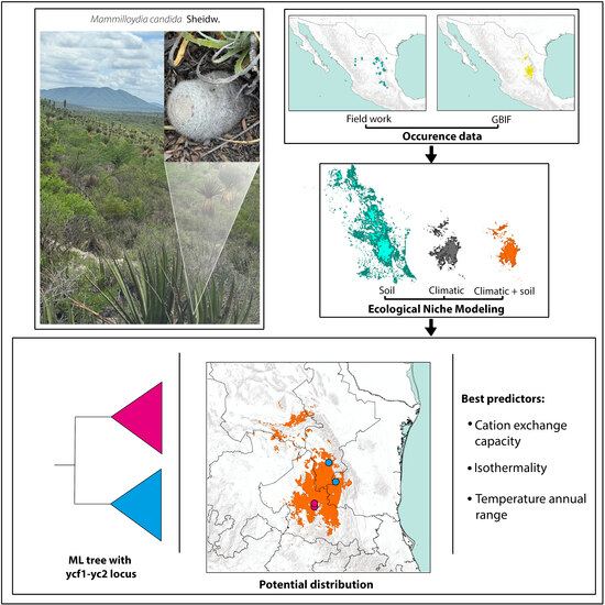
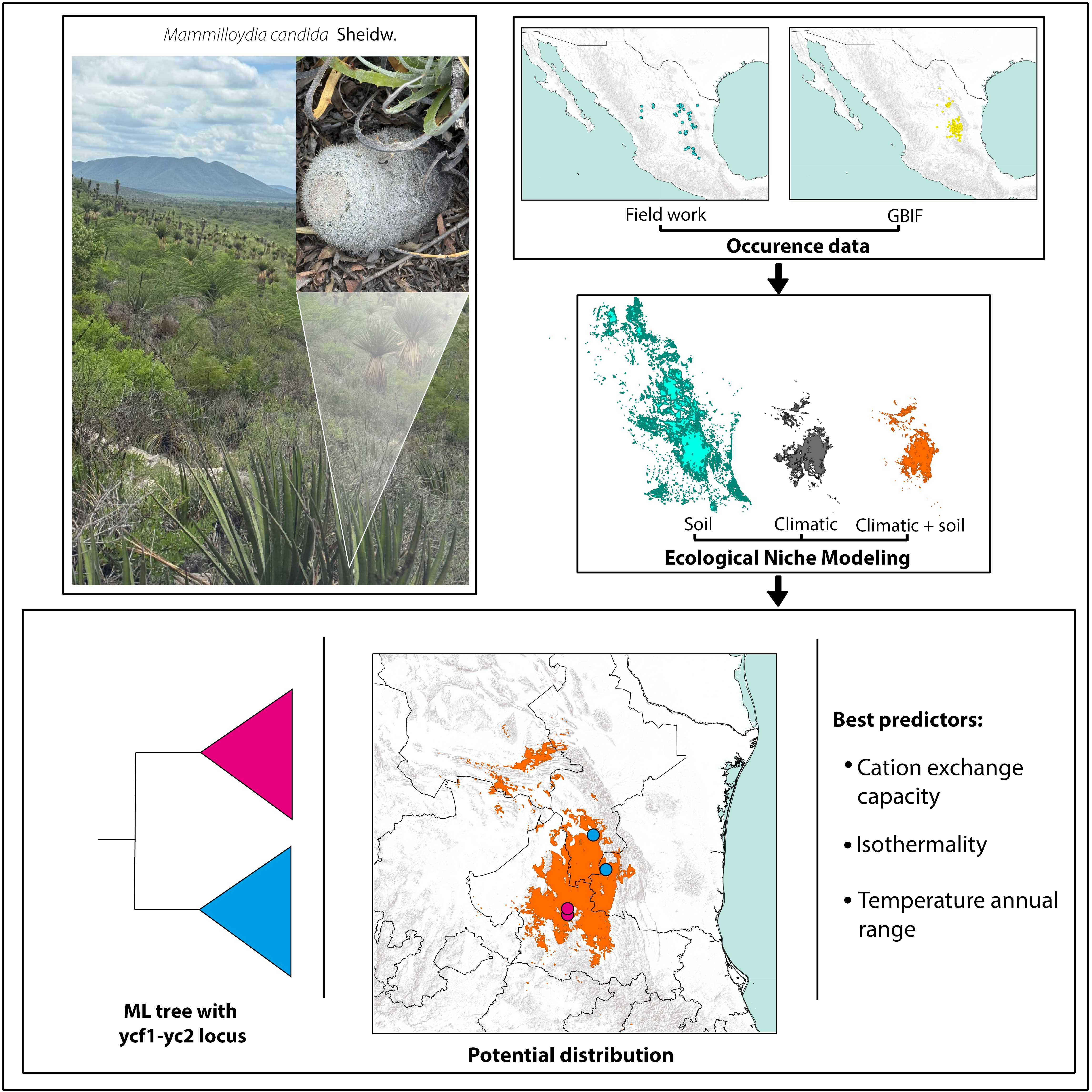
Graphical Abstract

1. Introduction

Assessment of the geographic range and levels of molecular variation of species produces pivotal insights that can be applied to conservation issues. Accumulated empirical evidence has demonstrated that niche-related processes and assembly rules (e.g., Ref. [1]) and specific life history traits significantly influence the geographic range of the species [2]. Microevolutionary processes (e.g., natural selection, gene flow, mutation, and genetic drift) are influenced by demographic factors [3]. Geographical range refers to a species’ spatial extension in a landscape and is related to the ecological niche [4]. Presently, most of the modeling procedures used to estimate the geographic range are based on occurrence points (occurrences), irrespective of whether these represent authentic biological populations or not; however, these produce accurate results about the real distribution of species [5].

Ecological niche modeling (ENM) provides an adequate framework for inferring the potential geographic distributions of species by combining known occurrence records with environmental variables. ENM can predict areas that are environmentally suitable for the species by projecting onto geographic space the environmental conditions that define a species’ ecological niche [6]. ENM can be used to infer potential geographic ranges (e.g., Ref. [7]), predict range shifts in climate change scenarios [8], and evaluate a species’ distribution’s environmental drivers [9]. Moreover, ENM has been widely applied in conservation biology to identify suitable areas for species translocation [10], prioritize conservation areas [11], and anticipate future range contractions [12].

Intraspecific molecular variation levels are used to determine conservation priorities, which are represented in an entire population or a small group of individuals. There are two types of conservation priorities: Evolutionarily Significant Units (ESUs) and Management Units (MUs). These types of units are operational tools for preserving genetic diversity when most taxa cannot be conserved across their entire geographic distribution. ESUs should be identified with a molecular marker that reflects the evolutionary history of the species (e.g., DNA sequences), and strong population divergence should be obtained in a phylogenetic tree. MUs are conservation units identified by significant divergence between populations based on genotype and allele frequencies and utilizing a variety of molecular markers, such as microsatellites, RAPDs, and some DNA sequences, with high variation rates [13]. This operative proposal, based on molecular variation levels to identify ESUs or MUs, has been widely applied in species in at-risk categories (e.g., Ref. [14]).

Niche modeling and molecular approaches have been integrated to assess distinct evolutionary topics (e.g., Refs. [15,16]), and the integration might have conservation applications (e.g., Ref. [17]), which was the purpose of this study by using an endemic and threatened species as a biological system.

The short-globose cactus, Mammillaria candida Scheidw., has been widely reported in the literature as Mammilloydia candida (Scheidw.) Buxb, but World Flora Online [18] establishes that the accepted name is Mammillaria candida. The International Union for Conservation of Nature’s Red List has classified Mammilloydia candida [19] as Least Concern since it is a widespread and abundant species and faces no major threats [20]. In contrast, the national Mexican Federal Normative (NOM-059-SEMARNAT-2010) listed this taxon as Mammillaria candida in the category of threatened [21]. Notably, neither of these two lists of species at risk referred to formal studies to justify these classifications.

The cactus M. candida is unambiguously reported to be endemic to Mexico. Hunt [22] documented this taxon in four Mexican states: Coahuila, Nuevo León, San Luis Potosí, and Tamaulipas. Guzmán et al. [23] additionally reported on these four states and Guanajuato, Querétaro, and Zacatecas. Other authors reported this taxon in Coahuila, Durango, Nuevo León, San Luis Potosí, Tamaulipas, and Zacatecas [24]. Barthlott et al. [25] also reported these Mexican states, except for Durango. Recently, González-Elizondo et al. [26] documented this taxon in Durango. The discordant geographic ranges of this cactus may be attributed to the limited fieldwork and the high morphologic variation it exhibits, which is reflected in the disputed nomenclature changes reported [18,23,27]. Whether such morphological variation hides probable cryptic species or lacks clear taxonomic circumscription with similar species remains unknown. The phylogenetic relationships of M. candida remain unclear.

Currently, molecular phylogenetic studies have identified different sister species for M. candida: Mammillaria herrerae Werderm. [28] and M. humboldtii C. Ehrenb. [29] based on plastidial loci; a cluster composed of five Mammillaria species [30] and M. albiflora (Werderm.) Backeb. [31]; De Vos et al. [32] identified Coryphantha as a sister lineage based on nuclear loci. Additional auxiliary data supporting taxonomic and phylogenetic issues is the assembled chloroplast genome because it is a specific trait [33]. In addition to its biological relevance, M. candida is a promising source of pharmaceutical compounds for the treatment of hypertension [34], and its extracts show a 92% reduction in tumor necrosis and antioxidant and anti-inflammatory activities [35].

Based on these antecedents, M. candida deserves attention for its conservation. In this study, we conducted intensive field surveys to support ecological modeling and document ecological information from natural populations. Ecological niches were modeled based on climatic and soil analyses to estimate the potential geographic distribution of M. candida. To identify genetic diversity and grouping, we estimated molecular variation through DNA sequences and microsatellite genotyping. These analytical perspectives were integrated to recommend conservation actions.

2. Materials and Methods

2.1. Fieldwork to Update Geographic Distribution and Tissue Sampling

Between 2023 and 2025, a total of 62 sites across nine Mexican states were visited (Table A1) to confirm the presence of M. candida in its reported natural habitats, collect tissue samples for molecular analysis, and document observations about local abundance from natural populations.

2.2. Review of Records to Derive a Dataset of Occurrence Points

Using the search terms “Mammilloydia candida” and “Mammillaria candida,” 690 instances were obtained from the Global Biodiversity Information Facility [36,37]. Using the rgbif package v. 3.8.1 [38] implemented in R v. 4.4.2 [39], these 690 entries were reviewed to remove duplicates, records with missing coordinates, and those with coordinate uncertainty greater than 1 km². Additionally, based on our field trips, we excluded all misleading reports (M. candida was absent). A final database of 254 curated records was used in the subsequent ecological analysis.

2.3. Ecological Modeling Based on Climatic and Soil Variables

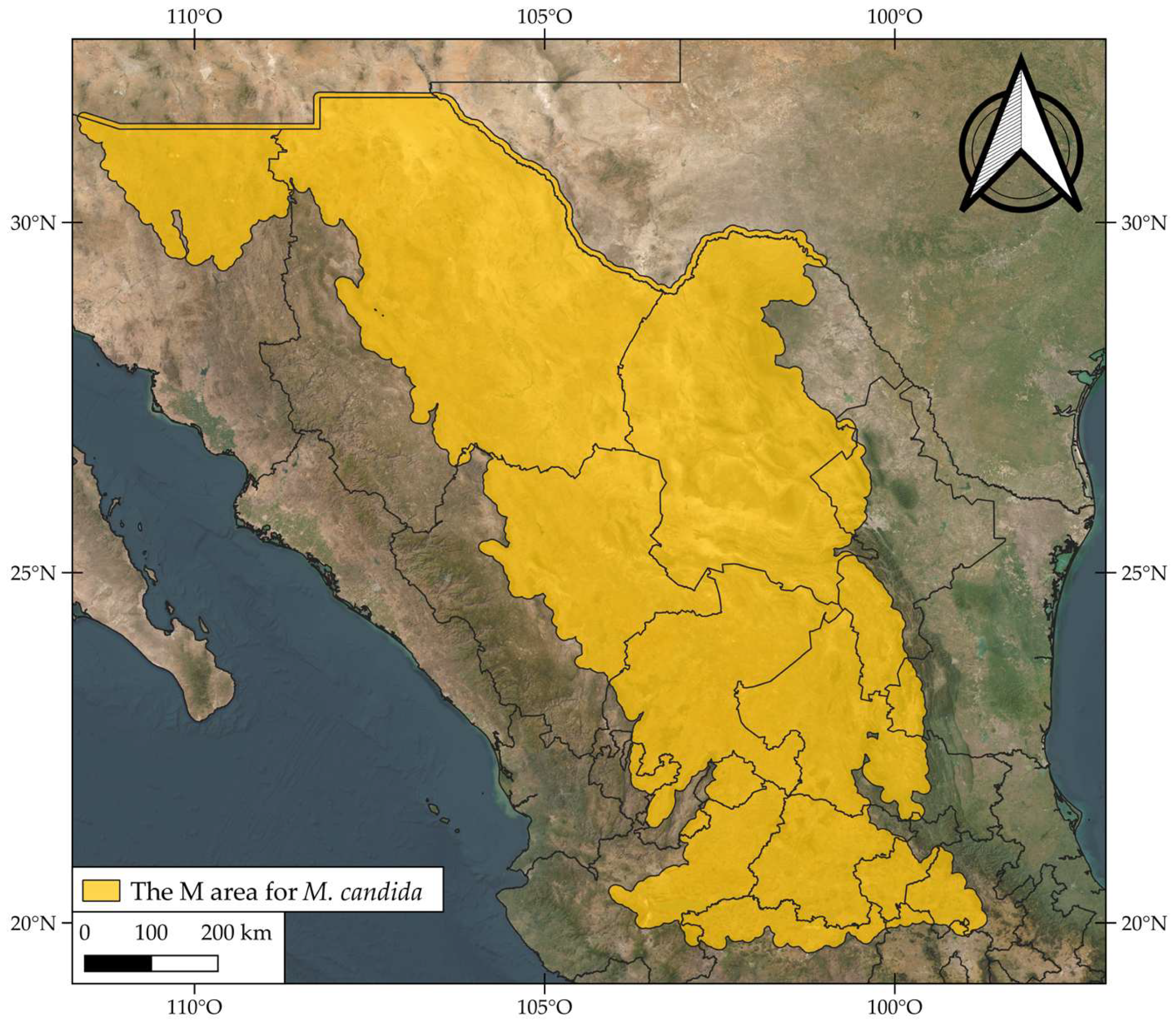
We estimated three ecological niche models based on (1) climatic variables, (2) soil variables, and (3) joint climatic and soil variables (climatic + soil, hereafter). All analyses were conducted in R using the packages indicated below. Nineteen bioclimatic variables were obtained from WorldClim v.2.1 [40], and eight soil variables for the 5–15 cm depth layer were downloaded from SoilGrids v.2.0 [41]. These 27 variables were obtained at a spatial resolution of 1 km². According to values less than 10 of the variance inflation factor (VIF) estimated with sdm package v.2.7-1 [42], seven climate and eight edaphic variables were selected for subsequent analysis (Table A2 and Table A3). The accessible area (M) was identified using 254 curated occurrences, following the BAM framework by Soberón and Peterson [43]. This area corresponded to the Mexican portion of the Chihuahuan Desert sensu Escalante et al. [44] with a 10 km buffer (Figure A1). This area M was used to calibrate each of the three ecological niche models (ENMs). The ENMs were generated using MaxEnt v.3.4.3 [45], which was implemented using the kuenm v.1.1.1 package [46]. The modeling workflow consisted of three steps: (1) A total of 651 candidate models were calibrated using combinations of parameters of feature classes and regularization multipliers (Table A4). (2) The selection and validation of the most suitable model were based on statistical significance, partial receiver operating characteristic (pROC) tests, omission rates (ORs) < 5%, and the lowest Akaike Information Criterion corrected for small sample sizes (AICc). (3) Continuous suitability outputs were transformed into binary presence–absence predictions using the 10th percentile training presence threshold (see Appendix B for additional details). The predictor power of the best model was tested with the metrics of sensitivity, specificity, and the True Skill Statistic (TSS) using Terra package v. 1.8-60 [47].

2.4. Estimation of the Area Included in the Protected Areas System

The model with the highest predictor power was used to estimate the overlapping surface included in the Natural Protected Areas (NPAs) of Mexico [48]. This area overlapped among NPAs, and the best model was estimated using the Terra package.

2.5. Molecular Analysis

2.5.1. DNA Isolation and Sequencing

Fresh tissue was collected from 3–20 individuals during the fieldwork according to the density of M. candida per site. Each sample was individually preserved in plastic bags with silica gel desiccant. The total genomic DNA (gDNA) was isolated from 20–30 mg of dry tissue, following the instructions provided in the manual of the DNeasy Plant Mini Kit (Qiagen, Germantown, MD, USA). Total gDNA was verified in 1% agarose gels and visualized in UV light. The locus ycf1–ycf2 was sequenced for 20 samples using the primers F: 5′ GGC ATC TTG AGA GTG ATT CGT and R: 5′ CTG GCT AAC ATA GAA CTT GGG A, which were designed following the bioinformatic processing described in Appendix E from raw data available at NCBI (SRR23441692, referenced in [30]). For microsatellite markers, 95 samples were genotyped following the conditions described in Appendix F and Table A5.

Both PCR amplifications of sequencing and microsatellite reactions were processed in the 2720 Thermal Cycler (Applied Biosystems, Foster City, CA, USA). PCR amplicons of 500 bp were sent to a sequencing provider, who prepared the sequencing reactions with the BigDye Terminator v3.1 Cycle Sequencing Kit and sequenced them in the DNA Analyzer 3730xl. With this equipment, we also performed the electrophoresis of microsatellite fragments (Applied Biosystems, USA).

2.5.2. Statistical Analysis

Phylogenetic Analysis

Forward and reverse sequences obtained for each of the 20 samples were joined into a single sequence in SeqTrace v.0.9 [49]. These sequences were aligned in MAFFT v.7.453 [50] to identify the different haplotypes. The genetic relationships among the haplotypes were estimated using a TCS network [51] using popART v.1.7 [52]. The outgroup was Mammillaria albiflora, whose sequence was previously reported (MN517610.1 [33]).

Estimation of Population Diversity and Structure

Microsatellite data were used to describe genetic diversity and structure. Most of the statistical estimators were obtained in Arlequin v. 3.5 [53] and GenAIEx v. 6.51 [54], as well as in adegenet package v. 2.1.11 [55] in R v. 4.4.2 [39]. We organized the data to execute statistical analyses per locus across the eight sampled sites to estimate genetic diversity at the species level, whereas the results of the five loci were used to describe the population level. The expected and observed heterozygosity were estimated for the species and each of the eight populations, and the inbreeding coefficients were estimated following Nei’s [56] equations implemented in Arlequin. Deviations from the Hardy–Weinberg Equilibrium were calculated following the procedure developed by Guo and Thompson [57], which is based on Fisher’s exact test with 1 million Markov chains implemented in Arlequin. The total number of alleles, mean number of alleles per locus, and effective number of alleles were estimated using GenAIEx. We identified private alleles for each locus and population using the adegenet package v. 2.1.11 [55]. The probability of a bottleneck was estimated using the Garza–Williamson index (G-W) included in Arlequin. The population structure in Arlequin was estimated with the differentiation index adjusted for microsatellites (R_ST). In GenAIEx, we estimated Principal Coordinate Analysis (PCoA) based on the genotypes of 95 samples. Nei’s genetic distances between populations were used to develop a neighbor-joining tree for genetically diverse populations using ape-package v. 5.8-1 [58]. The isolation-by-distance gene flow model was tested with a Mantel test implemented in vegan package v. 2.7-3 [59] in R. To estimate the sources of variation, an AMOVA test was performed in Arlequin. Then, the eight sites were grouped as follows: Group 1 comprised sites from San Luis Potosí, Group 2 comprised samples from Tamaulipas, and Group 3 comprised samples from Coahuila and Nuevo León.

3. Results

3.1. Fieldwork Surveys

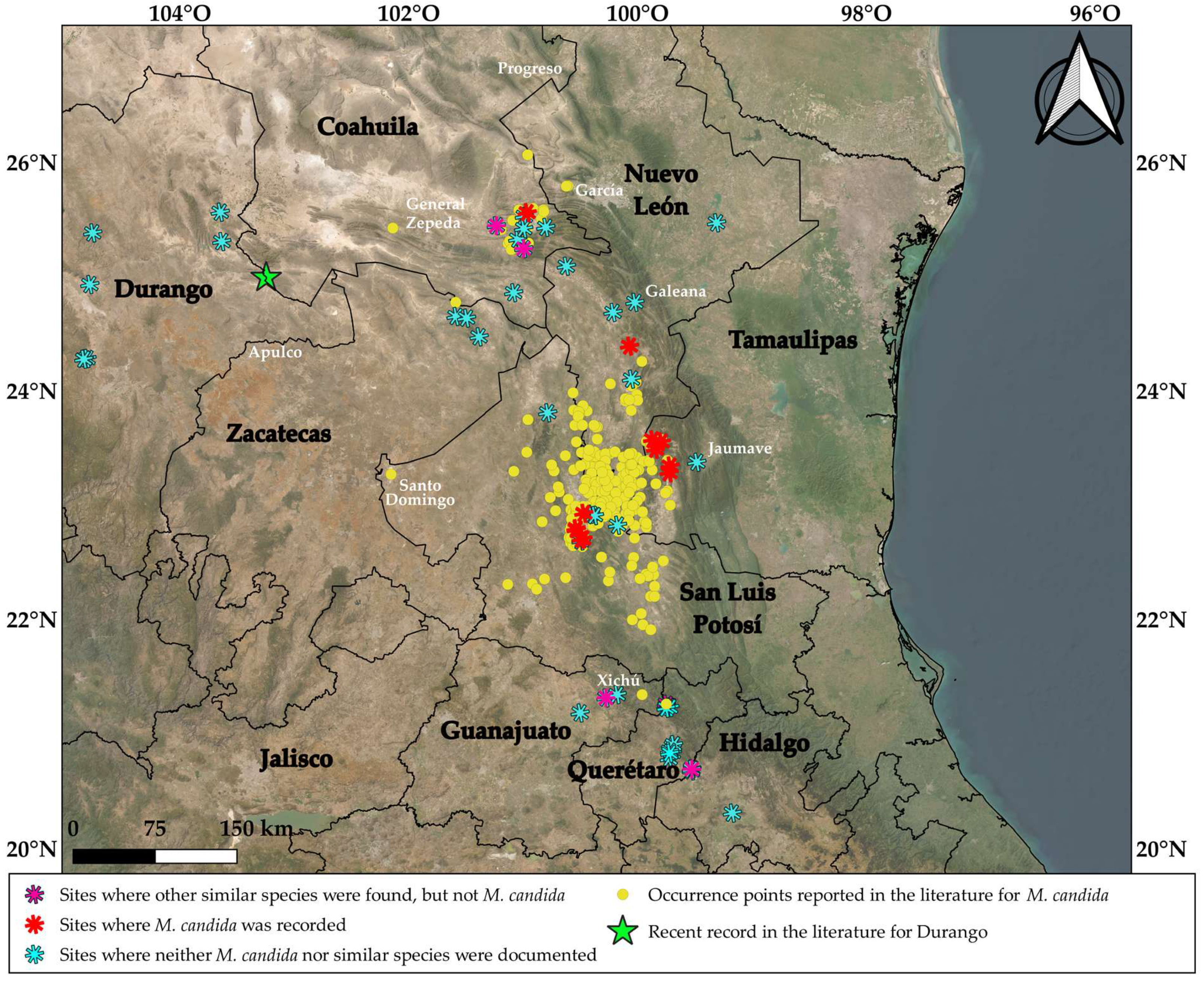
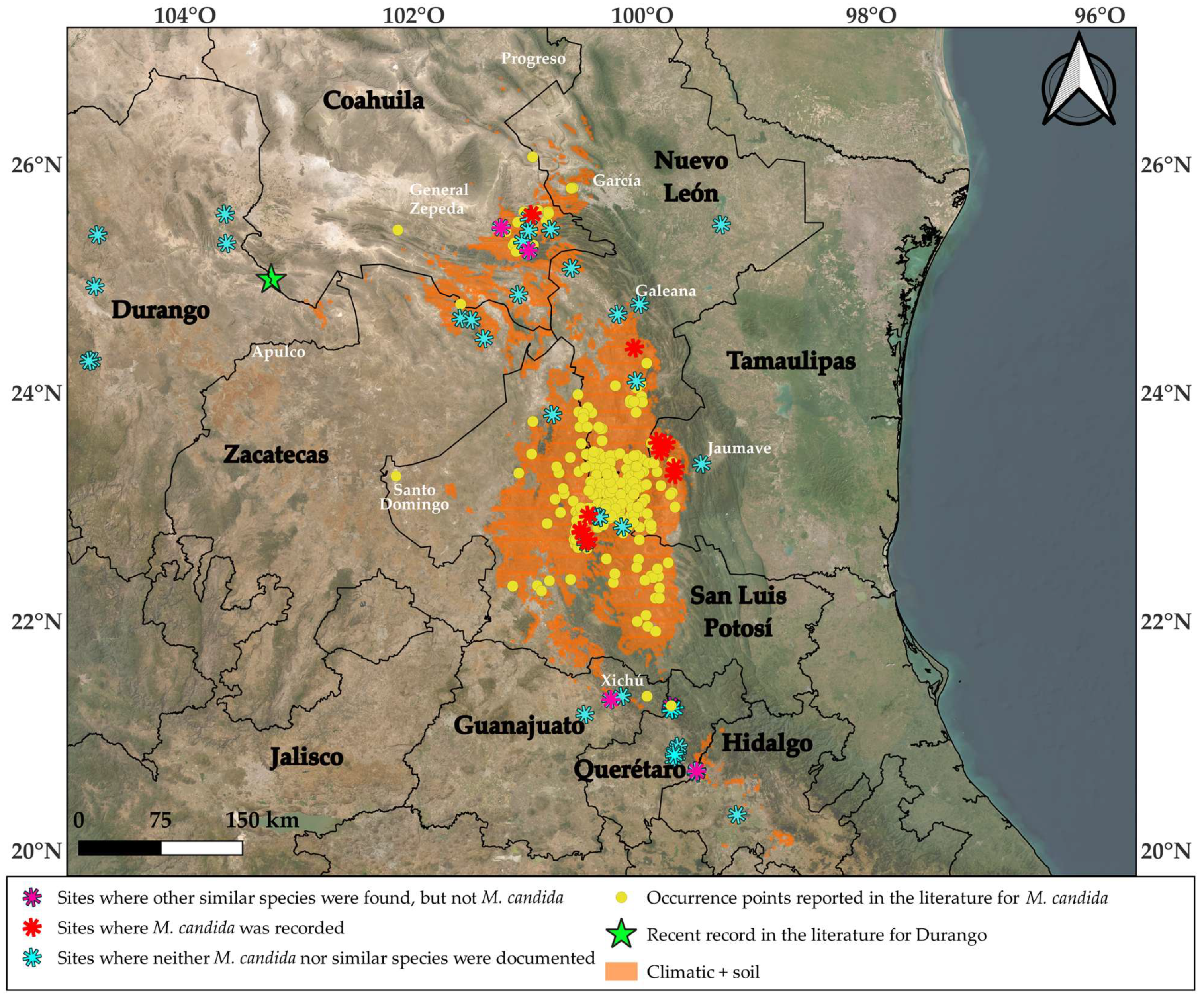
Fieldwork confirmed that M. candida is native to the arid interior of the Chihuahuan Desert and is limited to four Mexican states, namely, Coahuila, Nuevo León, San Luis Potosí, and Tamaulipas (Figure 1). Other taxa, but not M. candida, were documented with specific coordinates in many sites where this taxon was reported (pink asterisks in Figure 1).

In Guanajuato, we documented Mammillaria geminispina Haw. in those sites reported in the municipality of Atarjea, and in the surrounding sites reported close to the small village of Xichú, M. muehlenpfordtii C.F. Först. was documented. M. grusonii Runge was recorded at several sites in Coahuila and Durango. In addition, we documented M. lasiacantha Engelm in some sites in Durango and Nuevo León. In various localities of Coahuila, Nuevo León, San Luis Potosí, and Tamaulipas, M. formosa Galeotti ex Scheidw. was found, but not M. candida. The presence of this taxon was not confirmed in the state of Querétaro because the three reported sites were transformed into residential areas and private ranches.

Of the curated occurrences (254), most (53%) were in San Luis Potosí (Table 1, Figure 1), and during fieldwork, we confirmed that this state harbored most of the populations of M. candida.

Our results indicate that San Luis Potosí harbors the southernmost and easternmost populations of M. candida, while Tamaulipas marks the northeastern distribution along the extensive Jaumave Valley, and Coahuila represents the northernmost limit of the species’ geographic range (Figure 1). In the arid lands of Coahuila, we did not document abundant populations, only a few individuals (three–nine). In contrast, in Nuevo León, San Luis Potosí and Tamaulipas, some sites harbored abundant populations of 20–50 plants, as well as very abundant populations of over 100, but most individuals were aggregated into small areas of roughly 100 × 100 m on the foothills of the mountains. We documented that this taxon occupied an elevation range that varied from 1140 m (Jaumave) to 2160 m (Miquihuana) (Table A1).

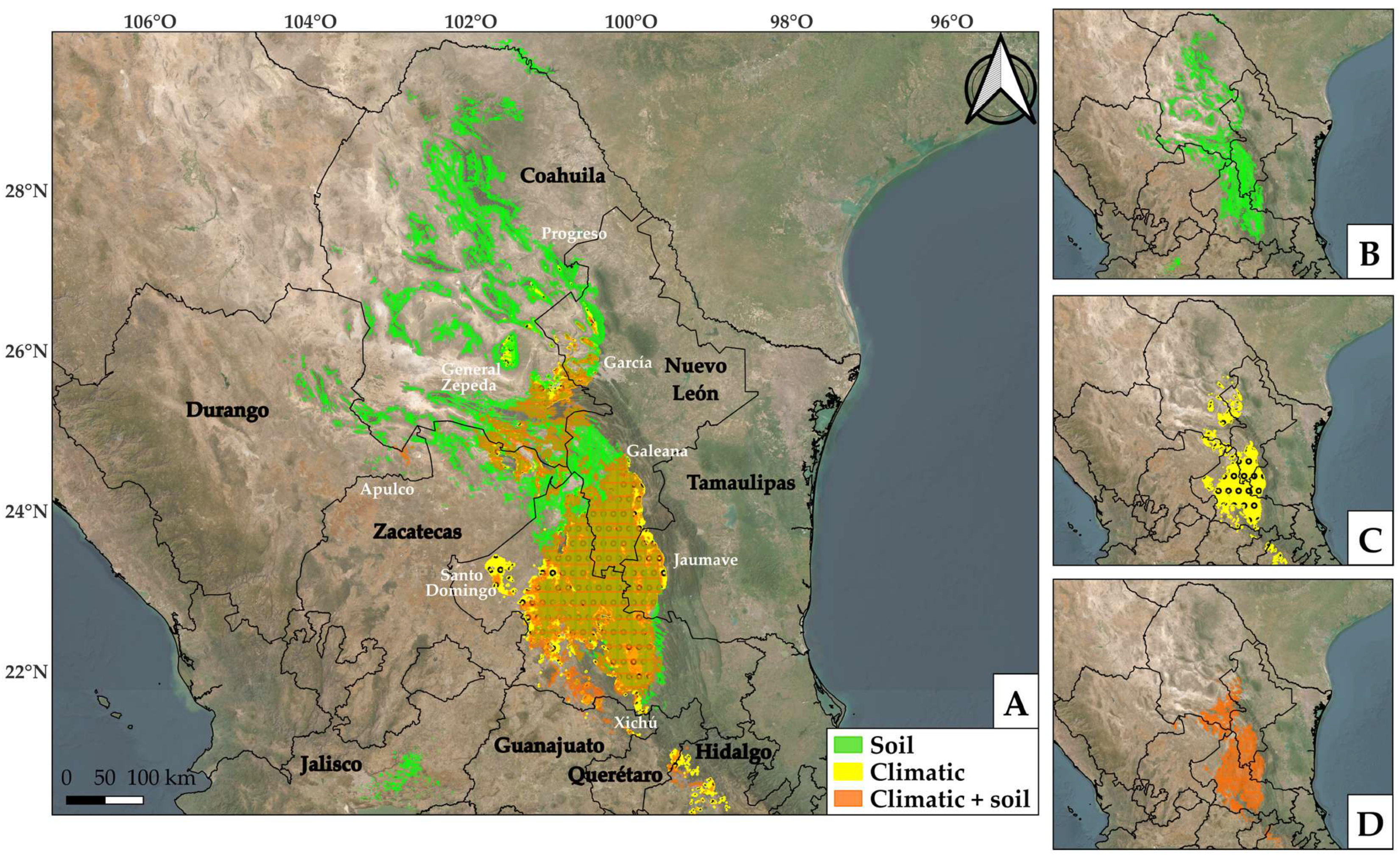
The typical vegetation type occupied by this taxon was rosetophyllus desert scrub. In the dense vegetation of thorny scrub, most M. candida individuals were documented under the shadow of short shrubs, Yucca, Opuntia, or immersed in patches composed of Agave, Hechtia, or Nolina. M. candida was rarely documented in open sites without vegetation, and on steep cliffs, it did not grow on naked rocks but in rock fissures, where a small microhabitat with soil and humidity was available. Our fieldwork results were very concordant with the projected areas of the two ecological models (Figure 2), particularly those estimated using the climatic + soil model.

3.2. Potential Geographic Distribution

According to the partial ROC and its associated omission rate value, the three ecological models were statistically robust (Table 2). In addition, each of the three models mostly estimated a continuous polygon enclosing dense occurrence points (Figure 1). However, during the fieldwork, we did not document a continuous distribution pattern but rather the geographically isolated hills occupied by M. candida.

We discarded the model based solely on edaphic variables, as it largely overestimated (77,082.23 km²) the potential geographic distribution (soil model in Figure 2). This model projected the edaphic environment in distant and non-desertified areas (Jalisco) and the largest portion of the state of Chihuahua reaching the Mexican–USA border. However, there were no records indicating that M. candida is distributed in either Jalisco or Chihuahua.

On the other hand, the climatic and climatic + soil models were accurately adjusted for occurrences as well as sites verified in the fieldwork (Figure 1 and Figure 2). However, the climatic model projected the distribution to the north of Ramos Arizpe, where only two occurrences were reported. In contrast, climatic + soil projected other small areas northeast of Nuevo León (Figure 2). These two models projected a small area to the eastern portion of San Luis Potosí, but it was far from a single occurrence (Santo Domingo municipality; Figure 2). However, in this portion, the climatic model projected a larger area than the climatic + soil model. In Guanajuato, Hidalgo, and Querétaro, the two models forecasted a few, small and scattered areas, whereas the climatic model predicted a greater number and larger size of these areas (Figure 2). These two models projected an area on the surrounding territories where the boundaries of Coahuila, Nuevo León, San Luis Potosí, and Zacatecas converged (Figure 2), but no records supported this area. In addition, the climatic + soil model estimated a mostly identical area (37,519 km²) to that of the climatic model (35,964 km²), but the former had a small additional area, which is mostly located in Durango (Figure 2). In addition, the climatic + soil model projected two areas without previously reported occurrences, and one of these areas was in Nuevo León, which was corroborated during fieldwork. These results indicate that the interaction of climatic and edaphic variables is correlated with the geographic distribution of M. candida; this model had the best fit according to occurrence points and fieldwork (Figure 3).

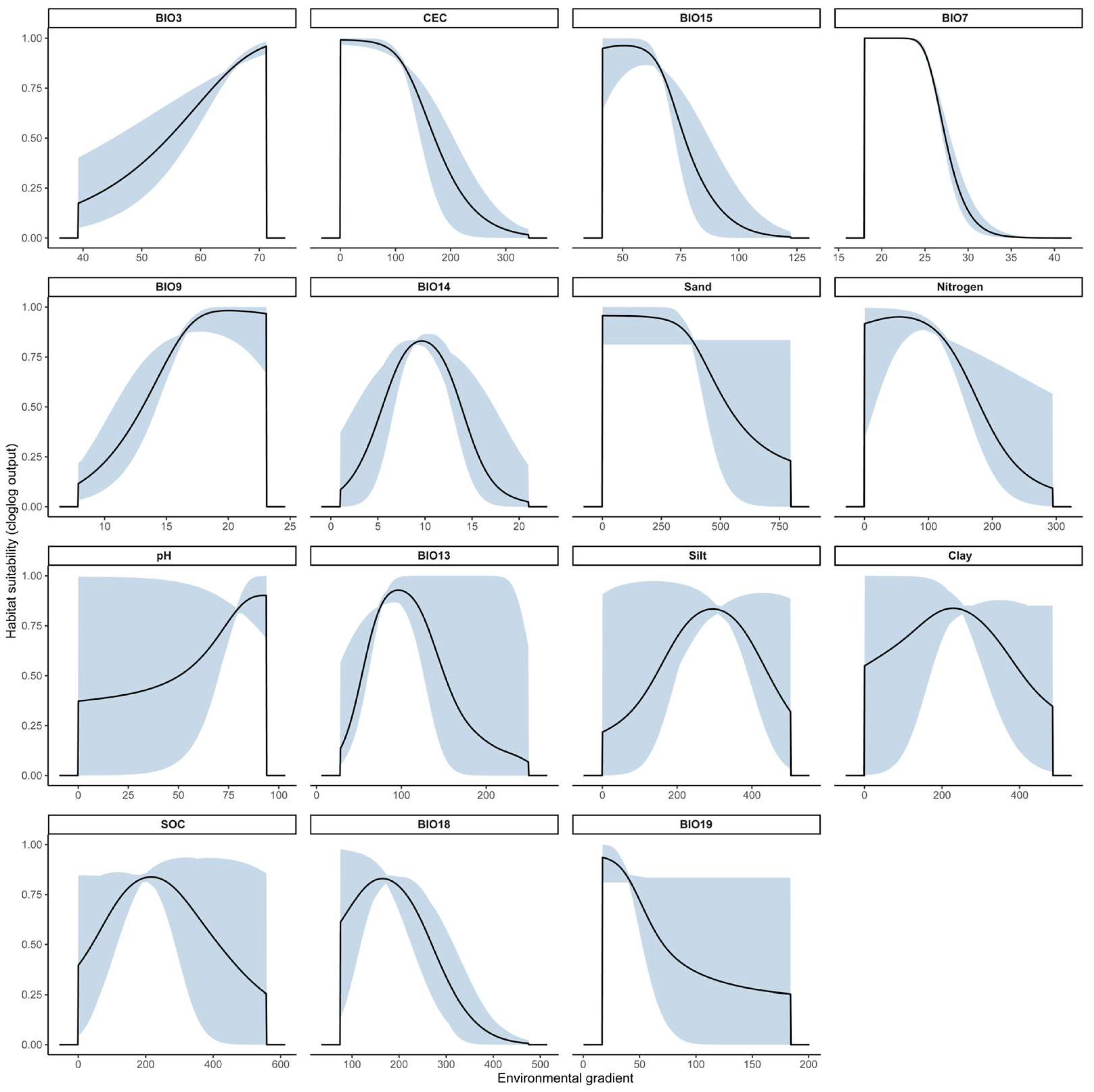
The climatic + soil model had the best power predictor, as indicated by pROC (1.93), AICc (2639.12), and TSS (0.82) values (Table 2). The response curves of environmental variables for the best ecological niche model, including habitat suitability (Figure A3), showed that the five influential variables indicated a suitable isothermality (BIO3) of 60–70, a CEC (0–150 mmol(c)/kg) along with precipitation seasonality (BIO15) of 25–75 mm, a temperature annual range (BIO7) of 18–25 °C, and a mean temperature of the driest quarter (BIO9) of 16–24 °C. This model predicted an M. candida range in the arid Chihuahuan Desert areas, as well as along the Sierra Madre Oriental’s foothills of the oriental continental plateau.

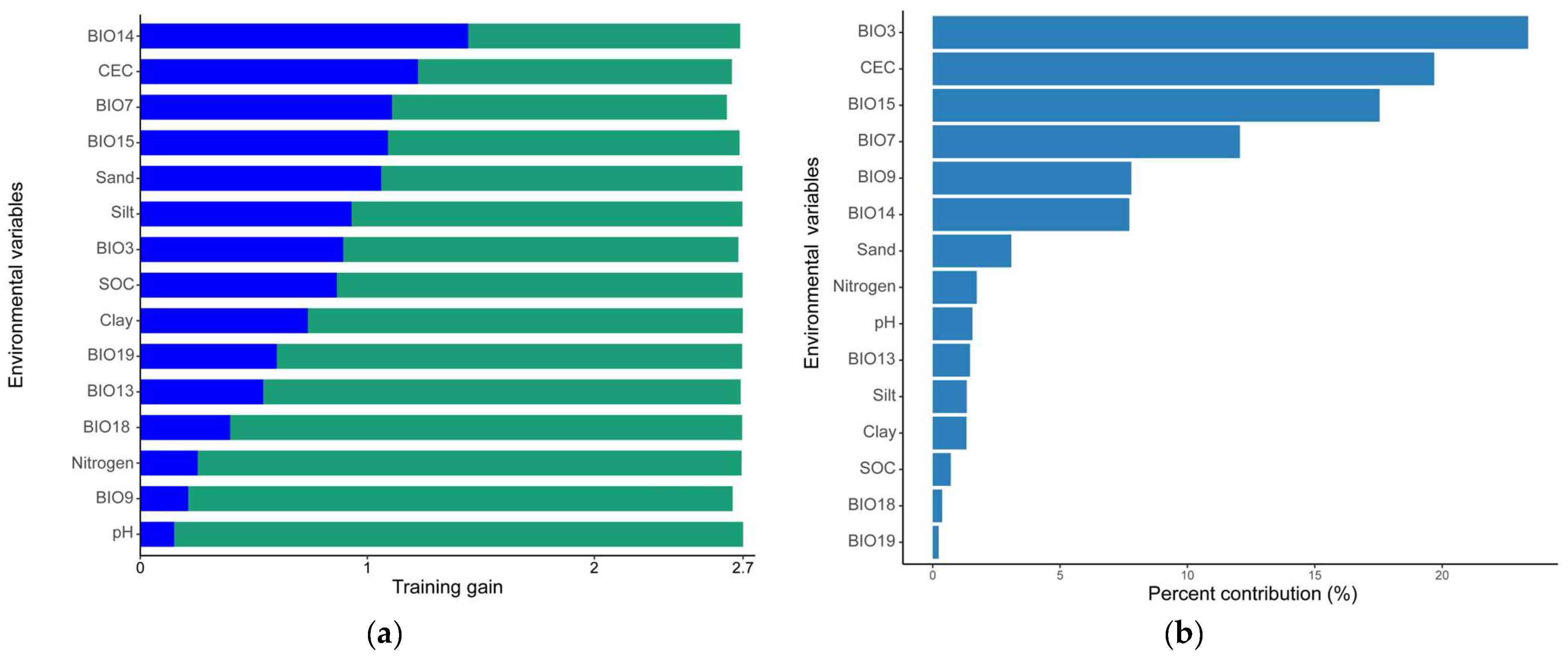
The Jackknife results (Figure 4a) showed that the most important predictor variables were BIO14 (precipitation of the driest month), CEC (cation exchange capacity), BIO7 (temperature annual range), BIO15 (precipitation seasonality), and sand (proportion of sand particles). However, the results revealed that the variables that made the highest contribution to the model were BIO3 (isothermality), which contributed 23.49%; CEC (19.7%); and BIO 15 (17.5%), BIO7 (12.1%), and BIO9 (mean temperature of the driest quarter, 7.8%) (Figure 4b). Accordingly, these variables of temperature and precipitation, as well as the soil properties of CEC and sands, were correlated with the geographic distribution of M. candida.

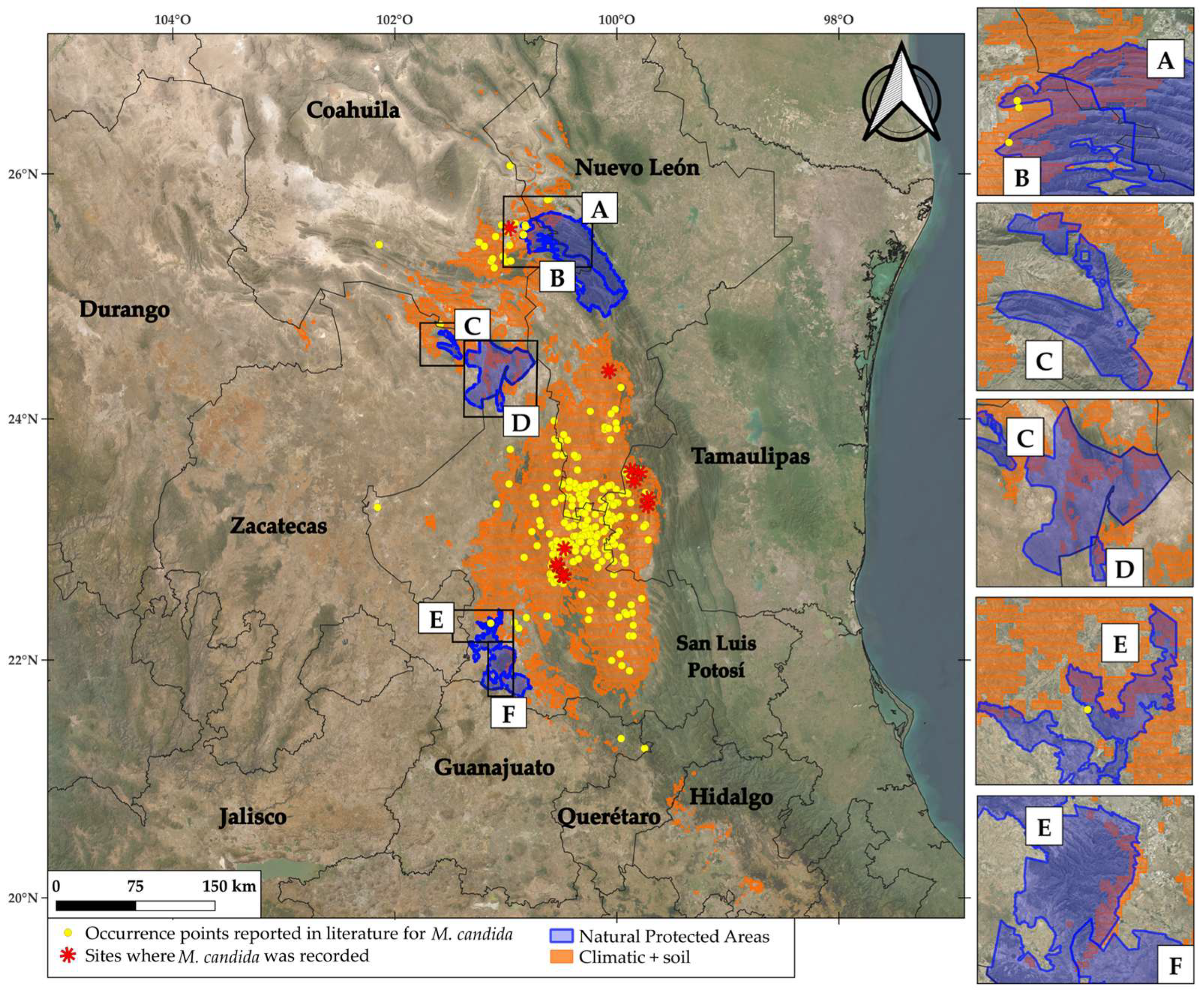
In contrast, a comparison between the model estimated by climatic and soil variables and the decreed Mexican Natural Protected Areas (NPAs) showed that only 1.45% of the surface of the potential distribution was included in some of the six NPAs located in four Mexican states. However, this surface corresponded to the modeled area, and no occurrences or field-documented sites were located on any of the six NPAs (Figure 5).

3.3. Phylogenetic Relationships

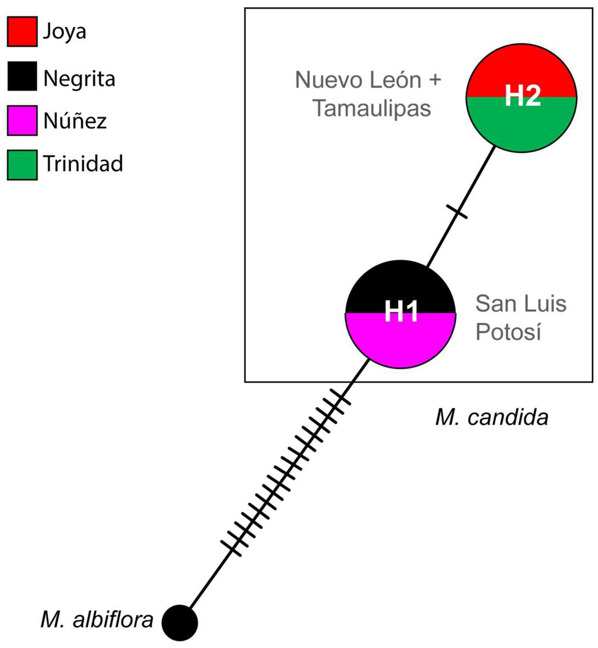
The ycf1–ycf2 locus analysis divided the 20 samples into two distinct groups (Figure 6): one containing all individuals from San Luis Potosí, and the other encompassing those from Nuevo León and Tamaulipas. Furthermore, each of these two groups (San Luis Potosí and Nuevo León + Tamaulipas) was characterized by a single haplotype.

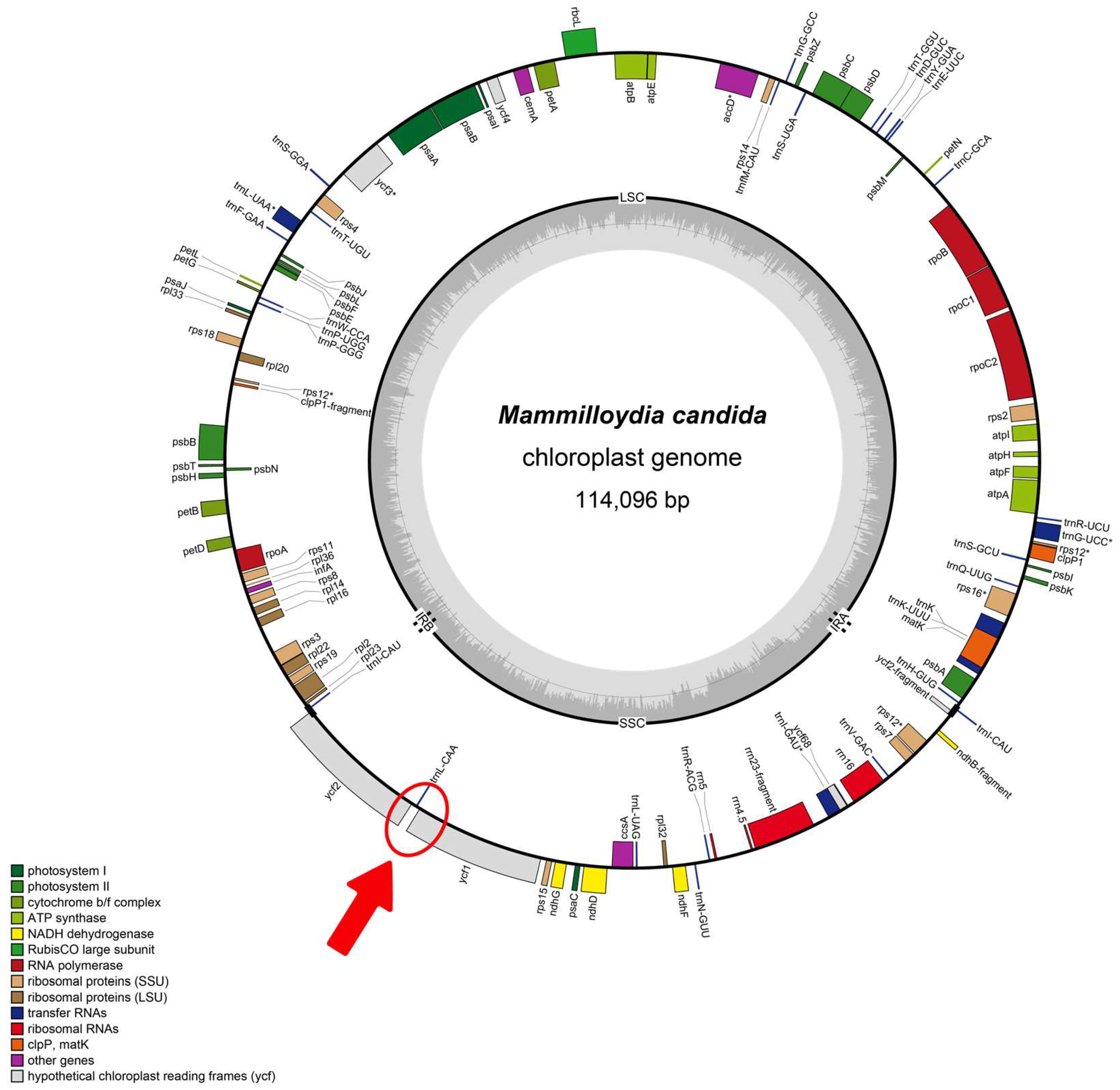
A secondary result obtained using the assembled complete plastid genome was that it has the shortest inverted repeats reported for cacti (Figure A2). These inverted repeats (IR_A and IRA_B) were 583 bp in length, were identical in DNA sequence, and comprised the trnI^CAU-ycf2-fragment. In addition, this sample had haplotype H1 like the samples from San Luis Potosí.

3.4. Population Diversity and Structure

For M. candida, the total expected heterozygosity was higher (H_T = 0.87 ± 0.11 SE) than the observed heterozygosity (H_I = 0.81 ± 0.12). In this species, the inbreeding coefficient was moderate and significant (F_IT = 0.14, p = 0.01). The total number of alleles identified in the species by the five loci was 138, and the mean number of alleles per locus was 27.6 ± 3.7. Locus MamVTC9 identified the lowest number of alleles (Table 3). The global test of differentiation did not estimate differences among the sampled populations (R_ST = 0.11). The results did not support a bottleneck that occurred in this taxon, since the G-W index had a low value and was not significant (0.30, p = 0.08).

The number of individuals analyzed at the population level (Table 4) ranged from 2 (Arizpe) to 20 (Calabacillas), which was influenced by both the number of individuals found in the location and problems with PCR that affected data retrieval. Discarding Arizpe and Jaumave for comparative diversity purposes, the results suggest that the populations have relatively high levels of genotype and allele diversity, with Trinidad (Nuevo León) and Calabacillas (Tamaulipas) being the populations with the highest levels of observed heterozygosity. In addition, Calabacillas stood out among all the descriptors of allelic diversity (Table 4). Interestingly, all sites harbor private alleles, but Calabacillas (20) and Trinidad (13) have the highest numbers. Moreover, even the two geographically closest sites (~12 km in distance), Negrita and Núñez, have private alleles. All populations showed a lower effective number of alleles than the total or average number of alleles per locus, suggesting that these low-number alleles effectively contribute to the levels of heterozygosity. The results did not support the notion that a bottleneck occurred in some of the eight sites since the estimated values of the G-W index (Table 4) were not distinct from zero (p < 0.05).

In contrast, the paired comparisons of differentiation index (R_ST) values indicated weak-to-moderate genetic differentiation between populations, although most of these values were not statistically significant (Table 5). Most significant R_ST were identified in Núñez, and it had the lowest gene flow levels (above the diagonal in Table 5) except for Negrita (Nm = 15.85), which is the closest geographical site.

In addition, levels of gene flow between populations were high (Table 5, above the diagonal). The studied populations did not adjust to the isolation-by-distance gene flow model (Mantel R = 0.246, p = 0.147). Therefore, the significant differences in R_ST values shown in Table 5 were not directly related to the geographic distances between the sites. An interesting outcome is that Núñez was statistically distinct from the other sites (R_ST values below the diagonal in Table 5), and this site had the lowest gene flow values, except for Negrita, which was the closest to it (Table 5). The AMOVA test estimated 88.8% variation within populations, followed by variation among groups (7.5%) and variation among populations within groups (3.7%). Accordingly, the source of genetic variation in M. candida is contained at the level of the population.

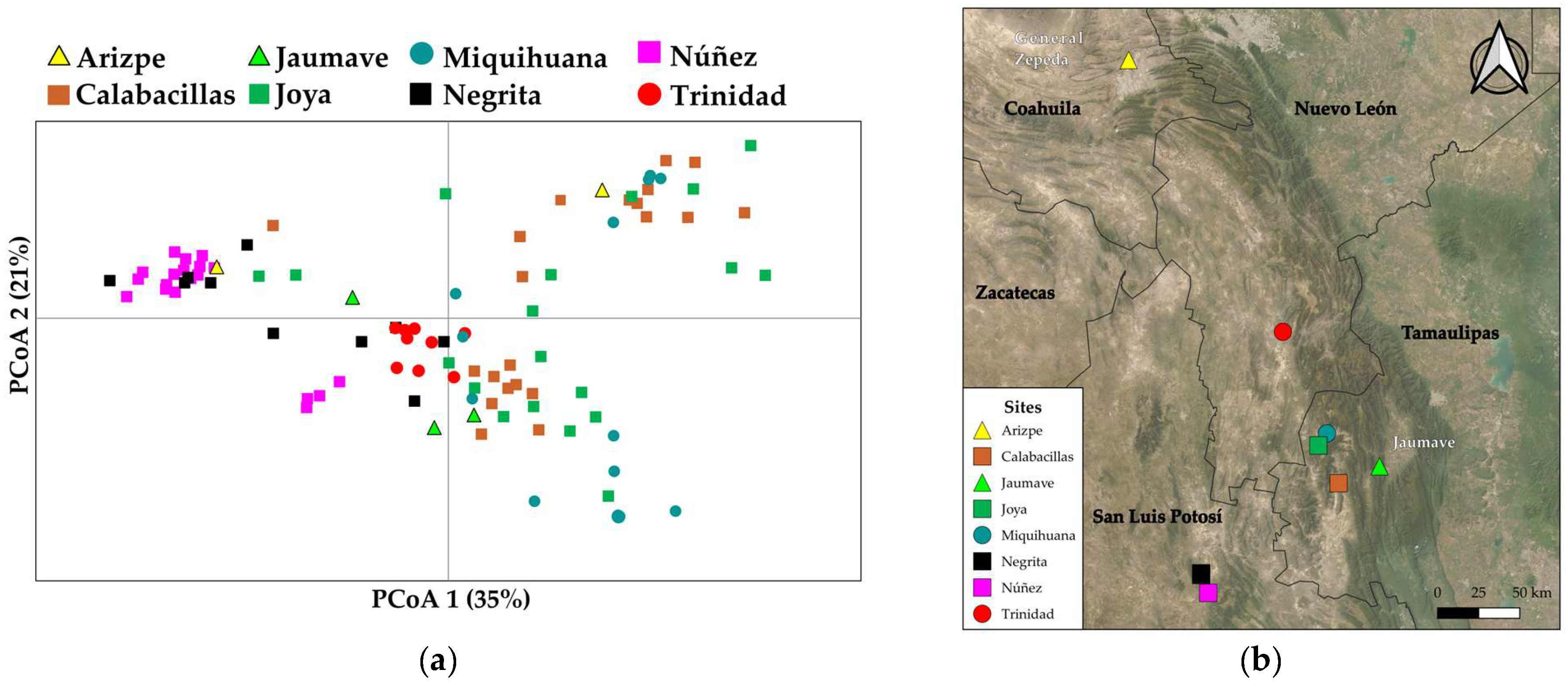
On the other hand, the PCoA identified a clear structure based on the similarities of the genotypes. Two axes added 56% of the variation provided by the genotypes identified by microsatellite loci (Figure 7a). These axes separated most of the genotypes from Tamaulipas (Calabacillas, Joya, and Miquihuana) and San Luis Potosí (Núñez and Negrita). In addition, the PCoA revealed that genotypes from Nuevo León (red points) tended to be concentrated close to the origin (0, 0), in the IV quadrant. These genotypes were intermediate between a group from Tamaulipas and a group from San Luis Potosí (Figure 7b). Genotype migration was also detected in this analysis, as several genotypes were closer to genotypes that are not of the same geographic origin. This genotype migration was identified for all sites, except Nuevo León (Trinidad). Although the number of samples from Jaumave (Tamaulipas) and Arizpe (Coahuila) was very low, the PCoA related these genotypes to Tamaulipas and San Luis Potosí (Figure 7b). Part of the genotypes from Negrita were close to Núñez, but others were to those from Nuevo León. This analysis suggests three genotypic groups: (1) Calabacillas–Joya–Miquihuana, (2) Trinidad, and (3) Núñez–Negrita.

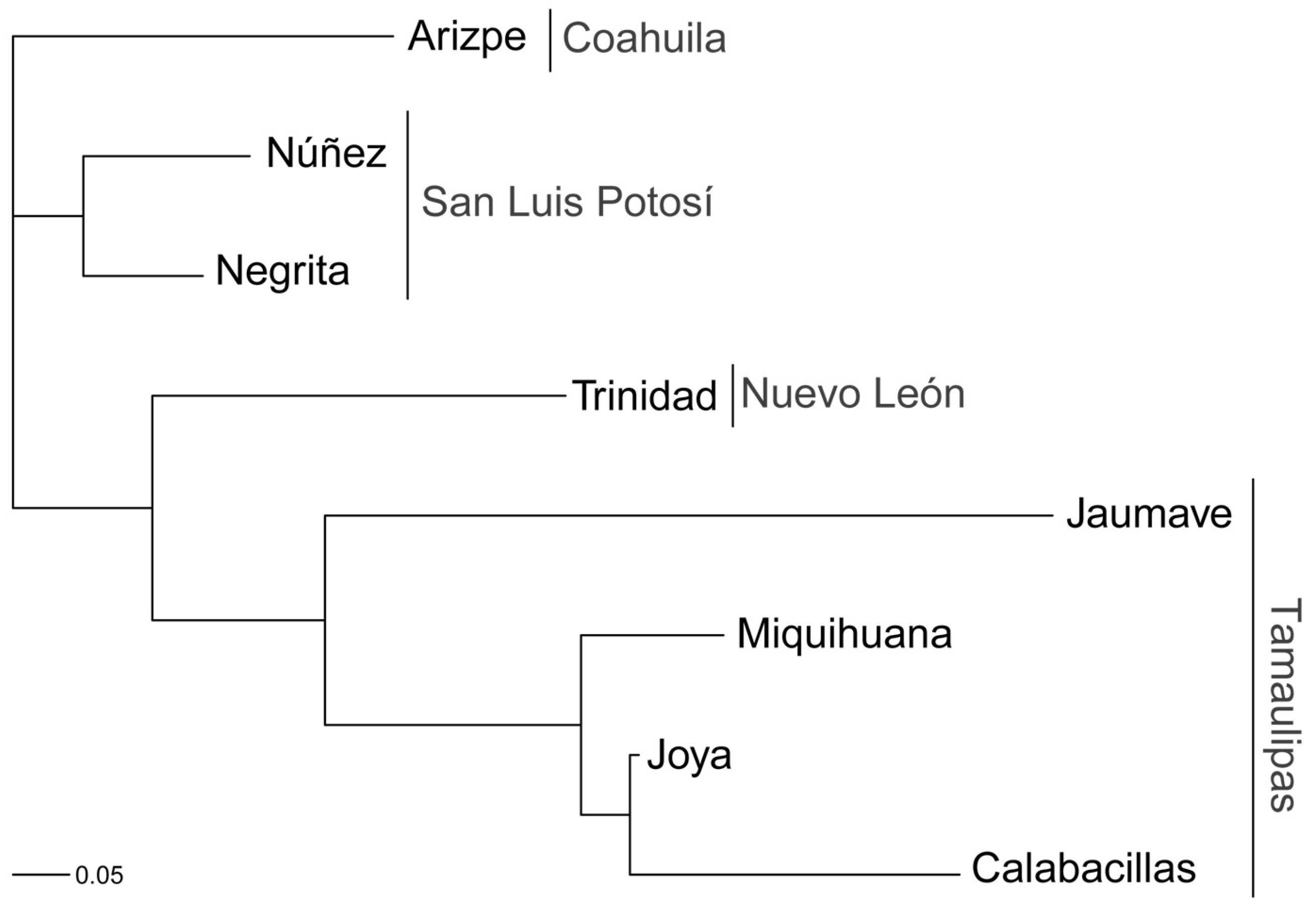
Nei’s genetic distance showed that the four sites in Tamaulipas were clustered together, whereas Trinidad in Nuevo León was positioned between Tamaulipas and San Luis Potosí, as indicated by Negrita–Núñez (Figure 8). Arizpe (Coahuila) branched out with San Luis Potosí and Nuevo León. Populations were grouped mostly according to their geographic origin, then the two sites from San Luis Potosí were branched together, and Nuevo León was genetically closer to Tamaulipas. Since only two samples were genotyped for Arizpe, its position was unclear.

4. Discussion

The results of this study showed that M. candida is endemic to the interior of the Chihuahuan Desert and restricted to four Mexican states: Coahuila, Nuevo León, San Luis Potosí, and Tamaulipas, which is concordant with Hunt [22]. However, our results contrast the geographic distribution reported by other previous studies [24,25], which extended the distribution range of this taxon to Durango and Zacatecas. In these two states, fine-scale field verification is necessary, and we recommend taking as a guide the projected distribution of the climatic + soil model, since it was highly precise. Regarding Guanajuato, we visited sites that were reported with herbarium specimens and attached coordinates; however, we found sites where other similar species of Mammillaria but not M. candida were recorded. Since these specimens were collected before 2000, GPS errors are probable. On the other hand, those sites reported for Querétaro were transformed into residential and private properties and thus no longer constitute natural habitats. We detected that many false reports referred to other Mammillaria species or even cacti of other genera; they were caused not only by the high morphological variation across its entire geographic distribution, which has been reflected in its nomenclatural history [26], but also by the lack of a clear taxonomic circumscription. Accordingly, we suggest that future studies employ an integrative taxonomic approach that includes morphological analysis across the entire geographic distribution, fine-scale descriptions of habitats, demographic monitoring, pollination biology and seed dispersion, well-resolved phylogenetic trees, and complete assembled genomes. In this study, we reported for a single specimen of unknown geographic origin the assembled and annotated plastid genome whose inverted repeats have a distinct structure from those previously published for Mammillaria species but are very similar to those reported for M. albiflora [33], identified as a sister species in a published phylogeny [30].

According to our results, niche modeling was a powerful tool to estimate the geographic range of M. candida, but we recommend, as indispensable steps, a detailed scrutiny of occurrences reported in GBIF [36,37], a detailed review of herbaria specimens, and if possible, field inspections. The model obtained using only soil variables overestimated the ecological niche of M. candida. We consider that this occurred because the modeling identified similar edaphic conditions in the M area; however, there are no other conditions that circumscribe the ecological niche of this cactus, as was evident in the area projected on Jalisco and Chihuahua. However, the results obtained here show that it is not the individual sets of variables but the interaction of climatic and soil variables that allows us to understand the distribution of this cactus.

The climatic + soil model projected areas in Coahuila and Nuevo León, and one of these was confirmed in this study. Therefore, it is recommended that those other projected areas, which were not supported by occurrences, be inspected in future studies. Particularly, those small, scattered areas projected on Guanajuato–Querétaro, because in the past (before 2000), specimens classified as M. candida were collected. Moreover, the populations described as the subspecies M. candida caespitosa north of Saltillo [24], as well as other varieties and subspecies reported in the literature [23,27] and atypical records [25] located in areas where the suitable environment was not projected, deserve special taxonomic studies.

The climatic + soil model had the highest predictive power, which indicated that the interaction of two types of abiotic environments determines the geographic distribution of a cactus species. On a global scale, historical climatic changes have been recognized as a factor related to the origin and diversity levels of the modern cactus flora [30,60,61]. Here, at the local scale for M. candida, the results revealed which variables may act as abiotic filters and explain the endemism of this cactus. The training gain results identified specific properties of the soil (CEC and sands) and climate (BIO14, BIO7, and BIO15) that explain the non-random distribution of M. candida. The results that searched for the relative contribution of each environmental variable for the model identified five variables (BIO3, CEC, BIO15, BIO7, and BIO9). Of these five variables, three (BIO3, BIO15, and CEC) contributed 61% to the climatic + soil model. BIO3 refers to oscillations in temperature of diurnal variations and variations in the warmest and coldest temperatures. The variable BIO15 is the precipitation seasonality, which identified that the environment of M. candida has a rainfall pattern with a variation of 25–75 mm, which indicated deserted areas with strong seasonality of wet–dry periods. Therefore, a suitable environment is identified for M. candida. BIO3 indicated a ratio (diurnal oscillations of maximum and minimum temperature/difference between the warmest and coldest months) of 60–70 in variations in temperature and soils with a CEC (i.e., potential capacity to interchange nutrients [62]) of 0–150 mmol(c)/kg; thus, M. candida can inhabit soils extremely poor in nutrients (CEC of zero) to soils rich in nutrients (150 mmol(c)/kg). We observed during fieldwork that the largest populations were in foothills with stony, dark-colored stone and clayey soils. In other sites, we found few scattered individuals in shallow, sandy, and stony soils.

Regarding the genetic studies with DNA sequences and microsatellite (SSR) fragments, they showed complementary results, although these two markers were from distinct genetic compartments and were affected by distinct inherited processes. It is assumed that cpDNA is maternally inherited [63]; thus, the levels of mutation are due only to mutation and selection processes [64]. In contrast, the microsatellites analyzed here were from the diploid nuclear genome, whose levels of variation are driven by mutation, selection, and recombination [65]. Although these differences exist, both molecular markers identified a similar population genetic structure, though microsatellites resolved better, which is due to the higher mutation rate of these markers [66]. DNA sequences identified low levels of variation; it divided the sampled sites into two groups. Comparing the results of these two markers, we identified that Núñez (eastern site) in San Luis Potosí was genetically separated from Tamaulipas (western site) and that Nuevo León (Trinidad) was intermediate. Accordingly, we concluded that the studied populations were divided into three main genetic groups (San Luis Potosí, Nuevo León, and Tamaulipas). Denser sampling for Coahuila is necessary to elucidate its genetic relationship.

The genetic diversity levels were relatively high compared with those documented for other short-globose cacti, such as Mammillaria (e.g., Refs. [67,68]) and Astrophytum asterias [69]. However, the levels of the inbreeding coefficient were low but significant. We consider that this result may be caused by a small effective population size and potentially limited pollen dispersal but highly efficient seed dispersion. Regarding effective population size during fieldwork, we observed that most of the individuals were aggregated in small areas; thus, M. candida does not form abundant populations composed of hundreds of individuals, with the largest population being 50–100 adult (reproductive) plants. Moreover, the small hercogamy pinkish flowers [70] suggest that they are insect-pollinated (e.g., bees, butterflies, and wasps), and consequently, a genetic neighborhood emerges via pollen. Therefore, in a large geographic space, like in this study, a subpopulation structure was detected. However, the higher efficiency in seed dispersion, revealed by genotype migration with microsatellites, breaks such interpopulation structure but maintains local genetic grouping. In addition, the genetic structure suggests that the humid–wet areas, which, according to our ecological niche modeling, are not suitable environments, act as barriers that isolate the most distant populations.

The results reveal that M. candida exhibits significant genetic heterogeneity across its geographic range, and three clear genetic groups, namely, Nuevo León, San Luis Potosí, and Tamaulipas, should be considered a separate conservation unit. Each of these states has genotypic diversity, and the DNA sequences revealed that Nuevo León and Tamaulipas are more related between them than to San Luis Potosí. Although the weak molecular variation of DNA sequences showed a historical relationship between the populations located at the foothills of Sierra Madre Oriental (Nuevo León-Tamaulipas) and those from San Luis Potosí, they were separated. However, microsatellites revealed that populations from Tamaulipas were united but separated from those of Nuevo León. We propose that these three genetic groups, (1) San Luis Potosí, (2) Nuevo León, and (3) Tamaulipas, be considered genetic reservoirs equivalent to conservation priorities of the type MUs. A concerning result is that most of the areas projected in the models, as well as those verified as the distribution range of M. candida, are not included in the NPAs. This poor protection does not guarantee the long-term conservation of this taxon. Moreover, no sites located in Tamaulipas are included in the NPAs. The scarcity of NPAs in the Mexican portion of the Chihuahuan Desert was recently documented [71] and advised about the risk for cacti.

In addition, for M. candida, there is no specific quantitative information about threats. However, our results suggest that habitat loss and fragmentation are two processes that may cause future conservation problems. During our field trips, three sites reported for Querétaro were lost due to land-use transformation. Furthermore, in Coahuila, four locations vanished: one was replaced by a chicken farm, another by a car scrapyard, another by an industrial building, and the last one by the expansion of urban sprawl and industrialization between Ramos Arizpe and Saltillo. Habitat loss and fragmentation have been recognized as two primary threats to cactus species [25,72]. Another risk for these species is that their habitats are becoming increasingly close to highways and dirt roads, where eventually private housing estates are established or land is cleared for cultivation. Another situation is the local harvesting carried out in poor villages that seek income for their families. This species can be properly managed for ornamental purposes [24]. Properly planned conservation actions do not preclude management programs, provided they are adequately justified in technical documentation. Our results indicate that the populations of M. candida are genetic reservoirs, and across its geographic range, genetic division is mostly concordant to the level of the Mexican states of San Luis Potosí, Nuevo León, and Tamaulipas. However, the populations are not genetically isolated, but they are connected via seed dispersion. Accordingly, management programs must be planned at the national level.

5. Conclusions

We conclude that M. candida is a taxon endemic to a portion of the Mexican Chihuahuan Desert. The edaphic property of CEC and the climatic variables of oscillations in temperature and precipitation seasonality were the variables that we identified as drivers of the geographic distribution of this cactus. Though the two molecular markers used differ in their resolution power, both revealed genetic structure, which might be a guide for conservation. Although DNA sequences identified weak variation in the locus ycf1–ycf2, the samples were divided into two groups: San Luis Potosí and Nuevo León–Tamaulipas. The genotypic markers resolved three genetic groups for M. candida: San Luis Potosí, Nuevo León, and Tamaulipas. According to these results, and following the proposal of Moritz [13], the genetic groups identified here represent Evolutionarily Significant Units (ESUs), as the DNA sequences reflect historical relationships among populations and preserve distinct components of evolutionary history. In contrast, microsatellites can distinguish pools of genetic diversity (MUs) that also represent intraspecific conservation priorities. The proposal by Moritz [13] to identify ESUs and MUs for the same species is common (e.g., Ref. [14]). In this study, DNA sequences revealed a closer phylogenetic relationship between populations of Tamaulipas and Nuevo León, and microsatellites (with a higher mutation rate than DNA sequences) identified that Nuevo León and Tamaulipas are diverging. In addition, the main source of molecular variation in M. candida is the population level; therefore, conservation efforts should be focused at this level. We propose that this taxon be maintained in the Red List of the IUCN and in the Mexican NOM-059-SEMARNAT-2010 as well. The high morphological variation across the entire geographic distribution of this taxon deserves special attention to resolve taxonomic boundaries with other cactus species.

Author Contributions

Conceptualization, S.S. and N.E.L.-R.; methodology, N.E.L.-R.; formal analysis, N.E.L.-R. and S.A.R.-A.; investigation, S.S., N.E.L.-R., J.T.-C. and S.A.R.-A.; resources, J.T.-C. and S.S.; data curation, S.A.R.-A.; writing—original draft preparation, S.S.; writing—review and editing, S.S. and N.E.L.-R.; supervision, S.S.; project administration, S.S.; funding acquisition, S.S. All authors have read and agreed to the published version of the manuscript.

Funding

This research study was funded by UNAM-PAPIIT, grant number IN207523.

Data Availability Statement

Specific coordinates of study sites are available by sending an email to S.S.

Acknowledgments

The sampling permission was granted by SEMARNAT SPARN/DGVS/04856/23. The authors thank the Botanical Garden of UASLP. The postgraduate students N.E.L.R. (CVU 2008469) and S.A.R.A. (CVU 1249311) received a fellowship from SECIHTI. The following persons provided facilities for fieldwork: A.J. Zapata Rodríguez, Ejido La Negrita, M. González Elizondo, and S. González Elizondo from CIIDIR, IPN, Durango; Commissioner of community lands of Cerro Guadalupe, Nuevo León. The sequencing service was provided by technicians L.M. Márquez-Valdelamar and N.M. López-Ortiz, LANaBio, IB, UNAM. We appreciate the comments by five anonymous reviewers who improved the quality of the content and presentation of this article.

Conflicts of Interest

The authors declare no conflicts of interest.

Appendix A

Table A1. List of 62 sites visited during four field trips across nine Mexican states in 2023 (June and October), 2024 (May), and 2025 (June). The specific coordinates are not provided because Mammillaria candida [21] or Mammilloydia candida, Ref. [19], is listed under risk categories. Specific coordinates are available via email to S.S.

Number of Sites	Locality Name	Municipality	Mexican State	Elevation (m)	NDegrees	NMinutes	WDegrees	WMinutes
1	El Jagüey	Saltillo	Coahuila	2150	25	14	100	59
2	La Encantada	Saltillo	Coahuila	1811	25	19	101	2
3	Las Guadalupes	Ramos Arizpe	Coahuila	1471	25	31	100	59
4	Exgranja Pilgrims	Ramos Arizpe	Coahuila	1600	25	25	100	59
5	Ramos Arizpe	Ramos Arizpe	Coahuila	1402	25	33	100	57
6	Guajardo	Torreón-Saltillo	Coahuila	1606	25	26	101	14
7	Altos de Bella Unión	Ramos Arizpe	Coahuila	1770	25	25	100	48
8	Guadalupes	Ramos Arizpe	Coahuila	1569	25	25	100	59
9	San Juan del Retiro	Saltillo	Coahuila	1778	24	51	101	5
10	Carretera Gómez Palacio-Cuenamé	Loredo	Coahuila	1383	25	18	103	38
11	El Carmen	Canatlán	Durango	2240	24	17	104	48
12	Anexos	Canatlán	Durango	2376	24	16	104	50
13	Sabocita	Canatlán	Durango	2390	24	16	104	50
14	Coneto de Comonfort	Nuevo Ideal	Durango	2300	24	55	104	47
15	San Rafael	Jicorica	Durango	1410	25	22	104	45
16	Gomez Palacios	Gomez Palacios	Durango	1270	25	33	103	38
17	Terracería Río Blanco-Atarjea	Mangas Cuatas	Guanajuato	1585	21	13	99	45
18	Atarjea	Atarjea	Guanajuato	1295	21	15	99	45
19	Terracería Santa Catarina-San Jerónimo	San Jerónimo	Guanajuato	2159	21	20	100	10
20	Xichú	Xichú	Guanajuato	1826	21	18	100	16
21	Santa Catrina-Victoria-Cañada de Moreno-Xichú	Xichú	Guanajuato	2179	21	20	100	10
22	Rancho El Molinar	San Luis de la Paz	Guanajuato	2220	21	10	100	30
23	El Moreno	Progreso de Obregón	Hidalgo	2072	20	18	99	10
24	Cerro de Guadalupe	Aramberri	Nuevo León	1639	24	6	100	3
25	La Sandia	Galeana	Nuevo León	1648	24	23	100	4
26	Puerto de Pastores	Galeana	Nuevo León	1623	24	46	100	1
27	El Tokio	Galeana	Nuevo León	1941	24	41	100	12
28	Reserva El Perrito de la Pradera	Galeana	Nuevo León	1916	25	5	100	37
29	Zimapan	Cadereyta de Montes	Querétaro	1866	20	40	99	31
30	San Joaquín-Pinal de Amoles	Vizarrón de Montes	Querétaro	1869	20	53	99	41
31	Agua Salada	Vizarrón de Montes	Querétaro	1868	20	50	99	41
32	El Tepozán	Vizarrón de Montes	Querétaro	1900	20	54	99	41
33	El Venado	Vizarrón de Montes	Querétaro	2000	20	50	99	43
34	Barrio de Guadalupe	Vizarrón de Montes	Querétaro	2263	20	46	99	43
35	Vista Hermosa	Cadereyta de Montes	Querétaro	1830	20	41	99	31
36	Ejido Vista Hermosa	Cadereyta de Montes	Querétaro	1939	20	41	99	31
37	Nuñez 1	Guadalcazar	San Luis Potosí	1525	22	41	100	29
38	Nuñez 2	Guadalcazar	San Luis Potosí	1549	22	42	100	29
39	Nuñez 3	Guadalcazar	San Luis Potosí	1486	22	42	100	29
40	La Negrita 1	Guadalcazar	San Luis Potosí	1510	22	47	100	32
41	La Negrita 2	Guadalcazar	San Luis Potosí	1506	22	47	100	32
42	La Negrita 3	Guadalcazar	San Luis Potosí	1501	22	47	100	32
43	La Negrita 4	Guadalcazar	San Luis Potosí	1501	22	47	100	32
44	5 km entronque Mante-Matehuala	Matehuala	San Luis Potosí	1357	22	55	100	24
45	El Huizache	Matehuala	San Luis Potosí	1388	22	54	100	22
46	Microondas	Entronque Matehuala	San Luis Potosí	1449	22	55	100	28
47	Terracería El Cedral-Concepción del Oro	Concepción del Oro	San Luis Potosí	1810	23	48	100	47
48	Terracería hacia El Tapado	Montaña	San Luis Potosí	1269	24	28	101	23
49	Núñez 4	Guadalcazar	San Luis Potosí	1510	22	42	100	29
50	Núñez 5	Guadalcazar	San Luis Potosí	1530	22	42	100	29
51	Núñez 6	Guadalcazar	San Luis Potosí	1770	22	42	100	28
52	Núñez 7	Guadalcazar	San Luis Potosí	1895	22	42	100	28
53	El Progreso	Matehuala	San Luis Potosí	1130	22	49	100	61
54	Jaumave 2	Jaumave-Tula	Tamaulipas	1140	23	22	99	29
55	Calabacillas	Miquihuana	Tamaulipas	1172	23	17	99	43
56	Felipe Angeles	Miquihuana	Tamaulipas	1356	23	20	99	43
57	Miquihuana	Miquihuana	Tamaulipas	2162	23	33	99	47
58	Bustamante	Bustamante	Tamaulipas	1705	23	29	99	50
59	Estanque de Walles	Miquihuana	Tamaulipas	1867	23	34	99	52
60	La Loma	Jaumave	Tamaulipas	673	25	28	99	18
61	Mazapil 1	Mazapil	Zacatecas	2180	24	39	101	35
62	Mazapil 2	Mazapil	Zacatecas	2612	24	38	101	29

Appendix B

We estimated three ecological models (ENMs) based on: (1) climatic variables, (2) soil variables, and (3) joining climatic and soil variables (climatic + soil, hereafter). All analyses were conducted in R using the packages indicated below. Nineteen bioclimatic variables were obtained from WorldClim v.2.1 [40] (Table A2), and eight soil variables for the 5–15 cm depth layer were downloaded from SoilGrids v.2.0 [41] (Table A3). All predictors were obtained at a spatial resolution of 1 km². To reduce multicollinearity among predictors, non-autocorrelated variables were selected using variance inflation factor (VIF) values <10 calculated with sdm package v.2.7-1 [42]. This procedure retained seven climatic and eight edaphic variables for subsequent analyses (Table A2 and Table A3). The accessible area (M) was delimited using 254 curated occurrences, following the BAM framework by Soberón and Peterson [43]. The M area was defined as the Mexican part of the Chihuahuan Desert Province sensu Escalante et al. [44] with a 10 km buffer (Figure A1). This area was used to calibrate the ENMs.

The ENMs were estimated using MaxEnt v.3.4.3 [45], which was implemented using the kuenm v.1.1.1 package [46]. Records were split into a calibration dataset, which consisted of 75% locality records, and an evaluation dataset, making up the remaining 25%. Candidate models were generated using combinations of regularization multiplier values and feature class settings (Table A4), resulting in 651 models that were subsequently evaluated and were run with 500 iterations. Candidate models were first assessed for statistical significance using partial receiver operating characteristic (pROC) tests. Among the significant models, those with an omission rate ≤ 5% were retained. From this subset, the best-performing model was selected based on the lowest Akaike Information Criterion corrected for small sample sizes (AICc). When multiple models met the selection criteria (ΔAICc ≤ 2), the model with fewer parameters was selected. The final models were produced with 10 replicates of bootstrap. Jackknife analyses were conducted to identify which environmental variables were the most relevant for the species (training gain results) and assess the relative contribution of the predictor variables (percentage contribution). The model outputs were recorded in cloglog format. The continuous suitability outputs were converted into binary presence–absence predictions using the 10th percentile training presence threshold. Threshold-dependent evaluation metrics were computed for the final models using independent occurrence data (20% of records) using Terra package v. 1.8-60 [47]. Model predictions were extracted for presence records and 10,000 randomly sampled background points within the M area. Continuous suitability outputs were converted into binary maps with the same threshold applied for model binarization. Confusion matrices were then constructed to estimate sensitivity, specificity, and the True Skill Statistic (TSS). Background points were treated as pseudo-absences for calculating specificity.

Table A2. List of 19 climatic variables obtained from WorldClim v.2.1 [40]. Asterisks indicate variables retained for ecological niche modeling (climatic and climatic + soil sets), whereas the remaining variables were discarded due to high multicollinearity (variance inflation factor >10).

Variable	Description	Units
BIO1	Annual Mean Temperature	°C
BIO2	Mean Diurnal Range (Mean of monthly (max temp − min temp))	°C
BIO3 *	Isothermality (BIO2/BIO7 × 100)	-
BIO4	Temperature Seasonality (standard deviation ×100)	-
BIO5	Max Temperature of the Warmest Month	°C
BIO6	Min Temperature of the Coldest Month	°C
BIO7 *	Temperature Annual Range (BIO5 − BIO6)	°C
BIO8	Mean Temperature of the Wettest Quarter	°C
BIO9 *	Mean Temperature of the Driest Quarter	°C
BIO10	Mean Temperature of the warmest quarter	°C
BIO11	Mean Temperature of the Coldest Quarter	°C
BIO12	Annual Precipitation	mm
BIO13 *	Precipitation of the Wettest Month	mm
BIO14 *	Precipitation of the Driest Month	mm
BIO15 *	Precipitation Seasonality (CoV)	-
BIO16	Precipitation of the Wettest Quarter	mm
BIO17	Precipitation of the Driest Quarter	mm
BIO18 *	Precipitation of the Warmest Quarter	mm
BIO19 *	Precipitation of the Coldest Quarter	mm

Table A3. List of eight edaphic variables downloaded from SoilGrids v. 2.0 [41] for the 5–15 cm soil layer. Multicollinearity was evaluated using the Variance Inflation Factor (VIF). The eight variables were used for soil ecological niche modeling (VIF < 10). For climatic + soil niche modeling, the retained variables are indicated with an asterisk (VIF < 10).

Variable	Description	Unit
Nitrogen *	Total nitrogen content in fine earth fraction	cg/kg
Cation exchange capacity * (CEC)	Potential of soil to exchange cations, including acid aluminum; surrogate measure of soil’s capacity to retain nutrients	mmol(c)/kg
Soil organic carbon (SOC) *	Soil organic carbon content in fine earth fraction	dg/kg
pH in H₂O (pH) *	Soil pH measured in water	pH × 10
Bulk density (BDOD)	Bulk density of fine earth fraction	cg/cm³
Clay *	Proportion of clay particles (<0.002 mm) in fine earth fraction	g/kg
Sand *	Proportion of sand particles (>0.05 mm) in fine earth fraction	g/kg
Silt *	Proportion of silt particles (≥0.002 mm and ≤0.05 mm) in fine earth fraction	g/kg

Appendix C

Table A4. Parameter settings used to generate candidate ecological niche models in MaxEnt [45] through the kuenm package v. 1.1.1 [46]. Models were generated by combining regularization multiplier (RM) values and feature class combinations [linear (L), quadratic (Q), product (P), threshold (T), and hinge (H)], resulting in 651 candidate models.

Parameter	Values Evaluated
RM	0.2, 0.4, 0.6, 0.8, 1.0, 1.2, 1.4, 1.6, 1.8, 2.0, 2.5, 3.0, 3.5, 4.0, 4.5, 5.0, 5.5, 6.0, 8.0, 10.0
Feature classes	L, Q, P, T, and H.

Appendix D

Figure A1. Accessible area (M area) used for the ecological niche modeling of M. candida. The M area was delimited following the BAM framework by Soberón and Peterson [43] as the Mexican portion of the Chihuahuan Desert Province sensu Escalante et al. [44].

Appendix E

Raw Illumina paired-end reads of M. candida (SRR23441692), derived from Chincoya et al. [31], were downloaded from the National Center for Biotechnology Information Sequence (NCBI). Read Archive data were retrieved using NCBI SRA Toolkit v.3.3.0 [73]. Quality filtering was performed using Trim Galore! v.0.6.4 [74], discarding reads with a Phred quality score < 20 and removing adaptor sequences. The chloroplast genome was assembled de novo using GetOrganelle v.1.7.7.1 [75], and genome annotation was conducted with GeSeq [76] through the Chlorobox platform (https://chlorobox.mpimp-golm.mpg.de/index.html; accessed on 2 March 2026).

Figure A2. Complete chloroplast genome of M. candida (SRR23441692, attached to Chincoya et al. [31]). The red circle and arrow indicate the ycf1–ycf2 locus analyzed in this study. Genes marked with an asterisk represent genes containing introns.

For the sequencing of the locus ycf1–ycf2, PCRs were prepared at a final volume of 25 uL, containing approximately 10 ng of gDNA, 0.4 uM of each primer, 0.4 uM dNTPs, 2 mM MgCl₂, 1X buffer (diluted to 10X), 0.16X BSA, and 0.4 U TaqPol. The PCR cycle included an initial denaturation at 95 °C for 3 min, followed by 34 cycles consisting of denaturing at 95 °C for 45 s, primer annealing at 58 °C for 45 s, and extension at 72 °C for 45 s; it ended with a final extension of 5 min at 72 °C.

Appendix F

Raw genomic sequencing data of M. candida (unpublished data) were generated using the Angiosperms353 probe set [77]. Reads were assembled using HybPiper v. 2.3.4 [78] to generate nuclear sequences in FASTA format, which were subsequently used to identify repetitive regions. Microsatellites were identified using Krait v.1.3.3 [79] under the following criteria: minimum of seven repeats for dinucleotides; five repeats for tri-, tetra-, and higher-order motifs; and the inclusion of simple, compound, and imperfect repeats. Flanking regions of three identified loci were extracted, and primer design was conducted using Primer3 v. 4.1.0 [80], considering GC content, melting temperature (Tm), sequence length, and potential secondary structures. These newly designed primers (Table A5), as well as another one previously designed [81], were essayed in individual PCRs. Each reaction was 10 μL in final volume, and it contained identical concentrations to those described above for sequencing reactions. The PCR cycle began with denaturing at 95 °C for 5 min, followed by 25–30 cycles consisting of denaturing for 10 s at 94 °C, annealing for 15 s at the annealing temperature, and extension for 30 s at 72 °C; it ended with a final extension at 72 °C for 5 min. To determine the allele sizes of the microsatellites, PCRs were prepared using forward primers fluorescently labeled with fluorochromes NED or FAM (Table 3) and the GeneScan 500 LIZ Size Standard. All microsatellite electropherograms were analyzed with Peak Scanner V1.0 (Applied Biosystems Inc.) and visually checked.

Table A5. List of the seven microsatellite loci tested for genotyping M. candida. Five loci were newly designed (McanMicr) in this study following an in silico search for microsatellite repeats, whereas three loci (MamVTC8, MamVTC9, and MamVTC12) were previously published for M. crucigera [81]. Forward (F) and reverse (R) primer sequences are provided, including fluorescent labels (FAM or NED). Melting temperature (Tm) of each primer and essayed temperatures in the alignment step (Ta) in PCRs are indicated.

Locus Name	Primer Sequence (5′-3′)	Tm (°C)	Ta (°C)	Repeat Motif
McanMicr2	F-FAM CAAGTAACCAAGCAGAAGG R-GATGGCTCAATCTTCAATCC	54	54	(TC)₁₁(AC)₁₀
McanMicr3	F-FAM ACAAGATTCATTCACATGCC R-CCAAGCAGCAGATCAACC	55	55	(T)₁₂(A)₁₂
McanMicr4	F- NED-TTGGAATTGAAGGTATGCC R-CTACAGCCTCCATAATGAG	53	50, 52, 54, 56, 58, 60, 62	(TCT)₃TTTAC (TCTTT)₂(CTTC)₂
McanMicr5	F-NED ACATTCTGTGGAGCAAATTG R-ATTGTACATTCCAGTCTGCC	55	55	(GAGA)₄ G(GGAG)₂(AG)₄
MamVTC8	F-FAM TCGATTATCTGCTGCTTCCA R: CCGAGAAAGCCCTAAAACCT	60	60	(GA)₁₅GGG (GAA)₅
MamVTC9	F-FAM TGGATACGTGGCTCTTCGAT R: CCAAATGCCAATCCTCCTAA	60	60	(GT)₃G(GT)₃
MamVTC12	F-NED TGGGGAATGGGCTATGATTA R: CGGCGTTTATTAGCCAATCT	58	58	(TC)₄AT(TC)₁₀ (C)₄TC(TG)₄

Appendix G

Figure A3. Response curves of environmental variables for the best ecological niche model (climatic + soil) of M. candida. Curves show the relationship between habitat suitability (cloglog output) and each environmental predictor. Black lines represent the mean response across bootstrap replicates, whereas blue-shaded areas indicate the range of model responses (minimum–maximum) among replicates.

References

Cavender-Bares, J.; Kozak, K.H.; Fine, P.V.A.; Kembel, S.W. The merging of community ecology and phylogenetic biology. Ecol. Lett. 2009, 12, 693–715. [Google Scholar] [CrossRef] [Scilit] [PubMed]
Kraft, N.J.B.; Ackerly, D.D. Assembly of plant communities. In Ecology and the Environment; Monson, R.K., Ed.; Springer: New York, NY, USA, 2014; pp. 67–88. [Google Scholar] [CrossRef] [Scilit]
Hedrick, P.W. Genetics of Populations, 3rd ed.; Jones and Bartlett Publishers Inc.: Sudbury, MA, USA, 2000; pp. 1–553. [Google Scholar]
Chase, J.M.; Leibold, M.A. Ecological Niches: Linking Classical and Contemporary Approaches; University of Chicago Press: Chicago, IL, USA, 2003; pp. 1–304. [Google Scholar] [CrossRef] [Scilit]
Elith, J.; Graham, C.H.; Anderson, R.P.; Dudík, M.; Ferrier, S.; Guisan, A.; Hijmans, R.J.; Huettmann, F.; Leathwick, J.R.; Lehmann, A.; et al. Novel methods improve prediction of species’ distributions from occurrence data. Ecography 2006, 29, 129–151. [Google Scholar] [CrossRef] [Scilit]
Peterson, A.T. Predicting species’ geographic distributions based on ecological niche modeling. Condor 2001, 103, 599–605. [Google Scholar] [CrossRef]
Oldeland, J.; Günter, F.; Jürgens, N. Ecological niche models of Welwitschia mirabilis and its subspecies in the Namib Desert. S. Afr. J. Bot. 2022, 148, 210–217. [Google Scholar] [CrossRef] [Scilit]
Amaral, D.T.; Oliveira, J.V.M.; Moraes, E.M.; Zappi, D.C.; Taylor, N.P.; Franco, F.F. The potential distribution of Cereus (Cactaceae) species in scenarios of climate crises. J. Arid Environ. 2025, 226, 105285. [Google Scholar] [CrossRef] [Scilit]
Franco-Estrada, D.; Ortiz, E.; Villaseñor, J.L.; Arias, S. Species distribution modeling and predictor variables for species distribution and niche preferences of Pilosocereus leucocephalus group s.s. (Cactaceae). Syst. Biodivers. 2022, 20, 1–17. [Google Scholar] [CrossRef] [Scilit]
Pulparambil, H.; Pradeep, N.S. Ecological niche modeling in identifying habitats for effective species conservation: A study on endemic aquatic plant Crinum malabaricum. J. Nat. Conserv. 2023, 76, 126517. [Google Scholar] [CrossRef] [Scilit]
Konwar, P.; Das, B.; Saikia, J.; Borah, T.; Washmin, N.; Siga, A.; Kumar, A.; Banik, D. Identifying conservation priority areas and predicting the climate change impact on the future habitats of endangered Nepenthes khasiana Hook.f. utilizing ecological niche modeling. J. Nat. Conserv. 2023, 74, 126436. [Google Scholar] [CrossRef] [Scilit]
Hang, W.; Yan, G.; Zhang, G. Population-level ecological niche models to assess the impact of climate change on endangered and relict tree species: A case study of Parrotia subaequalis in China. Trees For. People 2025, 22, 101049. [Google Scholar] [CrossRef] [Scilit]
Moritz, C. Defining ‘Evolutionarily Significant Units’ for conservation. Trends Ecol. Evol. 1994, 9, 373–375. [Google Scholar] [CrossRef] [Scilit]
Hedrick, P.W.; Parker, K.M.; Lee, R.N. Using microsatellite and MHC variation to identify species, ESUs, and MUs in the endangered Sonoran topminnow. Mol. Ecol. 2001, 10, 1399–1412. [Google Scholar] [CrossRef] [Scilit]
Fu, Z.Z.; Li, Y.H.; Zhang, K.M.; Li, Y. Molecular data and ecological niche modeling reveal population dynamics of widespread shrub Forsythia suspensa (Oleaceae) in China’s warm-temperate zone in response to climate change during the Pleistocene. BMC Evol. Biol. 2014, 14, 114. [Google Scholar] [CrossRef] [Scilit]
Labaroni, C.A.; Tarquino-Carbonell, A.P.; Vera, N.S.; Schneider, R.G.; Buschiazzo, L.M.; De Cena, R.V.; García, G.; Chiappero, M.B.; Marti, D.A.; Lanzone, C. Contrasting genetic diversity and ecological niche modeling of the montane grass mouse Akodon montensis in the south of the Atlantic Forest. R. Soc. Open Sci. 2025, 12, 251629. [Google Scholar] [CrossRef] [Scilit] [PubMed]
Coulibaly, M.; Idohou, R.; Akohoue, F.; Peterson, A.T.; Sawadogo, M.; Achigan-Dako, E.G. Coupling genetic structure analysis and ecological-niche modeling in Kersting’s groundnut in West Africa. Sci. Rep. 2022, 12, 5590. [Google Scholar] [CrossRef] [Scilit] [PubMed]
World Flora Online. Mammilloydia candida (Scheidw.) Buxb. Available online: https://www.worldfloraonline.org/taxon/wfo-0001255947 (accessed on 16 March 2026).
IUCN Red List of Threatened Species; IUCN: Gland, Switzerland, 2017; Available online: https://www.iucnredlist.org/ (accessed on 16 March 2026).
Fitz Maurice, B.; Fitz Maurice, W.A.; Hernández, H.M.; Sotomayor, M.; Smith, M. Mammilloydia candida (amended version of 2013 assessment). In IUCN Red List of Threatened Species; e. T151786A121508407; IUCN: Gland, Switzerland, 2017. [Google Scholar] [CrossRef] [Scilit]
Diario Oficial de la Federación (DOF). Acuerdo Por el Que se da a Conocer la Lista de Especies y Poblaciones Prioritarias Para la Conservación. Available online: https://www.dof.gob.mx/nota_detalle.php?codigo=5578808&fecha=14/11/2019#gsc.tab=0 (accessed on 29 April 2026).
Hunt, D. The New Cactus Lexicon; DH Books: Milborne Port, UK, 2006; 640p. [Google Scholar]
Guzmán, U.; Arias, S.; Dávila, P. Catálogo de Cactáceas Mexicanas; Universidad Nacional Autónoma de México; Comisión Nacional para el Conocimiento y Uso de la Biodiversidad: Mexico City, Mexico, 2007; 315p. [Google Scholar]
Guía de Cactáceas del Estado de Coahuila. Secretaría de Medio Ambiente (SMA). Available online: https://sma.gob.mx/wp-content/uploads/2021/09/cactus.pdf (accessed on 22 April 2026).
Barthlott, W.; Burstedde, K.; Laurens Geffert, J.; Ibisch, P.L.; Korotkova, N.; Miebach, A.; Rafiqpoor, M.D.; Stein, A.; Mutke, J. Biogeography and Biodiversity of Cacti; Schumannia: Oldenburg, Germany, 2015; Volume 7, 205p. [Google Scholar]
González Elizondo, M.; González Elizondo, S.; Ruacho González, L. Cactáceas de Durango y Regiones Aledañas; CIIDIR Unidad Durango-JEED: Durango, Mexico, 2025; 427p. [Google Scholar]
International Plant Names Index. Available online: https://www.ipni.org/ (accessed on 16 March 2026).
Bárcenas, R.T.; Yesson, C.; Hawkins, J.A. Molecular systematics of the Cactaceae. Cladistics 2011, 27, 470–489. [Google Scholar] [CrossRef] [Scilit]
Butterworth, C.A.; Wallace, R.S. Phylogenetic studies of Mammillaria (Cactaceae): Insights from chloroplast sequence variation and hypothesis testing using the parametric bootstrap. Am. J. Bot. 2004, 91, 1086–1098. [Google Scholar] [CrossRef] [Scilit]
Hernández-Hernández, T.; Hernández, H.M.; De-Nova, J.A.; Puente, R.; Eguiarte, L.E.; Magallón, S. Phylogenetic relationships and evolution of growth form in Cactaceae (Caryophyllales, Eudicotyledoneae). Am. J. Bot. 2011, 98, 44–61. [Google Scholar] [CrossRef] [Scilit] [PubMed]
Chincoya, D.A.; Arias, S.; Vaca-Paniagua, F.; Dávila, P.; Solórzano, S. Phylogenomics and biogeography of the mammilloid clade revealed an intricate evolutionary history arose in the Mexican Plateau. Biology 2023, 12, 512. [Google Scholar] [CrossRef] [Scilit]
de Vos, J.M.; Eggli, U.; Nyffeler, R.; Larridon, I.; McGinnie, C.; Epitawalage, N.; Maurin, O.; Forest, F.; Baker, W.J. Phylogenomics and classification of Cactaceae based on hundreds of nuclear genes. Plant Syst. Evol. 2025, 311, 28. [Google Scholar] [CrossRef] [Scilit]
Solórzano, S.; Chincoya, D.A.; Sanchez-Flores, A.; Estrada, K.; Díaz-Velásquez, C.E.; González-Rodríguez, A.; Vaca-Paniagua, F.; Dávila, P.; Arias, S. De novo assembly discovered novel structures in the genome of plastids and revealed divergent inverted repeats in Mammillaria (Cactaceae, Caryophyllales). Plants 2019, 8, 392. [Google Scholar] [CrossRef] [Scilit]
Reyes-Martínez, A.; Valle-Aguilera, J.R.; González, C.; Santos-Díaz, M.S. Vasorelaxant activity of metabolites present in Mammillaria candida and Turbinicarpus laui in vitro cultures. Plant Cell Tissue Organ Cult. 2021, 147, 9–20. [Google Scholar] [CrossRef] [Scilit]
Castillejos-Pérez, A.B.; García-Chávez, E.; Santos-Díaz, M.S. Antioxidant and anti-inflammatory properties of hydroalcoholic extracts from Mammillaria candida and Turbinicarpus laui (Cactaceae) in vitro cultures. Plant Cell Tissue Organ Cult. 2024, 156, 29. [Google Scholar] [CrossRef] [Scilit]
GBIF Occurrence Download. 580 Occurrences Included in Download. Available online: https://www.gbif.org/occurrence/download/0094155-250525065834625 (accessed on 4 July 2025).
GBIF Occurrence Download. 110 Occurrences Included in Download. Available online: https://www.gbif.org/occurrence/download/0094166-250525065834625 (accessed on 4 July 2025).
Chamberlain, S.; Barve, V.; McGlinn, D.; Oldoni, D.; Desmet, P.; Geffert, L.; Ram, K. rgbif: Interface to the Global Biodiversity Information Facility API. R Package Version 3.8.4. Available online: https://CRAN.R-project.org/package=rgbif (accessed on 18 March 2026).
R Core Team. R: A Language and Environment for Statistical Computing; R Foundation for Statistical Computing: Vienna, Austria, 2021; Available online: https://www.R-project.org/ (accessed on 18 March 2026).
Fick, S.E.; Hijmans, R.J. WorldClim 2: New 1-km spatial resolution climate surfaces for global land areas. Int. J. Climatol. 2017, 37, 4302–4315. [Google Scholar] [CrossRef] [Scilit]
Poggio, L.; de Sousa, L.M.; Batjes, N.H.; Heuvelink, G.B.M.; Kempen, B.; Ribeiro, E.; Rossiter, D. SoilGrids 2.0: Producing soil information for the globe with quantified spatial uncertainty. SOIL 2021, 7, 217–240. [Google Scholar] [CrossRef] [Scilit]
Naimi, B.; Araújo, M.B. sdm: A reproducible and extensible R platform for species distribution modeling. Ecography 2016, 39, 368–375. [Google Scholar] [CrossRef] [Scilit]
Soberón, J.; Townsend Peterson, A. Ecological niche shifts and environmental space anisotropy: A cautionary note. Rev. Mex. Biodivers. 2011, 82, 1348–1355. [Google Scholar]
Escalante, T.; Rodríguez-Tapia, G.; Morrone, J. Toward a biogeographic regionalization of the Nearctic region: Area nomenclature and digital map. Zootaxa 2021, 5027, 351–375. [Google Scholar] [CrossRef] [Scilit] [PubMed]
Phillips, S.J.; Anderson, R.P.; Schapire, R.E. Maximum entropy modeling of species geographic distributions. Ecol. Model. 2006, 190, 231–259. [Google Scholar] [CrossRef] [Scilit]
Cobos, M.E.; Peterson, A.T.; Barve, N.; Osorio-Olvera, L. Kuenm: An R package for detailed development of ecological niche models using Maxent. PeerJ 2019, 7, e6281. [Google Scholar] [CrossRef] [Scilit]
Hijmans, R.; Brown, A.; Barbosa, M. Terra: Spatial Data Analysis. R Package Version 1.9-6. Available online: https://CRAN.R-project.org/package=terra (accessed on 18 March 2026).
CONANP. Áreas Naturales Protegidas; Comisión Nacional de Áreas Naturales Protegidas: Mexico City, Mexico, 2025. Available online: https://sig.conanp.gob.mx/Shape (accessed on 18 March 2026).
Stucky, B.J. SeqTrace: A graphical tool for rapidly processing DNA sequencing chromatograms. J. Biomol. Tech. 2012, 23, 90–93. [Google Scholar] [CrossRef] [Scilit]
Katoh, K.; Misawa, K.; Kuma, K.; Miyata, T. MAFFT: A novel method for rapid multiple sequence alignment based on fast Fourier transform. Nucleic Acids Res. 2002, 30, 3059–3066. [Google Scholar] [CrossRef] [Scilit]
Clement, M.; Snell, Q.; Walker, P.; Posada, D.; Crandall, K.A. TCS: Estimating gene genealogies. In Proceedings of the 16th International Parallel and Distributed Processing Symposium, Fort Lauderdale, FL, USA, 15–19 April 2002; IEEE Computer Society: Los Alamitos, CA, USA, 2002; p. 184. [Google Scholar]
Leigh, J.W.; Bryant, D. PopART: Full-feature software for haplotype network construction. Methods Ecol. Evol. 2015, 6, 1110–1116. [Google Scholar] [CrossRef] [Scilit]
Excoffier, L.; Lischer, H.E.L. Arlequin suite ver 3.5: A new series of programs to perform population genetics analyses under Linux and Windows. Mol. Ecol. Resour. 2010, 10, 564–567. [Google Scholar] [CrossRef] [Scilit] [PubMed]
Peakall, R.; Smouse, P.E. GenAlEx 6.5: Genetic analysis in Excel. Population genetic software for teaching and research—An update. Bioinformatics 2012, 28, 2537–2539. [Google Scholar] [CrossRef] [Scilit] [PubMed]
Jombart, T. adegenet: A R package for the multivariate analysis of genetic markers. Bioinformatics 2008, 24, 1403–1405. [Google Scholar] [CrossRef] [Scilit]
Nei, M. Molecular Evolutionary Genetics; Columbia University Press: New York, NY, USA, 1987. [Google Scholar]
Guo, S.W.; Thompson, E.A. Performing the exact test of Hardy–Weinberg proportion for multiple alleles. Biometrics 1992, 48, 361–372. [Google Scholar] [CrossRef] [Scilit] [PubMed]
Paradis, E.; Schliep, K. ape 5.0: An environment for modern phylogenetics and evolutionary analyses in R. Bioinformatics 2019, 35, 526–528. [Google Scholar] [CrossRef] [Scilit]
Dixon, P. VEGAN, a package of R functions for community ecology. J. Veg. Sci. 2003, 14, 927–930. [Google Scholar] [CrossRef]
Arakaki, M.; Christin, P.-A.; Nyffeler, R.; Lendel, A.; Eggli, U.; Ogburn, R.M.; Spriggs, E.; Moore, M.J.; Edwards, E.J. Contemporaneous and recent radiations of the world’s major succulent plant lineages. Proc. Natl. Acad. Sci. USA 2011, 108, 8379–8384. [Google Scholar] [CrossRef] [Scilit]
Hernández-Hernández, T.; Brown, J.W.; Schlumpberger, B.O.; Eguiarte, L.E.; Magallón, S. Beyond aridification: Multiple explanations for the elevated diversification of cacti in the New World Succulent Biome. New Phytol. 2014, 202, 1382–1397. [Google Scholar] [CrossRef] [Scilit]
Gil-Sotres, F.; Trasar-Cepeda, C.; Leirós, M.C.; Seoane, S. Different approaches to evaluate soil quality using biochemical properties. Soil Biol. Biochem. 2005, 37, 877–887. [Google Scholar] [CrossRef] [Scilit]
Zhang, Q.; Liu, Y.; Sodmergen. Examination of the cytoplasmic DNA in male reproductive cells to determine the potential for cytoplasmic inheritance in 295 angiosperm species. Plant Cell Physiol. 2003, 44, 941–951. [Google Scholar] [CrossRef] [Scilit] [PubMed]
Ness, R.W.; Kraemer, S.A.; Colegrave, N.; Keightley, P.D. Direct estimate of the spontaneous mutation rate uncovers the effects of drift and recombination in the Chlamydomonas reinhardtii plastid genome. Mol. Biol. Evol. 2016, 33, 800–808. [Google Scholar] [CrossRef] [Scilit] [PubMed]
Bagshaw, A.T.; Pitt, J.P.; Gemmell, N.J. High frequency of microsatellites in Saccharomyces cerevisiae meiotic recombination hotspots. BMC Genom. 2008, 9, 49. [Google Scholar] [CrossRef] [Scilit] [PubMed]
Kalia, R.K.; Rai, M.K.; Kalia, S.; Singh, R.; Dhawan, A.K. Microsatellite markers: An overview of the recent progress in plants. Euphytica 2011, 177, 309–334. [Google Scholar] [CrossRef] [Scilit]
Solórzano, S.; Dávila, P. Identification of conservation units of Mammillaria crucigera (Cactaceae): Perspectives for the conservation of rare species. Plant Ecol. Divers. 2015, 8, 559–569. [Google Scholar] [CrossRef] [Scilit]
Solórzano, S.; Arias, S.; Dávila, P. Genetics and conservation of plant species of extremely narrow geographic range. Diversity 2016, 8, 31. [Google Scholar] [CrossRef] [Scilit]
Terry, M.; Pepper, A.E.; Manhart, J.R. Development and characterization of microsatellite loci in endangered Astrophytum asterias (Cactaceae). Mol. Ecol. Notes 2006, 6, 865–866. [Google Scholar] [CrossRef] [Scilit]
Anderson, E.F. The Cactus Family; Timber Press: Portland, OR, USA, 2001; 451p. [Google Scholar]
Téllez-Valdés, O.; Talonia, C.; Arenas-Navarro, M.; Solórzano-Lujano, S.; Dávila, P. Identification of priority areas for Cactaceae conservation in arid and semiarid zones. In Arid and Semi-Arid Zones of Mexico: A Comprehensive Exploration of Biodiversity and Ecology; Solórzano Lujano, S., Ávila Acevedo, J.G., Valencia Quiroz, I., Eds.; Bentham Science Publishers: Singapore, 2025; pp. 308–334. [Google Scholar] [CrossRef] [Scilit]
Goettsch, B.; Hilton-Taylor, C.; Cruz-Piñón, G.; Duffy, J.P.; Frances, A.; Hernández, H.M.; Inger, R.; Pollock, C.; Schipper, J.; Superina, M.; et al. High proportion of cactus species threatened with extinction. Nat. Plants 2015, 1, 15142. [Google Scholar] [CrossRef] [Scilit]
National Center for Biotechnology Information. SRA Toolkit v.3.3.0. Available online: https://www.ncbi.nlm.nih.gov/sra/docs/sradownload/ (accessed on 14 April 2024).
Krueger, F. Trim Galore! Version 0.6.4. Babraham Bioinformatics, 2015. Available online: https://www.bioinformatics.babraham.ac.uk/projects/trim_galore/ (accessed on 14 April 2024).
Jin, J.J.; Yu, W.B.; Yang, J.B.; Song, Y.; dePamphilis, C.W.; Yi, T.S.; Li, D.Z. GetOrganelle: A fast and versatile toolkit for accurate de novo assembly of organelle genomes. Genome Biol. 2020, 21, 241. [Google Scholar] [CrossRef] [Scilit]
Tillich, M.; Lehwark, P.; Pellizzer, T.; Ulbricht-Jones, E.S.; Fischer, A.; Bock, R.; Greiner, S. GeSeq—Versatile and accurate annotation of organelle genomes. Nucleic Acids Res. 2017, 45, W6–W11. [Google Scholar] [CrossRef] [Scilit]
Johnson, M.G.; Pokorny, L.; Dodsworth, S.; Botigué, L.R.; Cowan, R.S.; Devault, A.; Eiserhardt, W.L.; Epitawalage, N.; Forest, F.; Kim, J.T.; et al. A universal probe set for targeted sequencing of 353 nuclear genes from any flowering plant designed using k-medoids clustering. Syst. Biol. 2019, 68, 594–606. [Google Scholar] [CrossRef] [Scilit] [PubMed]
Johnson, M.G.; Gardner, E.M.; Liu, Y.; Medina, R.; Goffinet, B.; Shaw, A.J.; Zerega, N.J.C.; Wickett, N.J. HybPiper: Extracting coding sequence and introns for phylogenetics from high-throughput sequencing reads using target enrichment. Appl. Plant Sci. 2016, 4, 1600016. [Google Scholar] [CrossRef] [Scilit]
Du, L.; Zhang, C.; Liu, Q.; Zhang, X.; Yue, B. Krait: An ultrafast tool for genome-wide survey of microsatellites and primer design. Bioinformatics 2018, 34, 681–683. [Google Scholar] [CrossRef] [Scilit] [PubMed]
Kõressaar, T.; Lepamets, M.; Kaplinski, L.; Raime, K.; Andreson, R.; Remm, M. Primer3_masker: Integrating masking of template sequence with primer design software. Bioinformatics 2018, 34, 1937–1938. [Google Scholar] [CrossRef] [Scilit] [PubMed]
Solórzano, S.; Cortés-Palomec, A.C.; Ibarra, A.; Dávila, P.; Oyama, K. Isolation, characterization, and cross-amplification of polymorphic microsatellite loci in the threatened endemic Mammillaria crucigera (Cactaceae). Mol. Ecol. Resour. 2009, 9, 156–158. [Google Scholar] [CrossRef] [Scilit]

Figure 1. Occurrence points (yellow circles) for M. candida reported in the literature. Asterisks indicate 62 sites visited during the study period (Table A1). Sites where this taxon was recorded are highlighted in red, those visited but where the tagged taxon was not found and other Mammillaria species were documented are shown in pink, and those visited but where neither the tagged taxon nor other similar cactus taxa were documented are depicted in cyan. The green star is a recent record for Durango reported in the literature [26].

Figure 2. Potential geographic distribution estimated with three ecological niche models (A) for M. candida. Detailed estimations are shown for soil model (B), climatic model (C) and climatic + soil model (D).

Figure 3. Potential geographic distribution estimated for M. candida with the climatic + soil adjusted to the distribution drawn by the occurrence points and fieldwork.

Figure 4. Importance of environmental predictors in the climatic + soil ecological niche model for M. candida based on 15 variables. (a) Jackknife test of variable importance: blue bars indicate the training gain when each variable is used in isolation, whereas green bars represent the training gain when the model is fitted without that variable. (b) Relative contribution of each environmental variable to estimate the final model. For the complete names of the variables, see Table A3 and Table A4.

Figure 5. Comparison between the Natural Protected Areas (NPAs) and the area predicted by the ecological niche model (climatic + soil) for M. candida. The polygons of six NPAs are depicted in blue and labeled as follows: (A) Cumbres de Monterrey National Park in Nuevo León; (B) the Feeder Basin of National Irrigation District 026 Bajo Río San Juan in Nuevo León and Coahuila; (C) the Zacatecan Semidesert Flora and Fauna Protection Area in Zacatecas; (D) the Sierra La Mojonera Flora and Fauna Protection Area in San Luis Potosí and Zacatecas; (E) the Sierra de San Miguelito Flora and Fauna Protection Area in San Luis Potosí; and (F) Gogorrón National Park in San Luis Potosí.

Figure 6. TCS haplotype network inferred from M. candida, rooted with M. albiflora [33], based on the ycf1–ycf2 locus. Two haplotypes were identified. H1 was identified in samples from two sites in San Luis Potosí (Negrita (n = 5); Núñez (n = 5)), whereas H2 was identified in samples from Nuevo León (Trinidad, n =5) and Tamaulipas (Joya, n = 5). The frequency of each haplotype is represented as a pie chart indicating the proportion of individuals from each locality.

Figure 7. Spatial arrangement identified for the genotypes of 95 individuals of M. candida. (a) Principal Coordinate Analysis based on genetic similarity matrices among genotypes. Each point represents an individual, and the combination of colors and symbols corresponds to sampling localities. (b) Geographic distribution of sampled populations, showing the location of individuals included in the PCoA. Colors and symbols are consistent between the two panels.

Figure 8. Neighbor-joining tree estimated for populations of M. candida. These relationships are based on Nei’s genetic distances.

Table 1. Distribution per Mexican state of curated occurrences for M. candida, based on data obtained from the Global Biodiversity Information Facility.

State	Occurrences
San Luis Potosí	136
Nuevo León	53
Tamaulipas	44
Coahuila	21

Table 2. Metrics and parameters for selecting the best ecological niche for M. candida. The predictor power of each of the three models was evaluated using partial receiver operating characteristic curve (pROC), Akaike Information Criterion corrected for small sample sizes (AICc), and omission rate. Additional threshold-dependent evaluation metrics included sensitivity, specificity, and True Skill Statistic (TSS), as well as total predicted suitable area (km²). Predictor sets included climatic variables (climatic), soil variables (soil), and the joined dataset of climatic and soil variables (climatic + soil). Feature class abbreviations correspond to Maxent feature types: P = product; H = hinge; and T = threshold. RM indicates the regularization multiplier used to control model complexity.

Predictor Set	Feature Classes	RM	pROC	AICc	Omission Rate	Sensitivity	Specificity	TSS	Predicted Area (km²)
Climatic	P, Q	0.2	1.91	2632.77	0.033	0.90	0.93	0.83	34,469.25
Soil	L, Q	0.6	1.87	2749.22	0.033	0.91	0.85	0.75	77,082.23
Climatic + soil	L, Q	0.4	1.93	2639.12	0.033	0.90	0.92	0.82	37,519.32

Table 3. Results per locus for M. candida. Allele size range variation (bp) for the species, total number of alleles (N_T), mean number of alleles (N_A), observed (H_O), and expected (H_E) heterozygosity. The inbreeding coefficient was significant (p < 0.05), except for locus MamVTC12.

Locus Name	Size Range (bp)	N_T	N_A	N_E	H_O	H_E	F_IS
McanMicr2	231–331	38	9.7 ± 4.86	17.31	0.55	0.84 ± 0.10	0.42
McanMicr3	341–375	20	7.12 ± 3	8.72	0.65	0.82 ± 0.049	0.26
McanMicr5	350–423	25	6.62 ± 3.11	6.6	0.22	0.73 ± 0.14	0.74
MamVTC9	120–167	6	3.9 ± 0.99	3.2	1.0	0.70 ± 0.10	−0.46
MamVTC12	199–270	49	13.25 ± 6.7	32.9	0.90	0.95 ± 0.04	0.05

Table 4. Genetic diversity parameters were estimated for each population of M. candida. The number of individuals analyzed per population is indicated in parentheses. Genetic diversity was estimated for each population as observed heterozygosity (H_O), expected heterozygosity (H_E), inbreeding coefficient (F_IS), mean number of alleles (N_A), the range of the number of alleles (N, min–max) across loci, the number of private alleles (A_P), and the Garza–Williamson index. Standard errors are provided. The significant values of inbreeding are marked with an asterisk.

Estimator/Population Name	Arizpe (2)	Calabacillas (20)	Jaumave (3)	Joya (19)	Miquihuana (13)	Negrita (10)	Núñez (19)	Trinidad (9)
H_O	0.60 $\pm$ 0.55	0.73 $\pm$ 0.26	0.67 $\pm$ 0.47	0.69 $\pm$ 0.28	0.51 $\pm$ 0.42	0.71 $\pm$ 0.23	0.57 $\pm$ 0.40	0.80 $\pm$ 0.28
H_E	0.77 $\pm$ 0.15	0.86 $\pm$ 0.08	0.85 $\pm$ 0.03	0.83 $\pm$ 0.09	0.81 $\pm$ 0.12	0.84 $\pm$ 0.11	0.69 $\pm$ 0.21	0.83 $\pm$ 0.14
F_IS	0.22 *	0.15 *	0.2 *	0.17 *	0.37 *	0.15 *	0.17 *	0.036
N_A	2.6 $\pm$ 1.7	13.40 $\pm$ 7	3.8 $\pm$ 0.44	10 $\pm$ 4	8.4 $\pm$ 5	8 $\pm$ 3	9.2 $\pm$ 6.2	9.6 $\pm$ 3.7
N (Min–Max)	2–4	5–23	3–4	4–15	4–16	5–12	3–19	4–13
N_E	2.7 $\pm$ 0.36	8.2 $\pm$ 2.3	3.48 $\pm$ 0.12	6.3 $\pm$ 1.4	5 $\pm$ 1.3	5.5 $\pm$ 1.3	5 $\pm$ 1.9	6.5 $\pm$ 1.8
A_P	1 $\pm$ 0	20 $\pm$ 1.3	4 $\pm$ 0.5	2 $\pm$ 0.25	6 $\pm$ 0.5	4 $\pm$ 0.37	3 $\pm$ 0.4	13 $\pm$ 1.3
G-W	0.40	0.33	0.14	0.31	0.31	0.25	0.38	0.26

Table 5. Population pairwise differentiation index (R_ST) values (below the diagonal) and gene flow (Nm) values (above the diagonal). Asterisk indicates significant R_ST p-values (<0.05). Above the diagonal are the gene flow levels (Nm) between populations. Dashes indicate comparisons within the same population.

Population	Arizpe	Calabacillas	Jaumave	Joya	Miquihuana	Negrita	Núñez	Trinidad
Arizpe	0—	6.87	6.70	15.63	8.18	6.32	4.12	16.91
Calabacillas	0.068	—	10.82	18.42	8.73	42.17	4.36	11.34
Jaumave	0.069	0.044	—	12.11	7.22	38	4.72	11.66
Joya	0.031	0.026	0.040	—	32	36.21	4.80	15.63
Miquihuana	0.057	0.054 *	0.064	0.015	—	27	4.55	17.35
Negrita	0.073	0.117 *	0.006	0.013	0.018	—	15.85	88
Núñez	0.108 *	0.103 *	0.095 *	0.094 *	0.099 *	0.030 *	—	6
Trinidad	0.029	0.042 *	0.041 *	0.031 *	0.028 *	0.002	0.076	—

Disclaimer/Publisher’s Note: The statements, opinions and data contained in all publications are solely those of the individual author(s) and contributor(s) and not of MDPI and/or the editor(s). MDPI and/or the editor(s) disclaim responsibility for any injury to people or property resulting from any ideas, methods, instructions or products referred to in the content.

Share and Cite

MDPI and ACS Style

Solórzano, S.; López-Ruiz, N.E.; Treviño-Carreón, J.; Rosas-Aguilar, S.A. Assessment of the Geographic Distribution and Molecular Variation of Mammillaria candida: Perspectives for Its Conservation. Diversity 2026, 18, 294. https://doi.org/10.3390/d18050294

AMA Style

Solórzano S, López-Ruiz NE, Treviño-Carreón J, Rosas-Aguilar SA. Assessment of the Geographic Distribution and Molecular Variation of Mammillaria candida: Perspectives for Its Conservation. Diversity. 2026; 18(5):294. https://doi.org/10.3390/d18050294

Chicago/Turabian Style

Solórzano, Sofía, Néstor E. López-Ruiz, Jacinto Treviño-Carreón, and Sharon A. Rosas-Aguilar. 2026. "Assessment of the Geographic Distribution and Molecular Variation of Mammillaria candida: Perspectives for Its Conservation" Diversity 18, no. 5: 294. https://doi.org/10.3390/d18050294

APA Style

Solórzano, S., López-Ruiz, N. E., Treviño-Carreón, J., & Rosas-Aguilar, S. A. (2026). Assessment of the Geographic Distribution and Molecular Variation of Mammillaria candida: Perspectives for Its Conservation. Diversity, 18(5), 294. https://doi.org/10.3390/d18050294

Note that from the first issue of 2016, this journal uses article numbers instead of page numbers. See further details here.

Article Menu

Assessment of the Geographic Distribution and Molecular Variation of Mammillaria candida: Perspectives for Its Conservation

Abstract

1. Introduction

2. Materials and Methods

2.1. Fieldwork to Update Geographic Distribution and Tissue Sampling

2.2. Review of Records to Derive a Dataset of Occurrence Points

2.3. Ecological Modeling Based on Climatic and Soil Variables

2.4. Estimation of the Area Included in the Protected Areas System

2.5. Molecular Analysis

2.5.1. DNA Isolation and Sequencing

2.5.2. Statistical Analysis

Phylogenetic Analysis

Estimation of Population Diversity and Structure

3. Results

3.1. Fieldwork Surveys

3.2. Potential Geographic Distribution

3.3. Phylogenetic Relationships

3.4. Population Diversity and Structure

4. Discussion

5. Conclusions

Author Contributions

Funding

Data Availability Statement

Acknowledgments

Conflicts of Interest

Appendix A

Appendix B

Appendix C

Appendix D

Appendix E

Appendix F

Appendix G

References

Share and Cite

Article Metrics

Article Access Statistics

Further Information

Guidelines

MDPI Initiatives

Follow MDPI