Unimodal Relationships of Understory Alpha and Beta Diversity along Chronosequence in Coppiced and Unmanaged Beech Forests

Abstract

Patterns of diversity across spatial scales in forest successions are being overlooked, despite their importance for developing sustainable management practices. Here, we tested the recently proposed U-shaped biodiversity model of forest succession. A chronosequence of 11 stands spanning from 5 to 400 years since the last disturbance was used. Understory species presence was recorded along 200 m long transects of 20 × 20 cm quadrates. Alpha diversity (species richness, Shannon and Simpson diversity indices) and three types of beta diversity indices were assessed at multiple scales. Beta diversity was expressed by a) spatial compositional variability (number and diversity of species combinations), b) pairwise spatial turnover (between plots Sorensen, Jaccard, and Bray–Curtis dissimilarity), and c) spatial variability coefficients (CV% of alpha diversity measures). Our results supported the U-shaped model for both alpha and beta diversity. The strongest differences appeared between active and abandoned coppices. The maximum beta diversity emerged at characteristic scales of 2 m in young coppices and 10 m in later successional stages. We conclude that traditional coppice management maintains high structural diversity and heterogeneity in the understory. The similarly high beta diversities in active coppices and old-growth forests suggest the presence of microhabitats for specialist species of high conservation value.

1. Introduction

Forest understory contributes less than 1% to forest biomass [1]. However, it may represent 90% of plant biodiversity and it contributes significantly to ecosystem functions. The herbaceous component of ground vegetation has a disproportionately large influence on decomposition and nutrient cycling and may influence tree layer composition due to competition with tree seedlings [1]. Timber harvesting may damage ground layer vegetation directly and alters resources and conditioning factors inducing secondary succession [2,3]. Understanding forest succession is important for biodiversity conservation and for developing sustainable management practices.

Diversity patterns in forest succession after large, stand-level disturbances are well documented [4,5]. The number of forest species gradually increases if succession starts on abandoned agricultural fields or pastures while the total number of species follows a hump-shaped pattern with an early maximum due to the presence of weeds and open area species [5]. This baseline pattern can change if disturbance regimes (i.e., the size, intensity or frequency of disturbances) change. Availability of resources (light, moisture, and nutrients) increases due to the removal of dominant tree individuals. Diversity peak in early succession appears as a response of understory species to increased resource availability [2,5]. The subsequent decrease of ground layer diversity reflects the competitive effects of recovering of shrubs and trees [2,6,7,8,9,10].

There is a consensus that light is the most important factor limiting diversity in these forests [7,9,11,12,13,14]. Photosynthetically active radiation (PAR) reaching the ground layer can be extremely reduced in certain intermediate stages of secondary succession, especially in dense stands before periods of self-thinning. Later in the succession (due to variability in growth rates of individual trees, self-thinning, and the accumulating legacy effects of small natural disturbances and stresses), the structural complexity of the canopy gradually increases. Consequently, understory diversity is larger in late successional old-growth forests than in intermediate stages [15,16,17,18]. Most studies of forest diversity have compared managed and unmanaged forests. Few studies have considered the whole process of secondary succession [6,19]. By assessing the whole successional gradient at landscape scale, Hilmers et al. [20] proposed a “U-shaped” biodiversity model for temperate forest succession. According to this model, the lowest diversity appears in mid-succession when tree density is high and the tree canopy is most homogeneous while higher diversities are expected in early and late successional stages. They demonstrated the validity of a U-shaped model describing changes of alpha diversity for many trophic groups including plants.

Most studies of forest diversity have assessed alpha diversity at stand scale and beta diversity between stands at landscape-scale e.g., [5,13,20,21,22,23,24]. However, beta diversity patterns are less known at finer scales. By exploring compositional variability within-stands, high structural complexity has been found in old-growth natural forests [18], higher than in managed, secondary forests [15,16,17,25]. Moora et al. [26] compared intensively managed forests with older stands maintained with a minimum intervention and found larger spatial variability in the intensively managed stands.

Coppicing with standards is a traditional management method, once widespread in Europe, based on the resprouting of trees after felling. The area cut during a logging event is usually small (0.5–1 ha) and the changes in local environmental conditions depend on the buffering effects of left trees (standards) and the fast suckers resprouting. Despite the short rotation cycles (25–30 years), an increasing number of studies supports the positive role of this management practice to maintain diversity at landscape scale [3,8,10,27,28,29].

In this paper, we studied beech forests in the Marche Region (Italy), in the central Apennines, where ca. 90% of forests are still active or abandoned coppices [29]. Our study area with small 0.5–1.0 ha management units of various ages since last logging offered opportunity to explore diversity patterns in successional context. In a previous landscape-scale study, Bartha et al. [2] reported the coarse scale trend of species richness along a chronosequence. In the current study, we focused on fine-scale patterns and assessed parallel, several alpha and beta diversity indices at different scales. Such a multi-scale approach is important as diversity is inherently scale dependent and assessing only at single scale might lead to misleading conclusions [30,31,32].

We examined a chronosequence of 11 stands (from 5 to 400 years) to explore patterns of alpha and beta diversity in forest succession. We focused specifically on the behavior of forest specialist species (i.e., species with high capacity to tolerate shade and thus adapted to the environmental conditions of mature forests [5,27]) with high conservation value. Our objectives were to a) describe scale dependence of beta diversity, b) compare patterns assessed by different diversity indices and assess their trends over succession and, c) understand the effect of management on forest specialists.

We tested the following hypotheses:

Hypothesis 1 (H1). 

Beta diversity decreases with increasing sampling unit sizes [23,31,33]. Scale dependence is a consequence of spatial heterogeneity [31,34]. Therefore, we hypothesize that scale effects on diversity will change in succession with stronger effects in more heterogeneous stages.

Hypothesis 2 (H2). 

Understory diversity is a function of the changing canopy structure [9,11,12,13,14]. We expect minimum diversity during periods of canopy closure [7] and peaks when the canopy is more open. We hypothesize that the U-shaped model of alpha diversity described in temperate mixed forests [20] can be applied also to succession in sub-Mediterranean beech coppices. We expect similar U-shaped response of beta diversity because both alpha and beta diversities are limited by total abundance [35,36], which is significantly reduced in mid-successional stage when the canopy is closed.

Hypothesis 3 (H3). 

Abundance and diversity of forest specialists are sensitive to management [8,27,28]. The U-shaped diversity model implies a cyclic pattern of alpha diversity over time with similar values in early and late stages. In contrast, we hypothesize that forest specialist species—adapted to shady and moist conditions of late forest stands [12,14]—will show low alpha diversity values in early stages (i.e., after logging), and gradually increasing scores along the succession. According to our expectation, beta diversity of this group peaks at late stages when the canopy is well-structured and the forest understory offers more complex microhabitats [16,18,37].

2. Materials and Methods

2.1. Study Sites and Field Sampling

The study area is located in central Italy (See Figure S1). Beech (Fagus sylvatica L.) coppice forests were selected in the Monti Sibillini National Park (Southern Marche Region). Old-growth beech stands were found in the Vallone Cervara within the Abruzzo, Lazio, and Molise National Park. This forest was preserved from logging due to hard accessibility of the site [38]. Mean annual rainfall ranges from 1100 to 1400 mm and mean annual temperatures from 8 to 12 °C. The bedrock is mainly Mesozoic and Tertiary limestone, with a smaller area of Tertiary arenaceous marly flysch sandstone in the southernmost part of the Marche Region [2]. The studied beech forests belong to the Cardamino kitaibelii-Fagetum sylvaticae (microthermal form) and the Lathyro veneti-Fagetum sylvaticae (thermophylous form) associations [39].

The coppiced stands are usually small, 0.5–2 ha and the landscape forms a heterogeneous mosaic of active or abandoned coppices [29]. The coppice rotation cycle is usually short (25–30 years, [40]). After logging the succession starts in an open habitat with some scattered individual trees (standards). After 10–20 years, a dense and patchy shrub layer develops then vertical and horizontal heterogeneity increase further due to resprouting of trees [2].

Forest succession was represented by a chronosequence of stands (space-for-time substitution, [41]) with ages ranging from 5 to 400 years since the last major logging event (See

Table 1. Site features. “Age” is referred to as years since the last major disturbance. Old-growth forests experienced a major disturbance more than 400 years ago but had a minor thinning about 190 years ago. Light below canopy was measured with a PAR/LAI Ceptometer. Covers of vertical layers were estimated in a representative 20 m × 20 m plot in each stand.

Bedrock	Management	Age Years	n. of Species	Elevation (m, a.s.l.)	Inclination (°)	Exposition	Tree Layer Cover (%)	Shrub Layer Cover (%)	Herb Layer Cover (%)	Light Below Canopy (%)	Variability of Light below Canopy (CV%)
Limestone	active coppice	5	121	1000	32	N-NE	40	82	65	21.21	18.59
Sandstone	active coppice	9	105	1280	25	NE	45	66	50	13.50	12.94
Sandstone	active coppice	14	57	1230	45	NW	85	35	65	4.34	6.48
Limestone	active coppice	14	27	1020	30	NW	65	25	23	7.40	15.34
Sandstone	active coppice	25	32	1430	32	E-NE	94	18	20	1.60	10.92
Limestone	abandoned coppice	30	28	1115	33	NW	90	28	27	3.41	7.23
Sandstone	abandoned coppice	49	24	1500	35	N	85	6	2	0.56	36.65
Sandstone	abandoned coppice	56	24	1490	40	NE	95	1	4	1.66	49.69
Limestone	old growth unmanaged	>400 (190)	19	1700	35	NW	95	50	50	6.51	58.24
Limestone	old growth unmanaged	>400 (190)	15	1700	35	NW	85	20	7	3.62	55.25
Limestone	old growth unmanaged	>400 (190)	18	1700	35	NW	90	7	7	2.24	52.86

and Table S1 for stands features). Five stands (with ages 5–25 years) were selected within the active coppice rotation cycle (early stage). Three stands of abandoned coppices (with ages 30–56 years) represented the middle stage of succession. Three stands of old-growth forests represented the late stages of succession. These old-growth forests developed without major disturbance (stand logging) over the last 400 years but experienced a minor and localized thinning approximately 190 years ago. Consequently, for these stands we prudently consider 190 years ago as the last disturbance event for the understory.

We sampled understory vegetation (all vascular species <2 m of height) by transect sampling. Two hundred meter long topologically circular transects of small contiguous microquadrats were used. Presence of species was recorded along the transects in 20 cm × 20 cm sampling units (See Figure S1). Our previous methodological studies proved that this high resolution and high extent sampling design is optimal for recording spatial variability and heterogeneity in these relatively small stands [25,42]. As the vegetation patterns are fully censused along the transects, these data are appropriate for further computerized sampling and randomizations [25,31,34,42,43].

2.2. Diversity of Species Combinations and Spatial Scaling

Plant species form various species combinations in forest understory. For assessing within-stand spatial patterns of species combinations we used two measures from a family of information theory models developed by Juhász-Nagy [44,45,46,47]. We chose this model family because it is part of a unique methodological foundation in ecology [46,47] and developed specifically for representing coexistence relationships in multispecies communities. The models are additive and they have mathematically defined upper and lower bounds [47,48]. Spatial scaling is an inherent part of the methodology [30,31,44] and the biological interpretation of models linked directly to the assembly dynamics [30,48]. Traditional diversity indices are often assessed at a single scale or at few arbitrary chosen scales and they are often estimated from small samples. In contrast, Juhász-Nagy’s models are assessed at a series of gradually increasing sampling unit sizes. i.e., in spatial scaling process [30,44,49] and they are estimated from large samples (hundreds of sampling units). The transect sampling design we used in this study was specifically developed and optimized for estimating these models [25,34,42]. Compositional Diversity (CD), is the diversity of realized (observed) species combinations at a given scale; it is calculated as the Shannon entropy of the frequency distribution of species combinations observed within the sampling units:

$$\mathrm{CD}=-{\displaystyle \sum _{\mathrm{k}=1}^{\mathsf{\omega }}{\mathrm{p}}_{\mathrm{k}} {\log }_2 {\mathrm{p}}_{\mathrm{k}}}$$

where ω = 2^S is the number of possible species combinations, S is the number of species, and p_k is the relative frequency of the kth species combinations in the sample [30,48], see Figure S2a,b for further details. Parallel with the frequency distribution of species combinations, the absolute number of realized species combinations (NRC) was also explored. In contrast to beta diversity indices based on pairwise comparisons of plots (e.g., Bray–Curtis index), CD considers all plots [48,50]. To estimate the number of realized species combinations, this beta diversity measure requires large sample sizes (1000 units or more) and it is calculated at a series of increasing sampling unit sizes (gradually merging 2, 3, 4, etc. adjacent micro-quadrats along the transect). Spatial scaling was performed by computerized resampling of the base-line transects [34,43,49] with gradually increasing sampling unit sizes (in 23 steps ranging from 0.2 to 100 m).

2.3. Other Diversity Indices

To enhance the generality of results and to compare our results with other published case studies, we applied a series of commonly used traditional alpha and beta diversity indices. Alpha diversity was represented by species richness, as well as Shannon diversity [51] and Simpson diversity indices [51]. For exploring beta diversity (spatial compositional variability within stand) three groups of indices were selected, cf. [32,52]. First we used Juhász-Nagy’s models, estimating the number and diversity of species combinations (NRC and CD, described above in the previous paragraph). The second group was based on coenological dissimilarity indices (Sorensen, Jaccard, and Bray–Curtis dissimilarity indices, [53]) and it represented spatial compositional turnover. The third group explored the spatial variability of alpha diversity indices using standardized measures (CV% of spatial variability) [26,50].

To account for scale dependence, these indices were assessed at two scales: 2 m and 10 m. We assumed that 2 m spatial grain size corresponds to the scale of biotic interactions between individuals and clonal modules in the forest understory layer. In contrast, the coarser 10 m scale might reflect the effects of overstory (high shrubs and trees) on the spatial organization of ground layer vegetation. Each transect was subdivided into 2 m or 10 m long segments and species abundances were calculated in each segment (sub-transects) (by summarizing presences of species in the particular segment) see Figure S2c. At the 2 m scale we had 100 sampling units with abundance scores ranging from 0–10. At the 10 m scale we had 20 sampling units with abundance scores ranging from 0–50. Diversity indices were calculated from these scores.

All vascular species were used in analyses. However, due to their specific nature conservation values, diversity of beech forest specialists was separately analyzed as well. Beech forest specialists were identified according to their habitat preference and plant traits (e.g., shade tolerance, clonal growth characteristics, and storage organs). Examples of beech forest specialist species in this area are: Asperula taurina, Cardamine bulbifera, Galium odoratum, Festuca altissima, Mercurialis perennis, Oxalis acetosella, Stellaria nemorum, Viola reichembachiana. For more details on this classification see Bartha et al. [2] and Cervellini et al. [29].

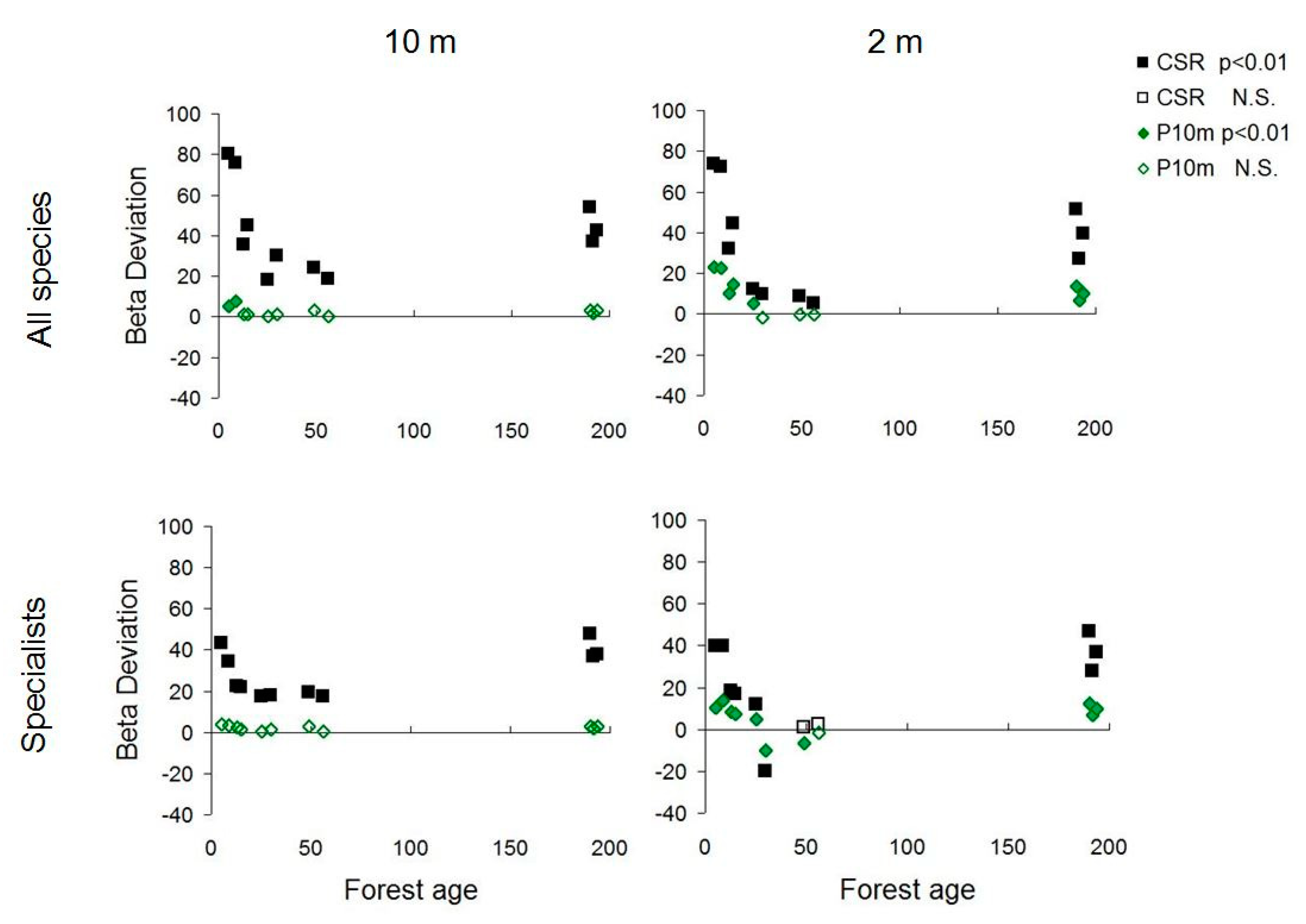
2.4. Null Models and Statistical Analyses

Two types of null models were generated by computer using Monte Carlo randomizations. First, to remove the effect of alpha diversity from beta diversity estimates (cf. [35,54]), we randomized the position of presences of species along the transect maintaining the same frequencies as in the field (CSR = complete spatial randomness). CSR removed all spatial autocorrelations and associations. Therefore, the remaining patterns were driven only by species abundances and species richness. Second, we applied spatially restricted randomizations (a discrete version of inhomogeneous Poisson process) where we randomized the positions of species presences within a particular interval using frequencies of species that appeared in this restricted part of the transect (Patch model, [55]). Patch model removed only fine scale autocorrelations and associations and maintained coarser scale spatial structures. For parametrizing the Patch model, we explored a series of interval sizes from 2 m to 20 m. However, we present here only the most relevant results with the 10 m interval size (referred as P10m). Independent simulations numbering 999 were used to assess the distributions of each randomized models.

As the distributions of randomized data might differ from normal distributions, the standard effect sizes were expressed by non-parametric measures,

SES CD = (CD_obs − median CD_rand)/(Q3 CD_rand − Q1 CD_rand)

Beta deviation = (BC_obs − median BC_rand)/(Q3 BC_rand − Q1 BC_rand)

where CD is the Compositional Diversity and BC is the Bray–Curtis dissimilarity, obs = observed data, rand = randomized data.

Overall trends of diversity measures were explored by linear and quadratic regressions. Alpha and beta diversity measures between stages of succession were compared by a nonparametric test (Kruskal–Wallis rank-test) for the several samples.

JNP-model 2.0 software [48] was used to perform the computerized sampling and the related analyses including randomization tests. Multivariate dissimilarity indices were calculated by the SYN-TAX 5.0 software package [56]. Differences between sites were analyzed using one-way ANOVA (with the three sites as levels) and with post hoc tests using LSD statistics [57]. In order to evaluate the difference in variance and possible trends among sites, the homogeneity of variance was tested by Levene statistics for each pair of sites [58]. Tests were performed with the PAST software [59].

3. Results

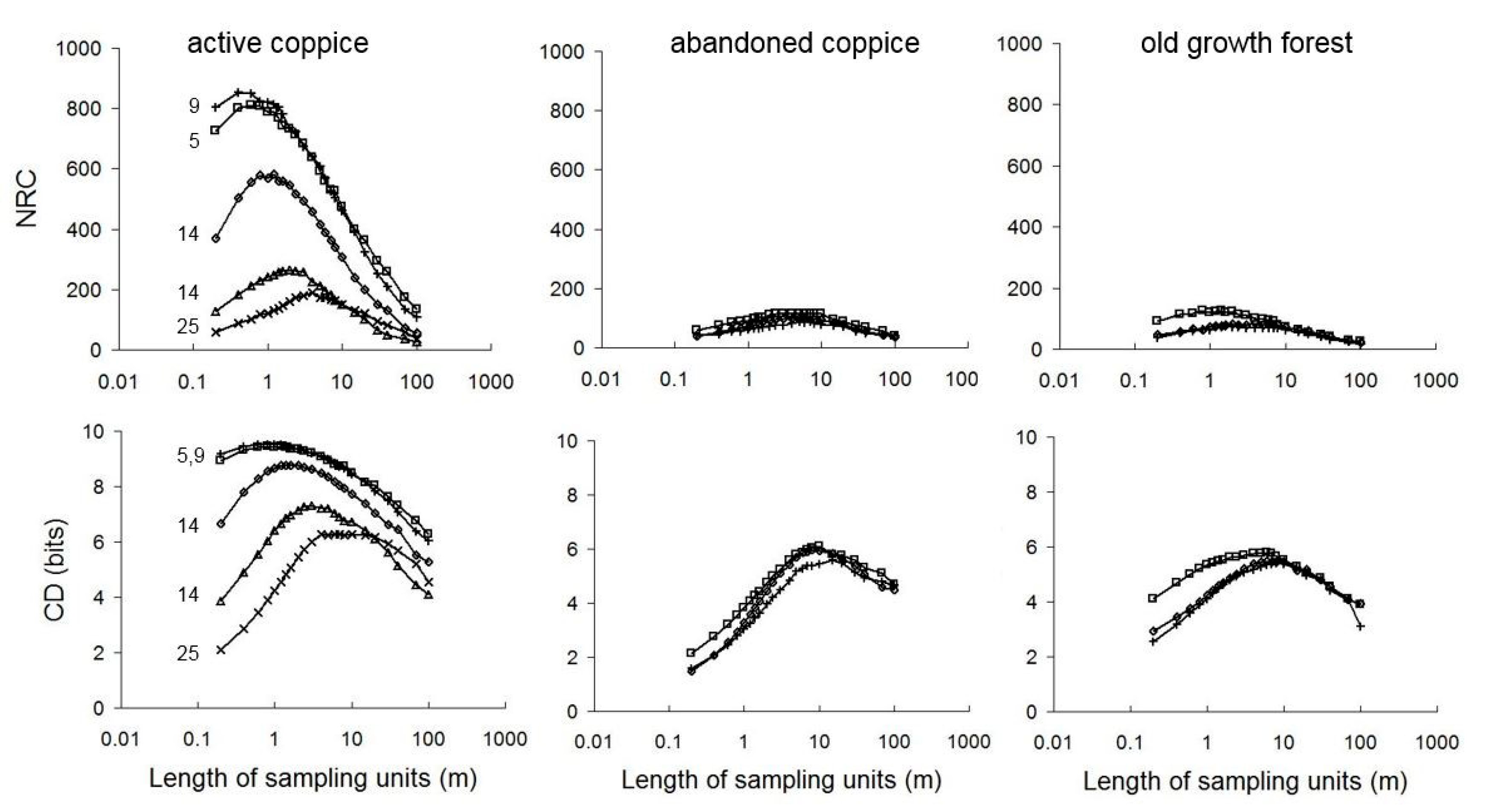
3.1. Scale Dependence of Diversity Patterns

The total number of species recorded along transects varied considerable between 121 (in active coppice stands) and 15 (in old-growth forests) showing a decreasing trend (Table 1). Beta diversity was a function of spatial resolution (sample grain) (Figure 1). The number and diversity of species combinations (NRC and CD) showed unimodal curves of variable shapes (Figure 1). The maximum number of realized species combinations varied between 852 and 189 in active coppice stands. Lower values between 76 and 125 were detected in abandoned coppice stands and in old growth forests (Figure 1). Maxima of these curves showed an overall decreasing trend in succession and shifted from finer to coarser scales. Based on these results, we selected two representative scales (i.e., 2 m and 10 m) for detailed studies (with various alpha and beta diversity indices).

At the 2 m scale, the largest mean species richness (6.99) appeared in active coppice stands, the smallest value (1.25) in abandoned coppice stands, while mean species richness was 2.08 in old-growth forests (

Table 2. Medians and ranges (in parentheses) of estimated diversity characteristics in the successional stages (all species considered). Significant differences between stages were evaluated by the Kruskall–Wallis non-parametric rank test and indicated by letters (p < 0.05 Bonferroni adjusted post-hoc tests).

	Alpha Diversity			Beta Diversity
	Species Richness	Shannon Diversity (bits)	Simpson Diversity	Patterns of Realized Species Combinations		Pairwise Spatial Dissimilarity			Spatial Variability Coefficient (CV %)
				NRC	CD (bits)	Sorensen	Bray–Curtis	Jaccard	Species Richness	Shannon Diversity	Simpson Diversity
(a) Scale: 10 m
Active coppice	18.350 A (27.050)	3.394 A (2.318)	0.853 A (0.308)	306 A (324)	7.718 A (1.353)	0.486 A (0.255)	60.060 A (20.524)	0.641 A (0.197)	28.743 A (31.293)	15.617 A (43.075)	7.769 A (44.221)
Abandoned coppice	3.950 B (0.950)	1.472 B (0.333)	0.533 B (0.086)	96 B (33)	5.925 B (0.172)	0.749 B (0.001)	82.201 B (2.774)	0.837 B (0.011)	68.463 B (13.368)	61.493 B (17.815)	53.378 B (21.371)
Old-growth	4.250 AB (1.950)	1.469 B (0.558)	0.537 AB (0.170)	71 B (10)	5.441 B (0.115)	0.477 AB (0.141)	53.958 AB (13.553)	0.630 AB (0.216)	41.021 AB (8.514)	43.556 AB (13.084)	40.896 C (22.206)
(b) Scale: 2 m
Active coppice	6.990 A (12.940)	2.314 A (2.750)	0.725 A (0.610)	545 A (575)	8.767 A (3.909)	0.713 A (0.227)	76.029 A (20.754)	0.806 A (0.111)	47.054 A (40.388)	33.208 A (99.888)	23.732 A (105.312)
Abandoned coppice	1.250 B (0.270)	0.380 B (0.130)	0.157 B (0.044)	90 B (40)	4.439 B (0.804)	0.811 A (0.024)	83.095 A (2.008)	0.830 A (0.0279)	107.422 B (10.076)	173.172 B (21.696	163.104 B (24.413)
Old-growth	2.080 AB (1.490)	0.737 AB (0.607)	0.308 AB (0.201)	81 B (49)	4.873 AB (0.809)	0.615 A (0.152)	66.943 A (13.223)	0.710 A (0.108)	62.266 AB (16.242	90.226 AB (44.04)	86.027 AB (47.705)

). A similar pattern was found at the 10 m scale where mean species richness varied between 18.35 (active coppice), 3.95 (abandoned coppice), and 4.25 (old-growth forest). In both cases, significant differences were found only between active and abandoned coppices.

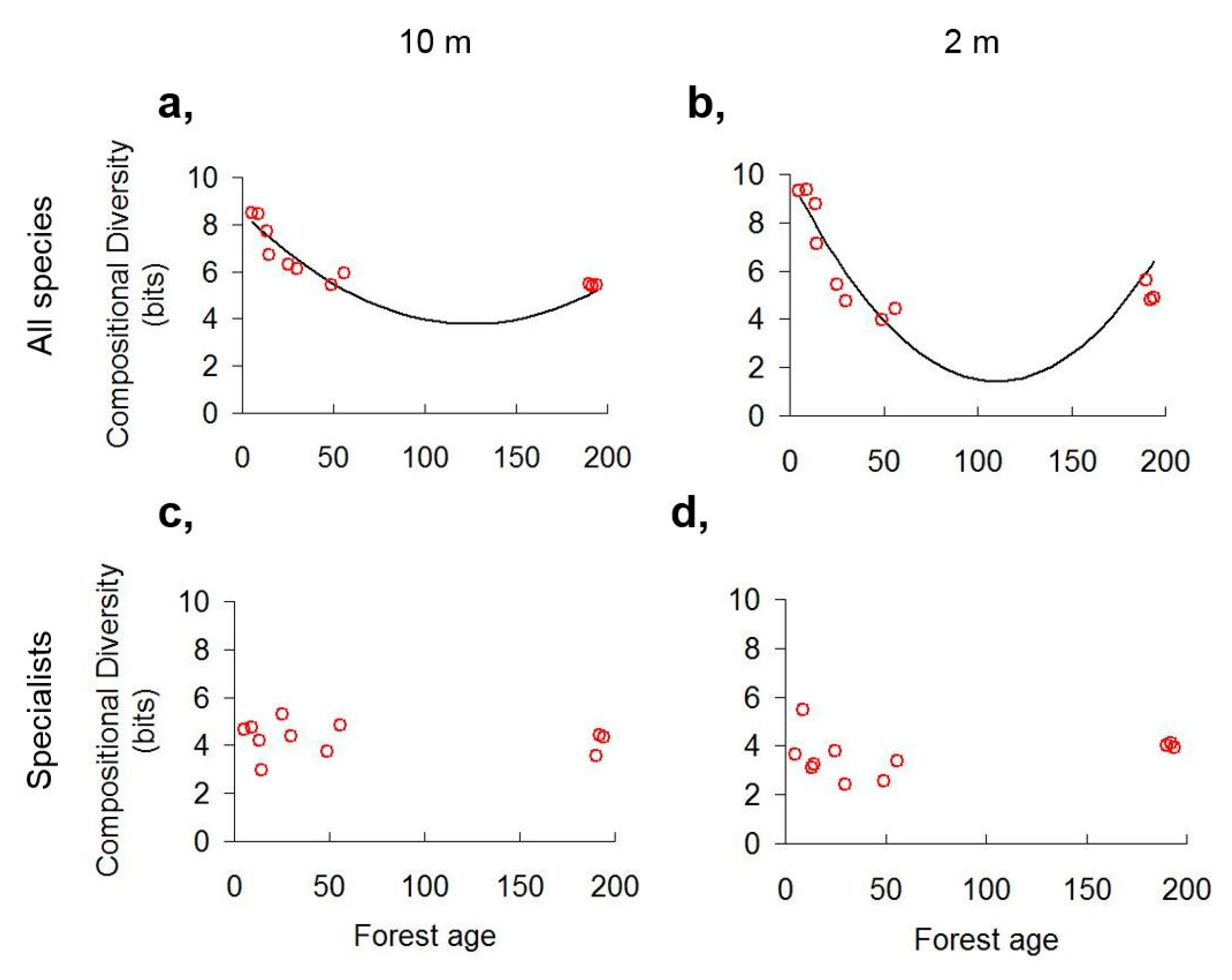
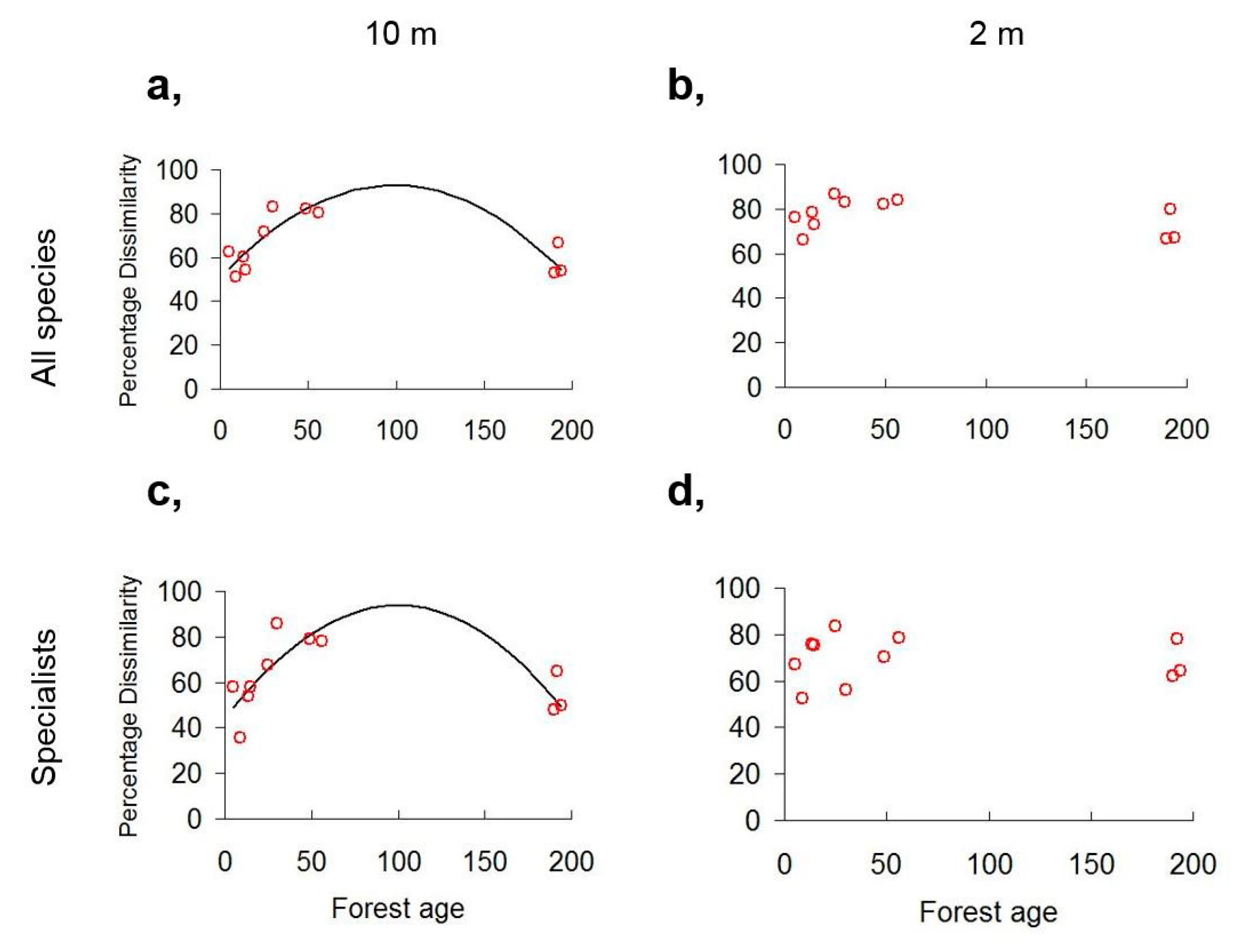
3.2. Diversity Trends along the Chronosequence

When all species had been considered, the quadratic model with U-shaped trend fitted best to the successional pattern of compositional diversity (Figure 2a,b). Bray–Curtis percentage dissimilarity showed an opposite humped back pattern (Figure 3a). These community level trends (with all species) were significant (p < 0.001) at 2 m and 10 m scales for compositional diversity and at 10 m scale (p < 0.05) for Bray–Curtis percentage dissimilarity (See Table S2).

Compositional diversity of beech forest specialists did not differ between stands along succession (Figure 2c,d) and Bray–Curtis percentage dissimilarity showed a significant trend (p < 0.05) only at the 10 m scale (Figure 3c,d).

Null models (i.e., removing spatial autocorrelations and interspecific associations by randomizations) resulted in similar unimodal beta diversity trends along the chronosequence (Figure S3). It suggests that changing species richness and abundance distributions drive these patterns. Beta deviation of Bray–Curtis dissimilarity showed U-shaped patterns along the chronosequence (Figure 4). Applying spatially restricted randomization within 10 m (Patch model), the U shape trend became weak at 2 m and almost completely disappeared at the 10 m scale. Beta diversity trends of compositional diversity also changed after randomizations. Standard effect size of compositional diversity varied between scales and data types (all species versus specialists) indicating varying degree of limitations to local coexistence relationships along the chronosequence (Figure 5).

3.3. Management Types and the Response of Beech Forest Specialists

When successional stages were compared, non-parametric tests showed significant differences between active and abandoned coppices at the 10 m scale (with smaller alpha diversity and diversity of species combinations and larger pairwise dissimilarity and larger spatial CV% in abandoned coppices) (Table 2). The diversity characteristics in old-growth stands showed intermediate values. Most diversity characteristics were similar between successional stages when beech forest specialists were tested separately (

Table 3. Medians and ranges of estimated diversity characteristics of beech forest specialists in the successional stages. Significant differences between stages were evaluated by the Kruskall–Wallis non-parametric rank test and indicated by letters (p < 0.05 Bonferroni adjusted post-hoc tests).

	Alpha Diversity			Beta Diversity
	Species Richness	Shannon Diversity (Bits)	Simpson Diversity	Patterns of Realized Species Combinations		Pairwise Spatial Dissimilarity			Spatial Variability Coefficient (CV%)
				NRC	CD (bits)	Sorensen	Bray–Curtis	Jaccard	Species Richness	Shannon Diversity	Simpson Diversity
(a) Scale: 10 m
Active coppice	3.350 A (3.800)	0.940 A (1.335)	0.393 A (0.413)	37 A (58)	4.667 A (2.361)	0.459 A (0.372)	57.777 A (31.86)	0.596 A (0.359)	39.164 A (30.835)	59.914 A (54.178)	54.333 A (60.752)
Abandoned coppice	1.950 B (0.750)	0.648 A (0.336)	0.270 A (0.120)	36 A (10)	4.369 A (1.056)	0.686 B (0.100)	78.055 B (6.919)	0.775 B (0.080)	68.891 B (17.298)	90.018 A (40.122)	88.557 A (37.881)
Old-growth	3.400 AB (0.650)	1.270 A (0.323)	0.489 A (0.133)	35 A (18)	4.354 A (0.858)	0.382 AB (0.174)	49.771 AB (16.854)	0.527 AB (0.187)	29.879 AB (6.917)	45.648 A (21.315)	43.642 A (28.545)
(b) Scale: 2 m
Active coppice	1.280 A (2.820)	0.319 A (1.346)	0.142 A (0.495)	40 A (88)	3.674 A (2.399)	0.663 A (0.417)	75.258 A (31.156)	0.717 A (0.293)	76.602 A (46.332)	153.399 A (149.210)	152.295 A (166.705)
Abandoned coppice	0.700 B (0.440)	0.148 A (0.130)	0.066 A (0.056)	23 A (21)	2.405 A (0.956)	0.673 A (0.201)	70.326 A (22.227)	0.830 A (0.214)	120.980 B (46.901)	272.111 B (119.666)	269.145 B (126.701)
Old-growth	1.720 AB (0.650)	0.584 A (0.352)	0.251 A (0.135)	37 A (7)	4.007 A (0.185)	0.564 A (0.192)	64.338 A (16.036)	0.656 A (0.150)	51.659 AB (23.020)	97.897 AB (48.175)	96.050 AB (47.758)

). Some tests showed the highest beta diversity in abandoned coppices but these patterns were inconsistent between scales and indices.

4. Discussion

In this paper we explored alpha and beta diversity patterns in the understory layer of sub-Mediterranean mountain beech forests. Our results support the U-shaped biodiversity model of forest succession. We found additional evidences for decreasing alpha diversity and novel evidences for decreasing true beta diversity during the first 60 years of succession after the last logging event. Beta diversity was scale dependent with a gradual shift of maximum compositional variability from fine (ca. 2 m) to coarser (ca. 10 m) scales within the coppice cycle. A characteristic 10 m spatial grain size emerged during the forest recovery process and it remained invariant in later successional stages.

4.1. Scale Dependence of Diversity Patterns

Beta diversity decreased with increasing sampling unit size (from 2 m to 10 m) and the difference was larger in active coppice stands than in older successional stands. These results support our first hypothesis (H1) and are in line with other studies [23,33]. In addition to the negative beta diversity–plot size relationship at scales larger than 2 m, we found an opposite positive beta diversity–plot size relationship at finer grains (between 0.2 m and 2 m). Other multi-scale studies exploring only coarser scales, could not detect this relationship as most forest studies used larger plot sizes (i.e., 100 m², 400 m² or 625 m²). Smaller plot sizes (<2 m²) were applied only exceptionally, see [9,17,21,26,37].

Considering the whole range of scales explored in our study from very fine (0.2 m) to coarse (100 m) resolutions, beta diversity followed unimodal curves. In our own previous studies using the same methodology, we found similar patterns [25,42,60]. However, to our knowledge, there are no other studies reporting this type of unimodal relationship between sampling unit size and beta diversity in forests.

The maximum of these curves (i.e., characteristic maximum scales, [30,44]) changed along the forest succession. Older stands had larger characteristic grain sizes according to the theory predicting increased complexity and mosaic diversity in old-growth natural forests. Few case studies assessed spatial scales explicitly. Comparing natural (pristine) forests with adjacent secondary forests, Campetella et al. [25] described a similar relationship with larger characteristic scales in pristine forest stands. Scheller and Mladenoff [61] reported an opposite trend with a 70 m characteristic scale (assessed by geostatistics) in secondary forests, and finer 20 m grain size in old-growth forests. Although the relationship was opposite, it is important to note that the 20 m characteristic scale estimated in old-growth forests by Scheller and Mladenoff [61] was close to the 10 m characteristic scale estimated in our study. The similar magnitude of scales might reflect similar pattern generating processes, i.e., it probably reflects variability in the structure of forest canopy.

4.2. Diversity Trends in Forest Succession

Our sampling design was optimized for assessing beta diversity, cf. [34]. However, the 200 m long transects were appropriate also for estimating the mean and spatial variation of alpha diversity. Using traditional 20 m × 20 m plots for assessing the successional pattern of species richness in the same area (in more stands at landscape scale), Bartha et al. [2] found the same trend and similar magnitudes of alpha diversity. We found larger alpha diversity in active coppice compared to abandoned coppice stands. Our results are in line with other studies that reported decreasing of alpha diversity between early and middle stages of forest succession [8,10]. The lowest alpha diversity appeared in middle stages of succession (i.e., abandoned coppice stands). Active coppice stands showed significantly higher values, while alpha diversity in old-growth forests was intermediate. This trend of alpha diversity in succession is consistent with the U-shaped diversity model [6,20] and supports our 2nd hypothesis (H2).

Patterns of beta diversity indices along the chronosequence showed also a quadratic (unimodal) relationship. Consistent with the U-shaped diversity model, beta diversity indices based on the spatial variability of species combinations (NRC and CD) had minimum values in the middle stages of forest succession. In contrast, other families of traditional beta diversity indices (expressed by the spatial dissimilarity of species combinations or by the standardized variance of alpha diversity) had maximum values in the middle stages of succession, i.e., followed a humped-back model. These opposite patterns can be explained by the inherent relationships between alpha diversity and most beta diversity indices [54].

Beta diversity indices which are positively correlated to alpha diversity (NRC and CD, cf. [62]) showed the same U-shaped trends as alpha diversity. Sorensen, Bray–Curtis, and Jaccard dissimilarity indices and the CV% of alpha diversity measures which all have negative correlations with alpha diversity [35,54] showed the opposite humped-back patterns. After removing the confounding effect of alpha diversity, these humped-back patterns turned also to U-shaped patterns. Therefore, we found strong evidences that true beta diversity (i.e., independently from alpha diversity, due to the use of null models) can be described also by the U-shaped diversity model in succession, similar to alpha diversity. We emphasize two different aspects of beta diversity. The original indices (cf. Figure 2 and Figure 3) reflect spatial variability. In contrast, the transformed beta diversity estimates (Beta deviation and SES of CD, cf. Figure 4 and Figure 5) reflect significant deviation from null models and only these versions are true measures of spatial heterogeneity. These measures showed the highest heterogeneity in early succession and in late succession (that is the U-shape), with slightly higher values in active coppice stands.

4.3. Assembly Processes Inferred from Diversity Patterns

In this study, more than 800 different species combinations were found at the 1 m scale in active coppices. This number decreased to ca. 200 species combinations by the end of the coppice cycle (within 25 years). In later successional stages the number of realized species combinations decreased further by another 50% and varied between 76 and 125 combinations. To our knowledge, this is a unique study reporting such complexity of realized coexistence relations of vascular understory species in forest succession. For assessing constraints on coexistence (i.e., assembly rules) differences between observed and expected species combinations need to be estimated. Biased estimates (due to small sample sizes), might prevent the detection of significant assembly rules.

We found significant differences between observed and expected species combinations in all stages of forest succession. Standard effect sizes were smaller at the 10 m scale and decreased with stand age. A similar trend was described by Zobel et al. [19] who studied a 250 year chronosequence from clear-cut to regenerated steady-state forest. In our study, effect sizes changed also between null models. The large deviations from the completely randomized patterns became minor or non-significant when the Patch model was used. It implies that most of the spatial heterogeneity appeared at scales larger than 10 m and might have been driven by the heterogeneity of tree canopy.

Comparing the large number of potential drivers of understory species composition in old-growth forests in Southern Europe, Sabatini et al. [13] found light availability and fine scale soil attributes as best predictors of compositional variability, while dispersal limitation had a minor role in structuring understory vegetation. Similar results were reported by other studies [9,20,33,36,63]. Comparing the spatial patterns of light and understory species, Tinya and Ódor [64] identified two characteristic scales in light patterns: 10 × 10 m grain size reflected small openings in the canopy (imperfect insertions) and 25 × 25 m reflected larger gaps due to treefalls. Tree seedlings correlated with the coarser 25 × 25 m scale and herbs and bryophytes with the finer 10 × 10 m scale. In our study, we also identified a characteristic 10 m scale that reflected the maximum variability of understory species composition, that probably is driven by light patterns. The finer 2 m characteristic scale we found in early stage of succession was transitional (characteristic between year 5 and 14 only) and probably driven by the spatial patterns of shrubs and the architecture of clonal herbs [40].

4.4. Patterns of Beech Forest Specialists and Management Implications

Timber harvest is the most challenging period in managed forests [2,28]. Species adapted to permanent forest canopy can be lost due to disturbances and stresses associated with logging. Recovery of this valuable group of species is usually slow and incomplete in most human modified landscape after clear-cuts [21,65].

In contrast to studies reporting succession after clear-cut logging, we did not find significant collapse of the alpha and beta diversity of beech forest specialists after coppicing with standards. We should reject our 3rd hypothesis (H3) because alpha and beta diversities of specialists were similar along the chronosequence. Figure S4 shows similar spatial patterns of beech forest specialists between successional stages (except for abandoned coppice), while the spatial patterns of forest generalists and other species (open habitat, forest edge and weedy species) expressed considerable changes. The increased Bray–Curtis dissimilarity of specialists at 10 m scale and the increased spatial CV% of alpha diversities at 2 m can be interpreted as a rarity driven (total abundance and alpha diversity driven) response of beta diversity to the closing tree canopy in abandoned coppices [36]. The significant spatial heterogeneity of specialists detected by null models can be interpreted by the associations of specialists to microhabitats heterogeneity. The typical U-shaped patterns of Beta deviation reflect temporally decreased (but still significant) heterogeneity in middle succession. The high beta diversity found in our study suggests a high number of available microhabitats linked to coppice with standards management. While diversity of generalists and other species underwent very strong changes, the contribution of specialists did not change.

These results provide further evidence about the positive role of traditional coppicing [8,27,29] and underline the need to preserve or reintroduce this type of management.

4.5. Beta Diversity as Indicator of Coexistence Relationships in Forest Understory

Forests are characterized by complex and dynamic mosaic structures [16,63]. Our results confirm previous suggestions that beta diversity indices are better indicators of forest understory diversity than the more widespread alpha diversity indices [13,16,17,25,60]. It has been generally accepted that assessing beta diversity needs a multi-scale approach [17,25,31,42]. In addition to previous experiences, the present study demonstrated the importance of using very large sample sizes (1,000 units or more), detailed spatial scaling (where the sample unit sizes are increased in small steps), and the inclusion of the rarely explored domain of scales between 0.2 m and 2 m. In line with Mori et al [36], our study confirmed the need to use several null models. Our sampling design (long transects of contiguous small plots) was appropriate to satisfy all of these criteria, therefore we propose it for future complex assessments.

For testing specific questions, simple indicators of beta diversity can be appropriate as well. According to our results, the standardized spatial variability coefficients (e.g., CV% of alpha diversity; [17,26,50]) can be recommended in this case.

5. Conclusions

Our study supported the recently proposed U-shaped alpha diversity model. In addition, we found novel evidence for a similar U-shaped beta diversity model in forest succession. We conclude that high resolution and high extent sampling in the field, together with the use of several indices with null models and detailed spatial scaling in analyses are required for precise and reliable estimation of forest understory beta diversity.

Our results highlight the importance of traditional coppice management in diversity maintenance. In contrast to expectation, we presented evidences that diversity of forest specialists might increase shortly after the coppicing events and that it is maintained over the rotation cycles. To further explore the functional role of beta diversity in these systems, future studies should focus on the spatial associations between beech forest specialists and the particular microhabitats.

References

1. Gilliam, F.S. The ecological significance of the herbaceous layer in temperate forest ecosystems. BioScience 2007, 57, 845–857. [Google Scholar] [CrossRef]
2. Bartha, S.; Merolli, A.; Campetella, G.; Canullo, R. Changes of vascular plant diversity along a chronosequence of beech coppice stands, central Apennines, Italy. Plant Biosyst. 2008, 142, 572–583. [Google Scholar] [CrossRef]
3. Canullo, R.; Simonetti, E.; Cervellini, M.; Chelli, S.; Bartha, S.; Wellstein, C.; Campetella, G. Unravelling mechanisms of short-term vegetation dynamics in complex coppice forest systems. Folia Geobot. 2017, 52, 71–81. [Google Scholar] [CrossRef]
4. Horn, H. The ecology of secondary succession. Ann. Rev. Ecol. Syst. 1974, 5, 25–37. [Google Scholar] [CrossRef]
5. Christensen, N.L.; Peet, R.K. Convergence during Secondary Forest Succession. J. Ecol. 1984, 72, 25–36. [Google Scholar] [CrossRef]
6. Jules, M.J.; Sawyer, J.O.; Jules, E.S. Assessing the relationships between stand development and understory vegetation using a 420-year chronosequence. For. Ecol. Manag. 2008, 155, 2384–2393. [Google Scholar] [CrossRef]
7. Kirby, K.J.; Thomas, R.C. Changes in the ground flora in Wytham Woods, southern England from 1974 to 1991—Implications for nature conservation. J. Veg. Sci. 2000, 11, 871–880. [Google Scholar] [CrossRef]
8. Müllerová, J.; Hédl, R.; Szabó, P. Coppice abandonment and its implications for species diversity in forest vegetation. For. Ecol. Manag. 2015, 343, 88–100. [Google Scholar] [CrossRef] [Green Version]
9. Ujházy, K.; Hederová, L.; Máliš, F.; Ujházyová, M.; Bosela, M.; Čiliak, M. Overstorey dynamics controls plant diversity in age-class temperate forests. For. Ecol. Manag. 2017, 391, 96–105. [Google Scholar] [CrossRef]
10. Della Longa, G.; Boscutti, F.; Marini, L.; Alberti, G. Coppicing and plant diversity in a lowland wood remnant in North–East Italy. Plant Biosyst. 2019. [Google Scholar] [CrossRef]
11. Balvanera, P.; Lott, E.; Gerardo, S.; Siebe, C.; Islas, A. Patterns of beta-diversity in a Mexican tropical dry forest. J. Veg. Sci. 2002, 13, 145–158. [Google Scholar] [CrossRef]
12. Campetella, G.; Botta-Dukát, Z.; Wellstein, C.; Canullo, R.; Gatto, S.; Chelli, S.; Mucina, L.; Bartha, S. Patterns of plant trait–environment relationships along a forest succession chronosequence. Agric. Ecosyst. Environ. 2011, 145, 38–48. [Google Scholar] [CrossRef]
13. Sabatini, F.M.; Burrascano, S.; Tuomisto, H.; Blasi, C. Ground Layer Plant Species Turnover and Beta Diversity in Southern-European Old-Growth Forests. PLoS ONE 2014, 9, e95244. [Google Scholar] [CrossRef]
14. Ottaviani, G.; Götzenberger, L.; Bacaro, G.; Chiarucci, A.; de Bello, F.; Marcantonio, M. A multifaceted approach for beech forest conservation: Environmental drivers of understory plant diversity. Flora 2019, 256, 85–91. [Google Scholar] [CrossRef]
15. Qian, H.; Klinka, K.; Sivak, B. Diversity of the understorey vascular vegetation in 40 year-old and old-growth forest stands on Vancouver Island, British Columbia. J. Veg. Sci. 1997, 8, 773–780. [Google Scholar] [CrossRef]
16. Bobiec, A. The mosaic diversity of field layer vegetation in the natural and exploited forests of Bialowieza. Plant Ecol. 1998, 136, 175–187. [Google Scholar] [CrossRef] [Green Version]
17. Standovár, T.; Ódor, P.; Aszalós, R.; Gáhidy, L. Sensitivity of ground layer vegetation diversity descriptors in indicating forest naturalness. Commun. Ecol. 2006, 7, 199–209. [Google Scholar] [CrossRef] [Green Version]
18. Burrascano, S.; Rosati, L.; Blasi, C. Plant species diversity in Mediterranean old-growth forest: A case study from central Italy. Plant Biosyst. 2009, 143, 190–200. [Google Scholar] [CrossRef]
19. Zobel, K.; Zobel, M.; Peet, R.K. Changes in pattern diversity during secondary succession in Estonian forests. J. Veg. Sci. 1993, 4, 489–498. [Google Scholar] [CrossRef]
20. Hilmers, T.; Friess, N.; Bassler, C.; Heurich, M.; Brandl, R.; Pretzsh, H.; Seidl, R.; Müller, J. Biodiversity along temperate forest succession. J. Appl. Ecol. 2018, 55, 2756–2766. [Google Scholar] [CrossRef] [Green Version]
21. Moola, F.M.; Vasseur, L. Recovery of late-seral vascular plants in a chronosequence of post-clearcut forest stands in coastal Nova Scotia, Canada. Plant Ecol. 2004, 172, 183–197. [Google Scholar] [CrossRef]
22. Amici, V.; Santi, E.; Filibeck, G.; Diekmann, M.; Geri, F.; Landi, S.; Scoppola, A.; Chiarucci, A. Influence of secondary forest succession on plant diversity patterns in a Mediterranean landscape. J. Biogeogr. 2013, 40, 2335–2347. [Google Scholar] [CrossRef]
23. López-Martinez, J.O.; Hernández-Stefanoni, J.L.; Dupuy, J.M.; Meave, J.A. Partitioning the variation of woody plant β-diversity in a landscape of secondary tropical dry forests across spatial scales. J. Veg. Sci. 2013, 24, 33–45. [Google Scholar] [CrossRef]
24. Burrascano, S.; Ripullone, F.; Bernardo, L.; Borghetti, M.; Carli, E.; Colangelo, M.; Gangale, C.; Gargano, D.; Gentilesca, T.; Luzzi, G.; et al. It’s a long way to the top: Plant species diversity in the transition from managed to old-growth forests. J. Veg. Sci. 2018, 29, 98–109. [Google Scholar] [CrossRef] [Green Version]
25. Campetella, G.; Canullo, R.; Bartha, S. Coenostate descriptors and spatial dependence in vegetation: Derived variables in monitoring forest dynamics and assembly rules. Commun. Ecol. 2004, 5, 105–114. [Google Scholar] [CrossRef]
26. Moora, M.; Daniell, T.; Kalle, H.; Liira, J.; Püssa, K.; Roosaluste, E.; Öpik, M.; Wheatley, R.; Zobel, M. Spatial pattern and species richness of boreonemoral forest understorey and its determinants—A comparison of differently managed forests. For. Ecol. Manag. 2007, 250, 64–70. [Google Scholar] [CrossRef]
27. Decocq, G.; Aubert, M.; Dupont, F.; Alard, D.; Saguez, R.; Wattez-Franger, A.; De Fucault, B.; Delelis-Dusollier, A.; Bardat, J. Plant diversity in a managed temperate deciduous forest: Understorey response to two silvicultural systems. J. Appl. Ecol. 2004, 41, 1065–1079. [Google Scholar] [CrossRef]
28. Campetella, G.; Canullo, R.; Gimona, A.; Garadnai, J.; Chiarucci, A.; Giorgini, D.; Angelini, E.; Cervellini, M.; Chelli, S.; Bartha, S. Scale-dependent effects of coppicing on the species pool of late successional beech forests in the central Apennines, Italy. Appl. Veg. Sci. 2016, 19, 474–485. [Google Scholar] [CrossRef] [Green Version]
29. Cervellini, M.; Fiorini, S.; Cavicchi, A.; Campetella, G.; Simonetti, E.; Chelli, S.; Canullo, R.; Gimona, A. Relationships between understory specialist species and local management practices in coppiced forests—Evidence from the Italian Apennines. For. Ecol. Manag. 2017, 385, 35–45. [Google Scholar] [CrossRef]
30. Juhász-Nagy, P.; Podani, J. Information theory methods for the study of spatial processes and succession. Vegetatio 1983, 51, 129–140. [Google Scholar] [CrossRef]
31. Podani, J.; Czárán, T.; Bartha, S. Pattern, area and diversity: The importance of spatial scale in species assemblages. Abstr. Bot. 1993, 17, 37–51. [Google Scholar]
32. Anderson, M.J.; Crist, T.O.; Chase, J.M.; Vellend, M.; Inouye, B.D.; Freestone, A.L.; Sanders, N.J.; Cornell, H.V.; Comita, L.S.; Davies, K.F.; et al. Navigating the multiple meanings of diversity: A roadmap for the practicing ecologist. Ecol. Lett. 2011, 14, 19–28. [Google Scholar] [CrossRef] [PubMed]
33. Mi, X.; Swenson, N.G.; Jia, Q.; Rao, M.; Feng, G.; Ren, H.; Daniel, P.; Bebber, D.P.; Ma, K. Stochastic assembly in a subtropical forest chronosequence: Evidence from contrasting changes of species, phylogenetic and functional dissimilarity over succession. Sci. Rep. 2016, 6, 32596. [Google Scholar] [CrossRef]
34. Bartha, S.; Campatella, G.; Canullo, R.; Bódis, J.; Mucina, L. On the importance of fine-scale spatial complexity in vegetation restoration. Int. J. Ecol. Environ. Sci. 2004, 30, 101–116. [Google Scholar]
35. Chase, J.M.; Kraft, N.J.B.; Smith, K.G.; Vellend, M.; Inouye, B.D. Using null models to disentangle variation in community dissimilarity from variation in alpha-diversity. Ecosphere 2011, 2, 1–11. [Google Scholar] [CrossRef]
36. Mori, A.S.; Fujii, S.; Kitagawa, R.; Koide, D. Null model approaches to evaluating the relative role of different assembly processes in shaping ecological communities. Oecologia 2015, 178, 261–273. [Google Scholar] [CrossRef]
37. Ódor, P.; Standovár, T. Substrate specificity and community structure of bryophyte vegetation in a near-natural montane beech forest. Commun. Ecol. 2002, 3, 39–49. [Google Scholar] [CrossRef]
38. Piovesan, G.; Di Filippo, A.; Alessandrini, A.; Biondi, F.; Schirone, B. Structure, dynamics and dendroecology of an old-growth Fagus forest in the Apennines. J. Veg. Sci. 2004, 16, 13–28. [Google Scholar] [CrossRef]
39. Mucina, L.; Bültmann, H.; Dierßen, K.; Theurillat, J.-P.; Raus, T.; Čarni, A.; Šumberová, K.; Willner, W.; Dengler, J.; García, R.G.; et al. Vegetation of Europe: Hierarchical floristic classification system of vascular plant, bryophyte, lichen, and algal communities. Appl. Veg. Sci. 2016, 19, 3–264. [Google Scholar] [CrossRef]
40. Canullo, R.; Campetella, G.; Mucina, L.; Chelli, S.; Wellstein, C.; Bartha, S. Patterns of clonal growth modes along a chronosequence of post-coppice forest regeneration in beech forest of Central Italy. Folia Geobot. 2011, 46, 271–288. [Google Scholar] [CrossRef]
41. Pickett, S.T.A. Space-for-time substitution as an alternative to long-term studies. In Long-Term Studies in Ecology; Likens, G.E., Ed.; Springer: New York, NY, USA, 1989; pp. 110–135. [Google Scholar]
42. Campetella, G.; Canullo, R.; Bartha, S. Fine scale spatial pattern analysis of herb layer of woodland vegetation using information theory. Plant Biosyst. 1999, 133, 277–288. [Google Scholar] [CrossRef]
43. Podani, J. Computerized sampling in vegetation studies. Coenoses 1987, 2, 9–18. [Google Scholar]
44. Juhász-Nagy, P. On some ‘characteristic area’ of plant community stands. Proc. Colloq. Inf. Theor. 1967, 269–282. [Google Scholar]
45. Juhász-Nagy, P. Spatial dependence of plant populations. Part 1. Equivalence analysis (an outline for a new model). Acta Bot. Acad Sci. Hung 1976, 22, 61–78. [Google Scholar]
46. Juhász-Nagy, P. Notes on diversity. Part, I. Introduction. Abstr. Bot. 1984, 8, 43–55. [Google Scholar]
47. Juhász-Nagy, P. Spatial dependence of plant populations. Part 2. A family of new models. Acta Bot. Acad Sci. Hung 1984, 30, 363–402. [Google Scholar]
48. Bartha, S.; Czárán, T.; Podani, J. Exploring plant community dynamics in abstract coenostate spaces. Abstr. Bot. 1998, 22, 49–66. [Google Scholar]
49. Podani, J. Analysis of mapped and simulated vegetation patterns by means of computerized sampling techniques. Acta Bot. Hung 1984, 30, 403–425. [Google Scholar]
50. Bartha, S.; Campetella, G.; Kertész, M.; Hahn, I.; Kröel-Dulay, G.; Rédei, T.; Kun, A.; Virágh, K.; Fekete, G.; Kovács-Láng, E. Beta diversity and community differentiation in dry perennial sand grasslands. Ann. Bot. 2011, 1, 9–18. [Google Scholar]
51. Magurran, A. Measuring Biological Diversity; Blackwell Science Ltd.: Oxford, UK, 2004; p. 256. [Google Scholar]
52. Tuomisto, H. A diversity of beta diversities: Straightening up a concept gone awry. Part 2. Quantifying beta diversity and related phenomena. Ecography 2010, 33, 23–45. [Google Scholar] [CrossRef]
53. Podani, J. Introduction to the Exploration of Multivariate Biological Data; Backhuys Publishers: Leiden, The Netherlands, 2000; p. 407. [Google Scholar]
54. Jost, L. Partitioning diversity into independent alpha and beta components. Ecology 2007, 88, 2427–2439. [Google Scholar] [CrossRef] [PubMed] [Green Version]
55. Watkins, A.J.; Wilson, J.B. Fine-scale community structure of lawn. J. Ecol. 1992, 80, 15–24. [Google Scholar] [CrossRef]
56. Podani, J. SYN-TAXpc. Version 5.0. User’s Guide; Scientia Publishing: Budapest, Hungary, 1993. [Google Scholar]
57. Sokal, R.R.; Rohlf, F.J. Biometry: The Principles and Practice of Statistics in Biological Research, 3rd ed.; W.H. Freeman and Co.: New York, NY, USA, 1995. [Google Scholar]
58. Campbell, R.C. Statistics for Biologists, 2nd ed.; Cambridge University Press: Cambridge, UK, 1974. [Google Scholar]
59. Hammer, Ø.; Harper, D.A.T.; Ryan, P.D. PAST: Paleontological statistics software package for education and data analysis. Palaeontol. Electron. 2001, 4, 9. [Google Scholar]
60. Canullo, R.; Campetella, G. Spatial patterns of textural elements in a regenerative phase of a beech coppice (Torricchio Mountain Nature Reserve, Apennines, Italy). Acta Bot. Gall. 2005, 152, 529–543. [Google Scholar] [CrossRef] [Green Version]
61. Scheller, R.M.; Mladenoff, D.J. Understory species patterns and diversity in old-growth and managed Northern hardwood forests. Ecol. Appl. 2002, 12, 1329–1343. [Google Scholar] [CrossRef]
62. Bartha, S.; Collins, S.L.; Glenn, S.M.; Kertész, M. Fine-scale spatial organization of tallgrass prairie vegetation along a topographic gradient. Folia Geobot. Phytotax. 1995, 30, 169–184. [Google Scholar] [CrossRef]
63. Landuyt, D.; Perring, M.P.; Seidl, R.; Taubert, F.; Verbeeck, H.; Verheyen, K. Modelling understorey dynamics in temperate forests under global change–Challenges and perspectives. Perspect. Plant Ecol. 2018, 31, 44–54. [Google Scholar] [CrossRef] [Green Version]
64. Tinya, F.; Ódor, P. Congruence of the spatial pattern of light and understory vegetation in an old-growth, temperate mixed forest. For. Ecol. Manag. 2016, 381, 84–92. [Google Scholar] [CrossRef] [Green Version]
65. Godefroid, S.; Rucquoij, S.; Koedam, N. To what extent do forest herbs recover after clearcutting in beech forest? For. Ecol. Manag. 2005, 210, 39–53. [Google Scholar] [CrossRef]
Figure 1. Scale dependence of beta diversity in beech forests. Beta diversity (spatial variability of species composition) estimated by the number (NRC) and diversity (CD) of realized species combinations. Numbers refer to ages (years after the last logging event). Note that both NRC and CD are scale dependent and show unimodal patterns with the increasing length of sampling units. Based on the peaks of these curves we delineated two representative scales (2 m and 10 m) for further analyses.
Diversity 12 00101 g001
Figure 2. Beta diversity along the chronosequence represented by Compositional Diversity. Significant quadratic models are shown. (a) For all species at 10 m scale: Y = 0.0003 x2 − 0.0752 x + 8.4953 (R2 = 0.855 p < 0.001). (b) For all species at 2 m scale: Y = 0.0007 x2 − 0.1539 x + 9.892 (R2 = 0.8627 p < 0.001). (c,d) show non-significant relationships.
Diversity 12 00101 g002
Figure 3. Beta diversity along the chronosequence represented by Bray–Curtis Percentage Dissimilarity. Significant quadratic models are shown. (a) For all species at 10 m scale: Y = −0.0043 x2 + 0.8514 x + 50.780 (R2 = 0.7227 p < 0.05). (c) For specialists at 10 m scale: Y = −0.005 x2 − 0.998 x + 43.992 (R2 = 0.6257 p < 0.05). (b,d) show non-significant relationships.
Diversity 12 00101 g003
Figure 4. Null model-based beta diversity trends (Beta deviation of Bray–Curtis Dissimilarity) along the chronosequence. CSR = null model based on Complete Spatial Randomizations, P10m = Patch model randomization with 10 m diameter.
Diversity 12 00101 g004
Figure 5. Null model-based beta diversity trends along the chronosequence. Standard effect size of Compositional Diversity (SES of CD). CSR = null model based on Complete Spatial Randomizations, P10m = Patch model randomization with 10 m diameter.
Diversity 12 00101 g005