Simple Selection Procedure to Distinguish between Static and Flexible Loops


Abstract

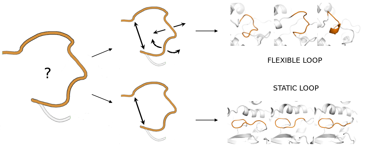
1. Introduction
2. Results
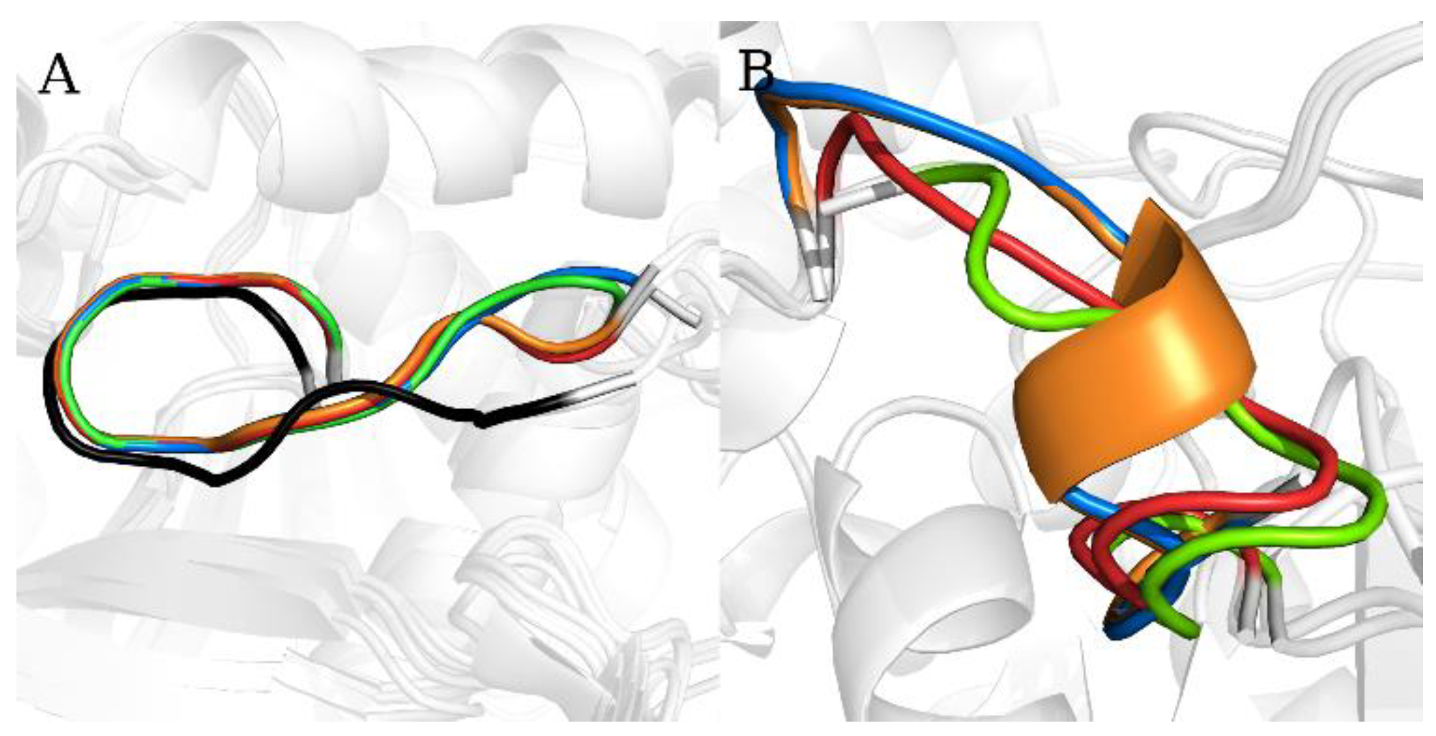
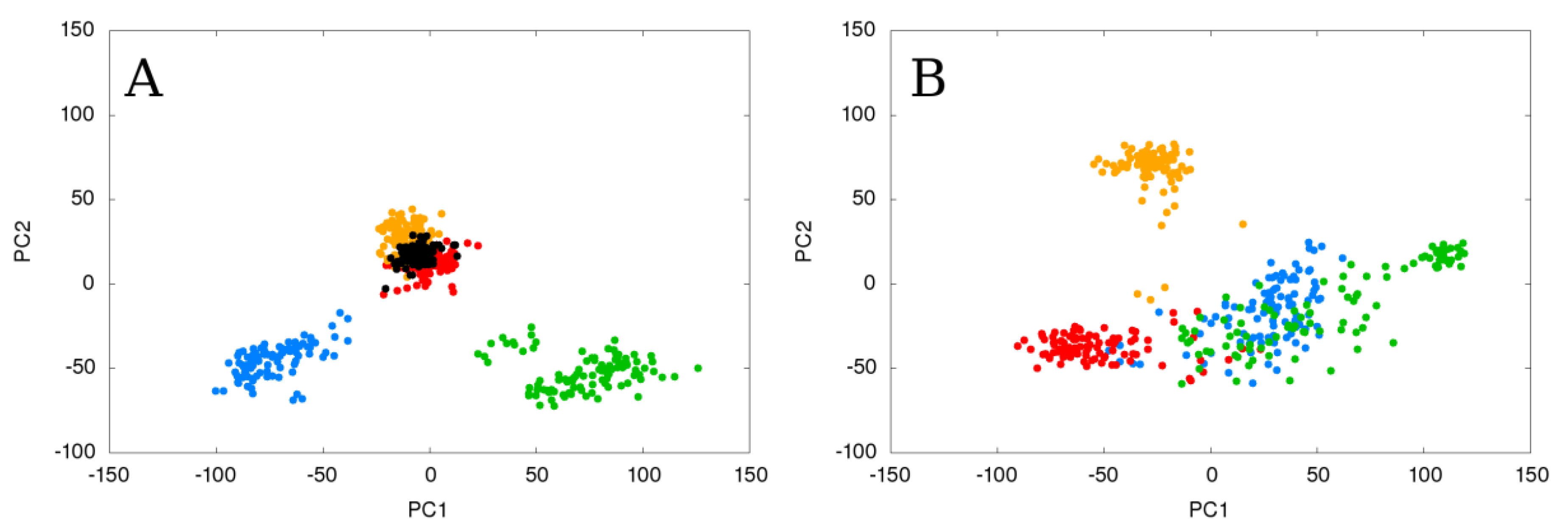
2.1. Static Loop Reconstruction
2.2. Flexible Loop Reconstruction
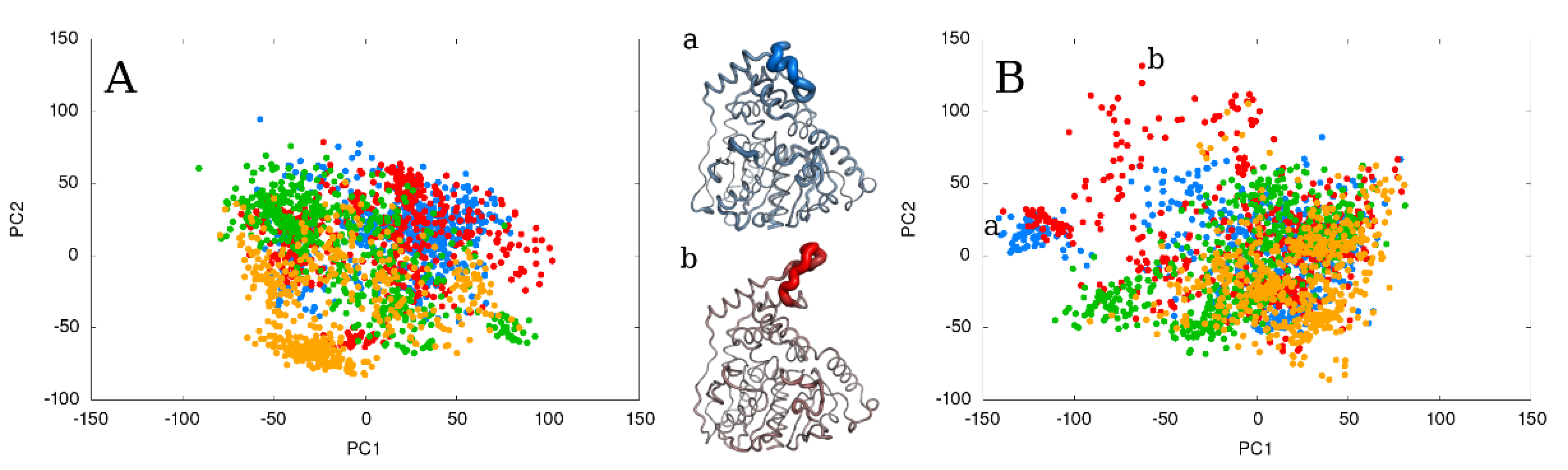
2.3. Flexible and Static Loops’ Comparison
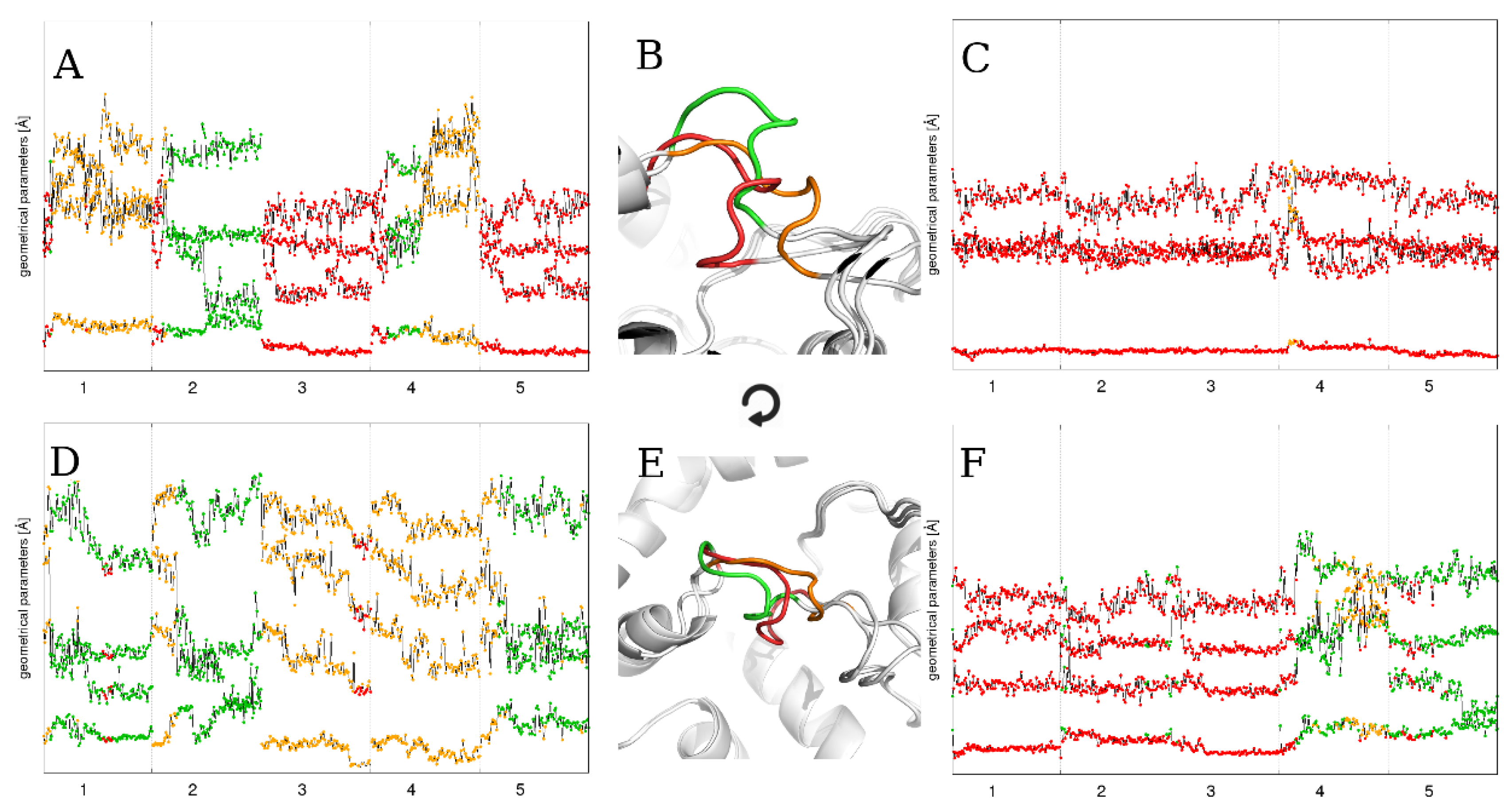
2.4. The Effect of Running Repetitions of Simulations
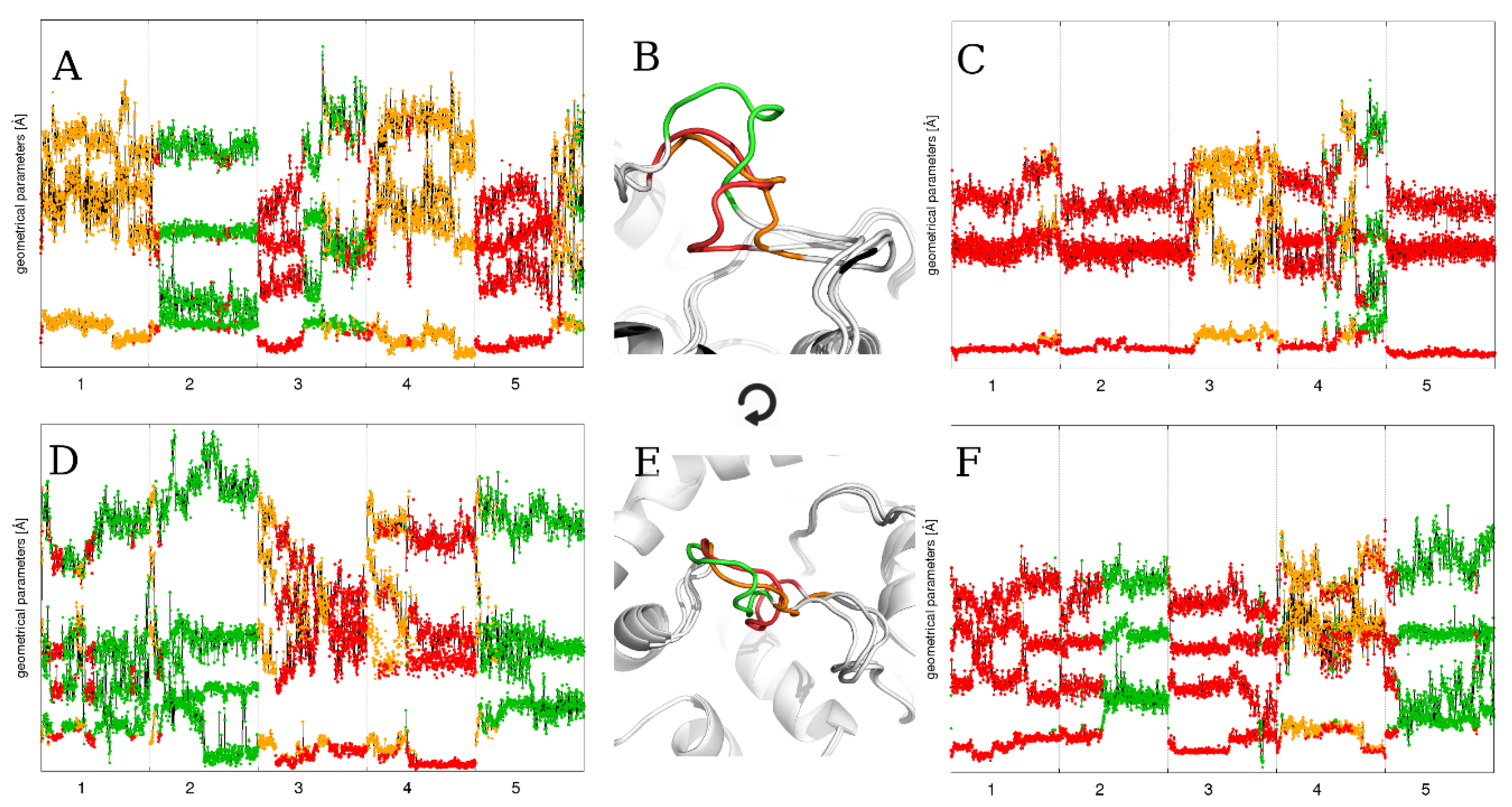
2.5. The Effect of Extending the Simulation Length
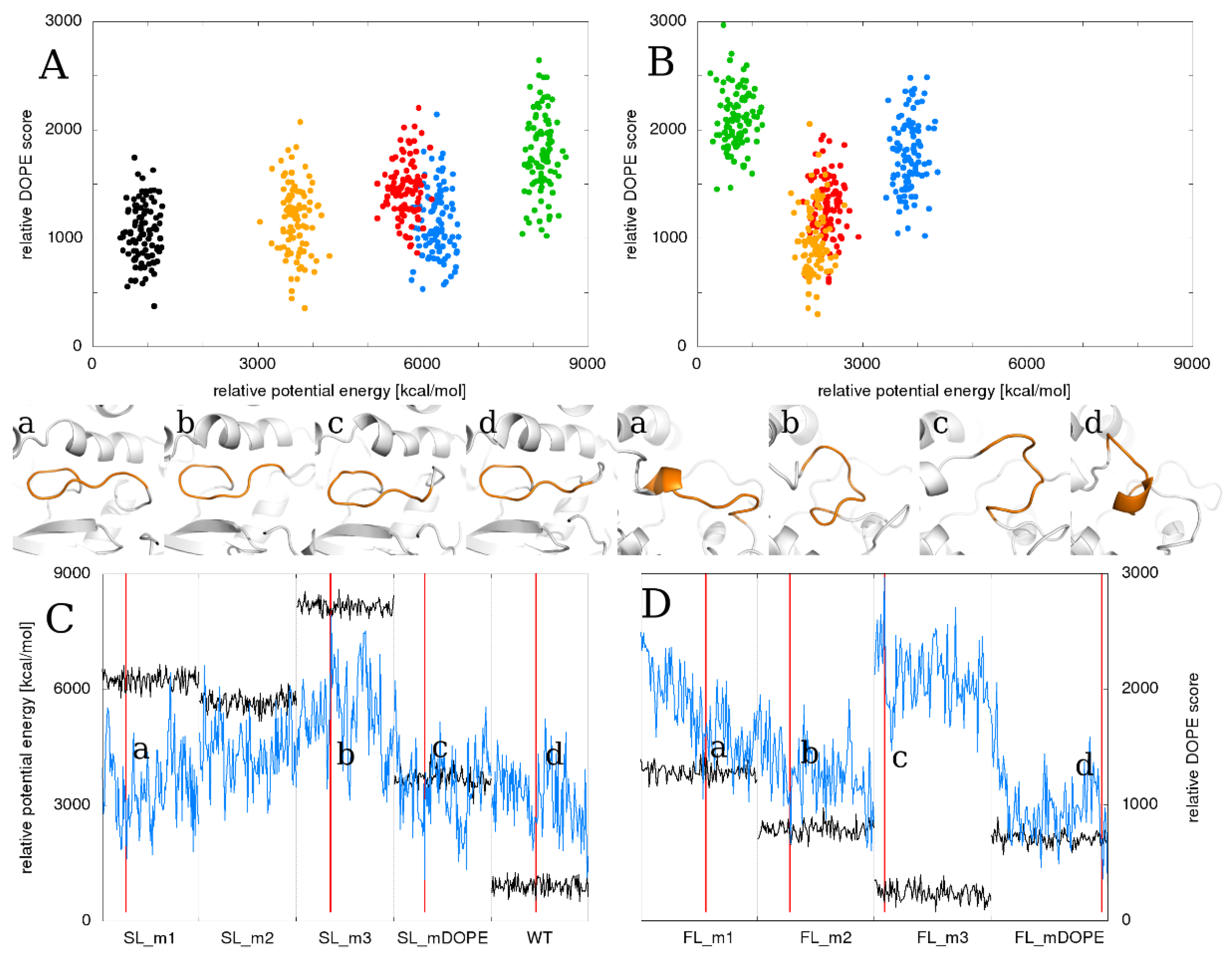
2.6. Relationship between the Total Energy and DOPE Score
3. Discussion
4. Materials and Methods
4.1. Loop Reconstruction
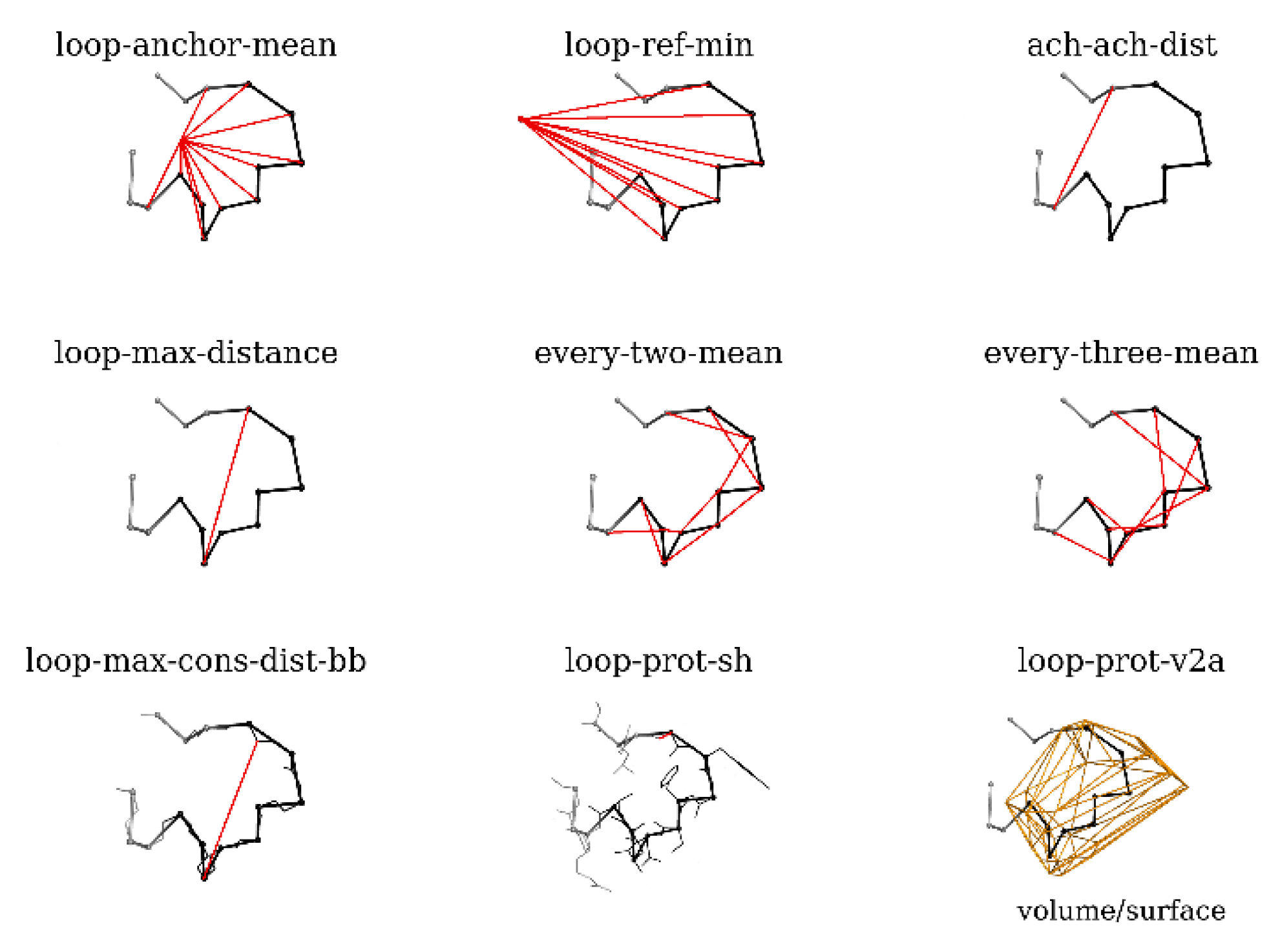
4.2. Model Selection
- -
- loop-anchor-mean: mean distance from the Cα atoms of loop residues and the centroid of the Cα atoms of the loop attachment points (residues 188 and 196 in BmJHEH and residues 318 and 326 in AnEH),
- -
- loop-ref-min: minimum distance from the Cα atoms of loop residues to the centroid of the Cα atoms of a conserved Trp residue located in the proximity of the active site in both structures (Trp154 in BmJHEH and Trp117 in AnEH),
- -
- ach-ach-dist: distance between the Cα atoms of the attachment points,
- -
- loop-max-distance: maximum distance between Cα atoms of the loop,
- -
- every-two-mean: mean value of the distance between Cα atoms of every second residue of the loop,
- -
- every-three-mean: mean value of the distance between Cα atoms of every third residue of the loop,
- -
- loop-max-cons-distance-bb: maximum distance between the loop backbone atoms (Cα, C and N),
- -
- loop-prot-sh: the minimum distance between the loop and protein (non-loop) atoms,
- -
- loop-prot-v2a: measure of loop sphericity; a ConvexHull approximation of the volume to area ratio of the loop.
4.3. Statistical Analysis of Loop Parameters
4.4. Molecular Dynamics Simulations and Normal Modes Analysis
5. Conclusions
Supplementary Materials
Author Contributions
Funding
Acknowledgments
Conflicts of Interest
Abbreviations
| AnEH | Aspergillus niger epoxide hydrolase |
| BmJHEH | Bombyx mori juvenile hormone epoxide hydrolase |
| SL | Static loop |
| FL | Flexible loop |
References
- Regad, L.; Martin, J.; Nuel, G.; Camproux, A.-C. Mining protein loops using a structural alphabet and statistical exceptionality. BMC Bioinform. 2010, 11, 75. [Google Scholar] [CrossRef]
- Gu, Y.; Li, D.-W.; Brüschweiler, R. Decoding the Mobility and Time Scales of Protein Loops. J. Chem. Theory Comput. 2015, 11, 1308–1314. [Google Scholar] [CrossRef]
- Fiser, A.; Sali, A. ModLoop: Automated modeling of loops in protein structures. Bioinformatics 2003, 19, 2500–2501. [Google Scholar] [CrossRef]
- Gora, A.; Brezovsky, J.; Damborsky, J. Gates of enzymes. Chem. Rev. 2013, 113, 5871–5923. [Google Scholar] [CrossRef]
- Espadaler, J.; Querol, E.; Aviles, F.X.; Oliva, B. Identification of function-associated loop motifs and application to protein function prediction. Bioinformatics 2006, 22, 2237–2243. [Google Scholar] [CrossRef]
- Uversky, V.N. Functional roles of transiently and intrinsically disordered regions within proteins. FEBS J. 2015, 282, 1182–1189. [Google Scholar] [CrossRef]
- Bala, S.; Shinya, S.; Srivastava, A.; Ishikawa, M.; Shimada, A.; Kobayashi, N.; Kojima, C.; Tama, F.; Miyashita, O.; Kohda, D. Crystal contact-free conformation of an intrinsically flexible loop in protein crystal: Tim21 as the case study. Biochim. Biophys. Acta 2020, 1864, 129418. [Google Scholar] [CrossRef]
- Au, D.F.; Ostrovsky, D.; Fu, R.; Vugmeyster, L. Solid-state NMR reveals a comprehensive view of the dynamics of the flexible, disordered N-terminal domain of amyloid-β fibrils. J. Biol. Chem. 2019, 294, 5840–5853. [Google Scholar] [CrossRef]
- Berman, H.M. The Protein Data Bank. Nucleic Acids Res. 2000, 28, 235–242. [Google Scholar] [CrossRef]
- Rose, P.W.; Prlić, A.; Altunkaya, A.; Bi, C.; Bradley, A.R.; Christie, C.H.; Di Costanzo, L.; Duarte, J.M.; Dutta, S.; Feng, Z.; et al. The RCSB protein data bank: Integrative view of protein, gene and 3D structural information. Nucleic Acids Res. 2017, 45. [Google Scholar] [CrossRef]
- Djinovic-Carugo, K.; Carugo, O. Missing strings of residues in protein crystal structures. Intrinsically Disord. Proteins 2015, 3, e1095697. [Google Scholar] [CrossRef]
- Panchenko, A.R.; Madej, T. Structural similarity of loops in protein families: Toward the understanding of protein evolution. BMC Evol. Biol. 2005, 5, 10. [Google Scholar] [CrossRef]
- Jacobson, M.; Sali, A. Comparative Protein Structure Modeling and its Applications to Drug Discovery. In Annual Reports in Medicinal Chemistry; Elsevier: Houston, TX, USA, 2004; pp. 259–276. ISBN 0120405393. [Google Scholar]
- Fiser, A. Template-Based Protein Structure Modeling. Methods Mol. Biol. 2010, 673, 73–94. [Google Scholar]
- Deng, H.; Jia, Y.; Zhang, Y. Protein structure prediction. Int. J. Mod. Phys. B 2018, 32, 1840009. [Google Scholar] [CrossRef]
- Lee, J.; Freddolino, P.L.; Zhang, Y. Ab Initio Protein Structure Prediction. In From Protein Structure to Function with Bioinformatics; Springer: Dordrecht, The Netherlands, 2017; pp. 3–35. ISBN 9789402410693. [Google Scholar]
- Park, H.; Lee, G.R.; Heo, L.; Seok, C. Protein Loop Modeling Using a New Hybrid Energy Function and Its Application to Modeling in Inaccurate Structural Environments. PLoS ONE 2014, 9, e113811. [Google Scholar] [CrossRef]
- Karami, Y.; Rey, J.; Postic, G.; Murail, S.; Tufféry, P.; de Vries, S.J. DaReUS-Loop: A web server to model multiple loops in homology models. Nucleic Acids Res. 2019, 47, W423–W428. [Google Scholar] [CrossRef]
- Messih, M.A.; Lepore, R.; Tramontano, A. LoopIng: A template-based tool for predicting the structure of protein loops. Bioinformatics 2015, 31, 3767–3772. [Google Scholar] [CrossRef]
- Marks, C.; Nowak, J.; Klostermann, S.; Georges, G.; Dunbar, J.; Shi, J.; Kelm, S.; Deane, C.M. Sphinx: Merging knowledge-based and ab initio approaches to improve protein loop prediction. Bioinformatics 2017, 33, 1346–1353. [Google Scholar] [CrossRef]
- López-Blanco, J.R.; Canosa-Valls, A.J.; Li, Y.; Chacón, P. RCD+: Fast loop modeling server. Nucleic Acids Res. 2016, 44, W395–W400. [Google Scholar] [CrossRef]
- Martí-Renom, M.A.; Stuart, A.C.; Fiser, A.; Sánchez, R.; Melo, F.; Šali, A. Comparative Protein Structure Modeling of Genes and Genomes. Annu. Rev. Biophys. Biomol. Struct. 2000, 29, 291–325. [Google Scholar] [CrossRef]
- Stein, A.; Kortemme, T. Improvements to Robotics-Inspired Conformational Sampling in Rosetta. PLoS ONE 2013, 8, e63090. [Google Scholar] [CrossRef]
- Shen, M.; Sali, A. Statistical potential for assessment and prediction of protein structures. Protein Sci. 2006, 15, 2507–2524. [Google Scholar] [CrossRef]
- Eswar, N.; Webb, B.; Marti-Renom, M.A.; Madhusudhan, M.S.; Eramian, D.; Shen, M.; Pieper, U.; Sali, A. Comparative Protein Structure Modeling Using MODELLER. Curr. Protoc. Protein Sci. 2007, 50, 2.9.1–2.9.31. [Google Scholar] [CrossRef]
- Dong, G.Q.; Fan, H.; Schneidman-Duhovny, D.; Webb, B.; Sali, A. Optimized atomic statistical potentials: Assessment of protein interfaces and loops. Bioinformatics 2013, 29, 3158–3166. [Google Scholar] [CrossRef]
- Hildebrand, P.W.; Goede, A.; Bauer, R.A.; Gruening, B.; Ismer, J.; Michalsky, E.; Preissner, R. SuperLooper--a prediction server for the modeling of loops in globular and membrane proteins. Nucleic Acids Res. 2009, 37, W571–W574. [Google Scholar] [CrossRef]
- Fernandez-Fuentes, N.; Zhai, J.; Fiser, A. ArchPRED: A template based loop structure prediction server. Nucleic Acids Res. 2006, 34, W173–W176. [Google Scholar] [CrossRef]
- Holtby, D.; Li, S.C.; Li, M. LoopWeaver: Loop Modeling by the Weighted Scaling of Verified Proteins. J. Comput. Biol. 2013, 20, 212–223. [Google Scholar] [CrossRef]
- Choi, Y.; Deane, C.M. FREAD revisited: Accurate loop structure prediction using a database search algorithm. Proteins Struct. Funct. Bioinform. 2010, 78, 1431–1440. [Google Scholar] [CrossRef]
- Michalsky, E.; Goede, A.; Preissner, R. Loops In Proteins (LIP)—A comprehensive loop database for homology modelling. Protein Eng. Des. Sel. 2003, 16, 979–985. [Google Scholar] [CrossRef]
- Marks, C.; Shi, J.; Deane, C.M. Predicting loop conformational ensembles. Bioinformatics 2018, 34, 949–956. [Google Scholar] [CrossRef]
- Ollis, D.L.; Cheah, E.; Cygler, M.; Dijkstra, B.; Frolow, F.; Franken, S.M.; Harel, M.; Remington, S.J.; Silman, I.; Schrag, J. The alpha/beta hydrolase fold. Protein Eng. 1992, 5, 197–211. [Google Scholar] [CrossRef]
- Reetz, M.T.; Torre, C.; Eipper, A.; Lohmer, R.; Hermes, M.; Brunner, B.; Maichele, A.; Bocola, M.; Arand, M.; Cronin, A.; et al. Enhancing the Enantioselectivity of an Epoxide Hydrolase by Directed Evolution. Org. Lett. 2004, 6, 177–180. [Google Scholar] [CrossRef]
- Reetz, M.T.; Wang, L.-W.; Bocola, M. Directed Evolution of Enantioselective Enzymes: Iterative Cycles of CASTing for Probing Protein-Sequence Space. Angew. Chem. Int. Ed. 2006, 45, 1236–1241. [Google Scholar] [CrossRef]
- Kotik, M.; Štěpánek, V.; Kyslík, P.; Marešová, H. Cloning of an epoxide hydrolase-encoding gene from Aspergillus niger M200, overexpression in E. coli, and modification of activity and enantioselectivity of the enzyme by protein engineering. J. Biotechnol. 2007, 132, 8–15. [Google Scholar] [CrossRef]
- Fiser, A.; Do, R.K.G.; Šali, A. Modeling of loops in protein structures. Protein Sci. 2000, 9, 1753–1773. [Google Scholar] [CrossRef]
- Soto, C.S.; Fasnacht, M.; Zhu, J.; Forrest, L.; Honig, B. Loop modeling: Sampling, filtering, and scoring. Proteins Struct. Funct. Bioinform. 2008, 70, 834–843. [Google Scholar] [CrossRef]
- Zhang, C. Accurate and efficient loop selections by the DFIRE-based all-atom statistical potential. Protein Sci. 2004, 13, 391–399. [Google Scholar] [CrossRef]
- Eisenberg, D.; Lüthy, R.; Bowie, J.U. VERIFY3D: Assessment of protein models with three-dimensional profiles. Methods Enzymol. 1997, 277, 396–404. [Google Scholar] [CrossRef]
- Wiederstein, M.; Sippl, M.J. ProSA-web: Interactive web service for the recognition of errors in three-dimensional structures of proteins. Nucleic Acids Res. 2007, 35, W407–W410. [Google Scholar] [CrossRef]
- Laskowski, R.A.; MacArthur, M.W.; Moss, D.S.; Thornton, J.M. PROCHECK: A program to check the stereochemical quality of protein structures. J. Appl. Crystallogr. 1993, 26, 283–291. [Google Scholar] [CrossRef]
- Liu, Y.; Wang, X.; Liu, B. A comprehensive review and comparison of existing computational methods for intrinsically disordered protein and region prediction. Brief. Bioinform. 2019, 20, 330–346. [Google Scholar] [CrossRef]
- Kim, M.; Xu, Q.; Murray, D.; Cafiso, D.S. Solutes Alter the Conformation of the Ligand Binding Loops in Outer Membrane Transporters †. Biochemistry 2008, 47, 670–679. [Google Scholar] [CrossRef] [PubMed]
- Kim, M.; Xu, Q.; Fanucci, G.E.; Cafiso, D.S. Solutes Modify a Conformational Transition in a Membrane Transport Protein. Biophys. J. 2006, 90, 2922–2929. [Google Scholar] [CrossRef] [PubMed]
- Vijayalakshmi, L.; Krishna, R.; Sankaranarayanan, R.; Vijayan, M. An asymmetric dimer of β-lactoglobulin in a low humidity crystal form—Structural changes that accompany partial dehydration and protein action. Proteins Struct. Funct. Bioinform. 2008, 71, 241–249. [Google Scholar] [CrossRef] [PubMed]
- Choi, Y.; Agarwal, S.; Deane, C.M. How long is a piece of loop? PeerJ 2013, 1, e1. [Google Scholar] [CrossRef]
- Deganutti, G.; Moro, S.; Reynolds, C.A. Peeking at G-protein-coupled receptors through the molecular dynamics keyhole. Future Med. Chem. 2019, 11, 599–615. [Google Scholar] [CrossRef]
- Heo, L.; Feig, M. What makes it difficult to refine protein models further via molecular dynamics simulations? Proteins Struct. Funct. Bioinform. 2018, 86, 177–188. [Google Scholar] [CrossRef]
- Zou, J.; Hallberg, B.M.; Bergfors, T.; Oesch, F.; Arand, M.; Mowbray, S.L.; Jones, T.A. Structure of Aspergillus niger epoxide hydrolase at 1.8 Å resolution: Implications for the structure and function of the mammalian microsomal class of epoxide hydrolases. Structure 2000, 8, 111–122. [Google Scholar] [CrossRef]
- Zhou, K.; Jia, N.; Hu, C.; Jiang, Y.-L.; Yang, J.-P.; Chen, Y.; Li, S.; Li, W.-F.; Zhou, C.-Z. Crystal structure of juvenile hormone epoxide hydrolase from the silkworm B ombyx mori. Proteins Struct. Funct. Bioinform. 2014, 82, 3224–3229. [Google Scholar] [CrossRef]
- Altschul, S.F.; Gish, W.; Miller, W.; Myers, E.W.; Lipman, D.J. Basic local alignment search tool. J. Mol. Biol. 1990, 215, 403–410. [Google Scholar] [CrossRef]
- Reetz, M.T.; Bocola, M.; Wang, L.-W.; Sanchis, J.; Cronin, A.; Arand, M.; Zou, J.; Archelas, A.; Bottalla, A.-L.; Naworyta, A.; et al. Directed Evolution of an Enantioselective Epoxide Hydrolase: Uncovering the Source of Enantioselectivity at Each Evolutionary Stage. J. Am. Chem. Soc. 2009, 131, 7334–7343. [Google Scholar] [CrossRef]
- Frank, E.; Hall, M.A.; Witten, I.H. The WEKA workbench. In Data Mining; Elsevier: Amsterdam, The Netherlands, 2017; pp. 553–571. [Google Scholar]
- Quinn, G.P.; Keough, M.J. Experimental Design and Data Analysis for Biologists; Cambridge University Press: Cambridge, UK, 2002; ISBN 9780521811286. [Google Scholar]
- Statistica, version 13.0, data analysis software system; StatSoft Inc.: Tulsa, OK, USA, 2015.
- Anandakrishnan, R.; Aguilar, B.; Onufriev, A.V. H++ 3.0: Automating pK prediction and the preparation of biomolecular structures for atomistic molecular modeling and simulations. Nucleic Acids Res. 2012, 40. [Google Scholar] [CrossRef]
- Case, D.A.; Babin, V.; Berryman, J.T.; Betz, R.M.; Cai, Q.; Cerutti, D.S.; Cheatham, T.E., III; Darden, T.A.; Duke, R.E.; Gohlke, H.; et al. AMBER14; University of California: San Francisco, CA, USA, 2014. [Google Scholar]
- Sindhikara, D.J.; Yoshida, N.; Hirata, F. Placevent: An algorithm for prediction of explicit solvent atom distribution-Application to HIV-1 protease and F-ATP synthase. J. Comput. Chem. 2012, 33, 1536–1543. [Google Scholar] [CrossRef]
- Roe, D.R.; Cheatham, T.E. PTRAJ and CPPTRAJ: Software for Processing and Analysis of Molecular Dynamics Trajectory Data. J. Chem. Theory Comput. 2013, 9, 3084–3095. [Google Scholar] [CrossRef]


| SL_m1 | SL_m2 | SL_m3 | SL_mDOPE | |
|---|---|---|---|---|
| Heavy atoms RMSD [Å] | 2.08 | 2.00 | 2.12 | 1.67 |
| Cα atoms RMSD [Å] | 1.76 | 1.63 | 1.73 | 1.34 |
© 2020 by the authors. Licensee MDPI, Basel, Switzerland. This article is an open access article distributed under the terms and conditions of the Creative Commons Attribution (CC BY) license (http://creativecommons.org/licenses/by/4.0/).
Share and Cite
Mitusińska, K.; Skalski, T.; Góra, A. Simple Selection Procedure to Distinguish between Static and Flexible Loops. Int. J. Mol. Sci. 2020, 21, 2293. https://doi.org/10.3390/ijms21072293
Mitusińska K, Skalski T, Góra A. Simple Selection Procedure to Distinguish between Static and Flexible Loops. International Journal of Molecular Sciences. 2020; 21(7):2293. https://doi.org/10.3390/ijms21072293
Chicago/Turabian StyleMitusińska, Karolina, Tomasz Skalski, and Artur Góra. 2020. "Simple Selection Procedure to Distinguish between Static and Flexible Loops" International Journal of Molecular Sciences 21, no. 7: 2293. https://doi.org/10.3390/ijms21072293
APA StyleMitusińska, K., Skalski, T., & Góra, A. (2020). Simple Selection Procedure to Distinguish between Static and Flexible Loops. International Journal of Molecular Sciences, 21(7), 2293. https://doi.org/10.3390/ijms21072293