
Reflectance Spectroscopy for Non-Destructive Measurement and Genetic Analysis of Amounts and Types of Epicuticular Waxes on Onion Leaves


Abstract
1. Introduction
2. Results and Discussion
2.1. Phenotypic Variation for the Three Major Epicuticular Waxes
2.2. Proportions of Amounts of Individual Waxes to Total Wax
2.3. Variation of Reflectance for Purified Chemical Standards
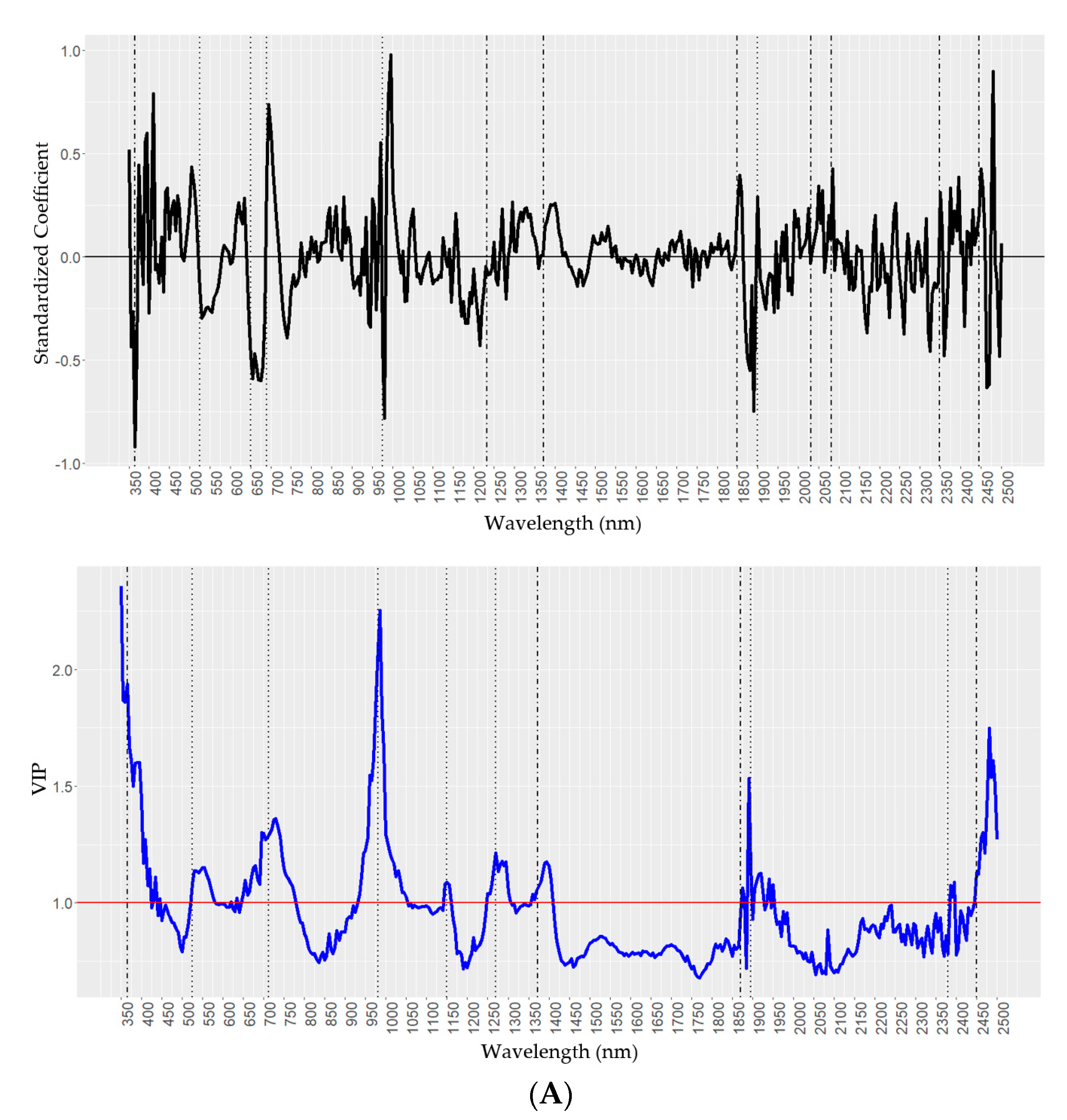
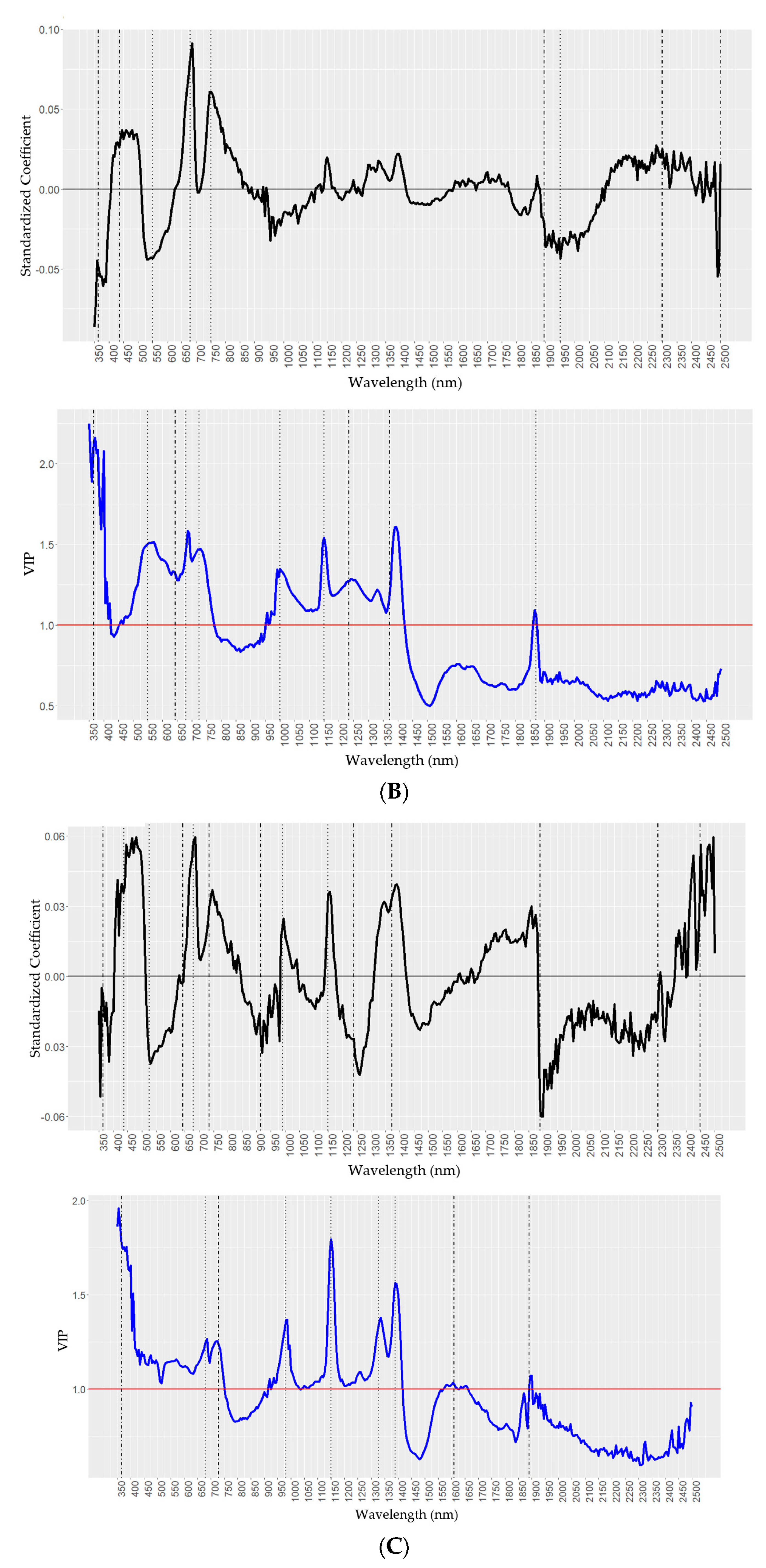
2.4. Predictions of Wax Components Using PLSR Models
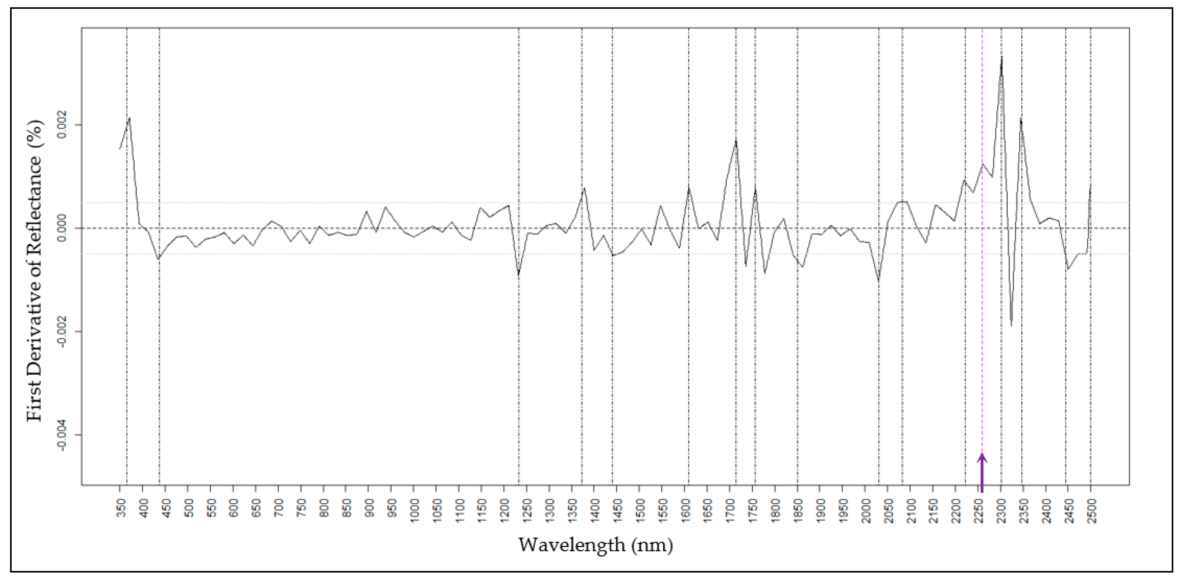
2.4.1. H16
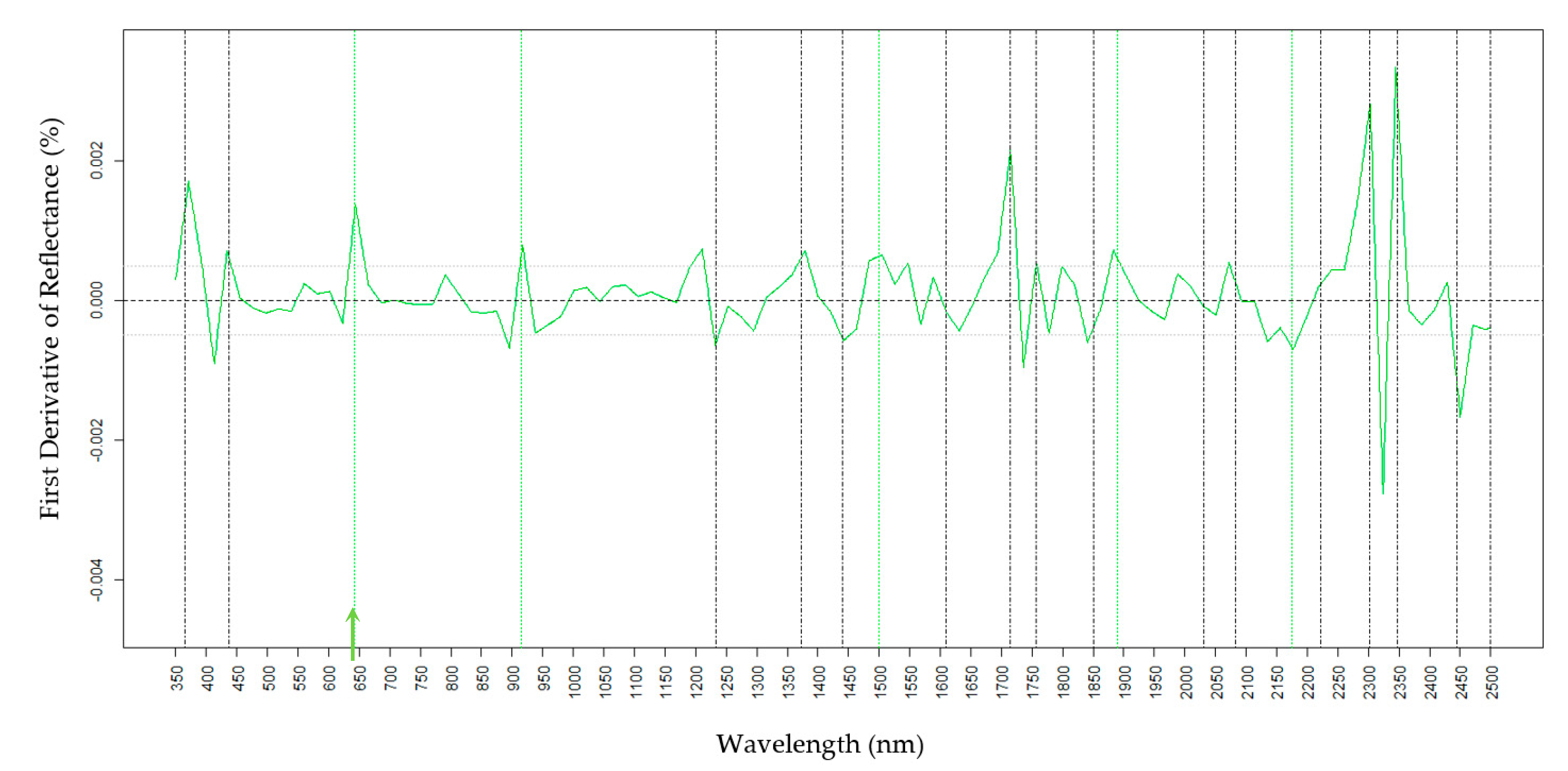
2.4.2. Oct
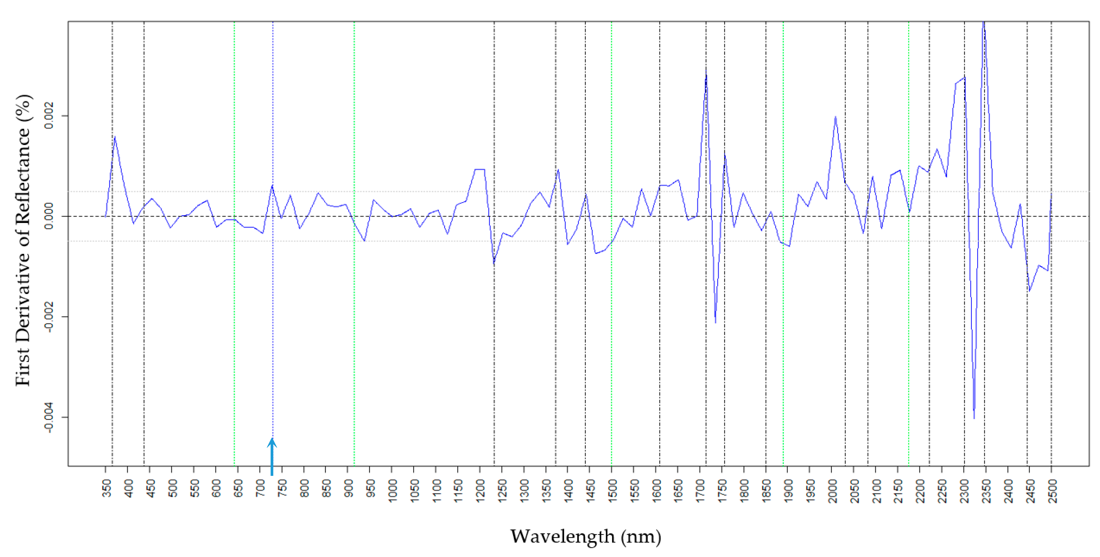
2.4.3. Tri
2.5. Genetic Mapping Using Spectrometric Measurements of H16, Oct, and Tri
3. Materials and Methods
3.1. Plant Materials
3.2. Spectral Measurements of Onion Leaves
3.3. Spectral Measurements of Chemical Standards
3.4. Gas Chromatography Gas Spectroscopy (GCMS)
3.5. Model Development
3.6. Data Analysis
3.7. QTL Analysis
4. Conclusions
Supplementary Materials
Author Contributions
Funding
Conflicts of Interest
Disclaimer
References
- Kokaly, R.F.; Asner, G.P.; Ollinger, S.V.; Martin, M.E.; Wessman, C.A. Characterizing canopy biochemistry from imaging spectroscopy and itsapplication to ecosystem studies. Remote Sens. Environ. 2009, 113, S78–S91. [Google Scholar] [CrossRef]
- Milton, E.J.; Schaepman, M.E.; Anderson, K.; Kneubühler, M.; Fox, N. Progress in field spectroscopy. Remote Sens. Environ. 2009, 113, S92–S109. [Google Scholar] [CrossRef]
- Schlemmer, M.; Gitelson, A.; Schepers, J.; Ferguson, R.; Peng, Y.; Shanahan, J.; Rundquist, D. Remote estimation of nitrogen and chlorophyll contents in maize at leaf and canopy levels. Int. J. Appl. Earth Obs. 2013, 25, 47–54. [Google Scholar] [CrossRef]
- Curran, P.J. Remote sensing of foliar chemistry. Remote Sens. Environ. 1989, 30, 271–278. [Google Scholar] [CrossRef]
- Hunt, E.R.; Doraiswamy, P.C.; McMurtrey, J.E.; Daughtry, C.S.T.; Perry, E.M.; Akhmedov, B. A visible band index for remote sensing leaf chlorophyll content at the canopy scale. Int. J. Appl. Earth Obs. 2013, 21, 103–112. [Google Scholar] [CrossRef]
- Malenovsk, Z.; Homolova, L.; Zurita-Milla, R.; Lukes, P.; Kaplan, V.; Hanus, J.; Gastellu-Etchegorry, J.P.; Schaepman, M.E. Retrieval of spruce leaf chlorophyll content from airborne image data using continuum removal and radiative transfer. Remote Sens. Environ. 2013, 131, 85–102. [Google Scholar] [CrossRef]
- Gitelson, A.; Keydan, G.P.; Merzlyak, M.N. Three-band model for noninvasive estimation of chlorophyll, carotenoids, and anthocyanin contents in higher plant leaves. Hydrol. Land Surf. Stud. 2006, 33, L11402. [Google Scholar] [CrossRef]
- Gitelson, A.A.; Zur, Y.; Chivkunova, O.B.; Merzlyak, M.N. Assessing carotenoid content in plant leaves with reflectance spectroscopy. Photochem. Photobiol. 2002, 75, 272–281. [Google Scholar] [CrossRef]
- Yuan, M.; Couture, J.J.; Townsend, P.A.; Ruark, M.D.; Bland, W.L. Spectroscopic determination of leaf nitrogen concentration and mass per area in sweet corn and snap bean. Agron. J. 2016, 108, 2519–2526. [Google Scholar] [CrossRef]
- Ainsworth, E.A.; Serbin, S.P.; Skoneczka, J.A.; Townsend, P.A. Using leaf optical properties to detect ozone effects on foliar biochemistry. Photosynth. Res. 2014, 119, 65–76. [Google Scholar] [CrossRef]
- Clevers, J.G.; Kooistra, L. Using hyperspectral remote sensing data for retrieving canopy chlorophyll and nitrogen content. IEEE J. STARS 2011, 5, 574–583. [Google Scholar] [CrossRef]
- Serbin, S.P.; Dillaway, D.N.; Kruger, E.L.; Townsend, P.A. Leaf optical properties reflect variation in photosynthetic metabolism and its sensitivity to temperature. J. Exp. Bot. 2012, 63, 489–502. [Google Scholar] [CrossRef]
- Vermerris, W.; Nicholson, R. The role of phenols in plant defense. In Phenolic Compound Biochemistry; Springer: Dordrecht, The Netherlands, 2008. [Google Scholar]
- Couture, J.J.; Serbin, S.P.; Townsend, P.A. Spectroscopic sensitivity of real-time, rapidly induced phytochemical change in response to damage. New Phytol. 2013, 198, 311–319. [Google Scholar] [CrossRef] [PubMed]
- Kokalya, R.F.; Skidmore, A.K. Plant phenolics and absorption features in vegetation reflectance spectra near 1.66 μm. Int. J. Appl. Earth Obs. 2015, 43, 55–83. [Google Scholar] [CrossRef]
- Leucker, M.; Mahlein, A.K.; Steiner, U.; Oerke, E.C. Improvement of lesion phenotyping in Cercospora beticola-sugar beet interaction by hyperspectral imaging. Phytopathology 2016, 106, 177–184. [Google Scholar] [CrossRef] [PubMed]
- Bálint, J.; Nagy, B.V.; Fail, J.; Ghanim, M. Correlations between colonization of onion thrips and leaf reflectance measures across six cabbage varieties. PLoS ONE 2013, 8, e73848. [Google Scholar] [CrossRef]
- Fletcher, R.S.; Smith, J.R.; Mengistu, A.; Ray, J.D. Relationships between Microsclerotia Content and Hyperspectral Reflectance Data in Soybean Tissue Infected by Macrophomina phaseolina. Am. J. Plant Sci. 2014, 5, 3737–3744. [Google Scholar] [CrossRef]
- Kuska, M.; Wahabzada, M.; Leucker, M.; Dehne, H.-W.; Kersting, K.; Oerke, E.-C.; Steiner, U.; Mahlein, A.-K. Hyperspectral phenotyping on the microscopic scale: Towards automated characterization of plant-pathogen interactions. Plant Methods 2015, 11, 28. [Google Scholar] [CrossRef]
- Ribeiro da Luz, B. Attenuated total reflectance spectroscopy of plant leaves: A tool for ecological and botanical studies. New Phytol. 2006, 172, 305–318. [Google Scholar] [CrossRef]
- Jenks, M.A.; Tuttle, H.A.; Eigenbrode, S.D.; Feldmann, K.A. Leaf epicuticular waxes of the eceriferum mutants in Arabidopsis. Plant Physiol. 1995, 108, 369–377. [Google Scholar] [CrossRef]
- Bernard, A.; Joubès, J. Arabidopsis cuticular waxes: Advances in synthesis, export and regulation. Prog. Lipid. Res. 2013, 52, 110–129. [Google Scholar] [CrossRef] [PubMed]
- Lee, S.B.; Suh, M.C. Recent advances in cuticular wax biosynthesis and its regulation in Arabidopsis. Mol. Plant 2013, 6, 246–249. [Google Scholar] [CrossRef] [PubMed]
- Rhee, Y.; Hlousek-Radojcic, A.; Ponsamuel, P.; Liu, D.; Beittenmiller, P. Epicuticular wax accumulation and fatty acid elongation activities are induced during leaf development of leeks. Plant Physiol. 1998, 116, 901–911. [Google Scholar] [CrossRef] [PubMed]
- Damon, S.J.; Groves, R.L.; Havey, M.J. Variation for epicuticular waxes on onion foliage and impacts on numbers of onion thrips. J. Am. Soc. Hortic. Sci. 2014, 139, 495–501. [Google Scholar] [CrossRef]
- Munaiz, E.D.; Groves, R.L.; Havey, M.J. Amounts and Types of Epicuticular Leaf Waxes among Onion Accessions Selected for Reduced Damage by Onion Thrips. J. Am. Soc. Hortic. Sci. 2019, 1, 1–6. [Google Scholar] [CrossRef]
- Jones, H.A.; Bailey, S.F.; Emsweller, S.L. Thrips resistance in onion. Hilgardia 1934, 8, 215–232. [Google Scholar] [CrossRef]
- Eigenbrode, S.D.; Espelie, K.E. Effects of plant epicuticular lipids on insect herbivores. Annu. Rev. Entomol. 1995, 40, 171–194. [Google Scholar] [CrossRef]
- Pawar, B.B.; Patil, A.V.; Sonone, H.N. A thrips resistant glossy selection in white onions. Res. J. Mahatma Phule Agric. Univ. 1975, 6, 152–153. [Google Scholar]
- Alimousavi, S.A.; Hassandokht, M.R.; Moharramipour, S. Evaluation of Iranian onion germplasms for resistance to thrips. Int. J. Agric. Biol. 2007, 9, 897–900. [Google Scholar]
- Diaz-Montano, J.; Fuchs, M.; Nault, B.A.; Shelton, A.M. Evaluation of onion cultivars for resistance to onion Thrips (Thysanoptera: Thripidae) and Iris Yellow Spot Virus. J. Econ. Entomol. 2010, 103, 925–937. [Google Scholar] [CrossRef]
- Woolbright, S.A. Large effect quantitative trait loci for salicinoid phenolic glycosides in Populus: Implications for gene discovery. Ecol. Evol. 2018, 8, 3726–3737. [Google Scholar] [CrossRef]
- Couture, J.J.; Singh, A.; Rubert-Nason, K.F.; Serbin, S.P.; Lindroth, R.L.; Townsend, P.A. Spectroscopic determination of ecologically relevant plant secondary metabolites. Methods Ecol. Evol. 2016, 7, 1402–1412. [Google Scholar] [CrossRef]
- Munaiz, E.D.; Havey, M.J. Genetic Analyses of Epicuticular Waxes Associated with the Glossy Foliage of ‘White Persian’Onion. J. Am. Soc. Hortic. Sci. 2020, 145, 67–72. [Google Scholar] [CrossRef]
- Hyde, P.T.; Earle, E.D.; Mutschler, M.A. Doubled haploid onion (Allium cepa L.) lines and their impact on hybrid performance. HortScience 2012, 47, 1690–1695. [Google Scholar] [CrossRef]
- Gülz, P.G.; Müller, E.; Schmitz, K. Chemical composition and surface structures of epicuticular leaf waxes of Ginkgo biloba, Magnolia grandiflora and Liriodendron tulipifera. Z. Nat. 1992, 47, 516–526. [Google Scholar] [CrossRef]
- Singh, A.; Serbin, S.P.; McNeil, B.E.; Kingdon, C.C.; Townsend, P.A. Imaging spectroscopy algorithms for mapping canopy foliar chemical and morphological traits and their uncertainties. Ecol. Appl. 2015, 25, 2180–2197. [Google Scholar] [CrossRef]
- Zhai, Y.; Cui, L.; Zhou, X.; Gao, Y.; Fei, T.; Gao, W. Estimation of nitrogen, phosphorus, and potassium contents in the leaves of different plants using laboratory-based visible and near-infrared reflectance spectroscopy: Comparison of partial least-square regression and support vector machine regression methods. Int. J. Remote Sens. 2013, 34, 2502–2518. [Google Scholar]
- Elvidge, C.D. Visible and near infrared reflectance characteristics of dry plant materials. Remote Sens. 1990, 11, 1775–1795. [Google Scholar] [CrossRef]
- Yang, L.; Liu, Q.; Wang, Y.; Liu, L. Identification and characterization of a glossy mutant in Welsh onion (Allium fistulosum L.). Sci. Hortic. 2017, 225, 122–127. [Google Scholar] [CrossRef]
- Hoagland, D.; Snyder, W. Nutrition of strawberry plant under controlled conditions: (a) effects of deficiencies of boron and certain other elements: (b) susceptibility to injury from sodium salts. Proc. Am Soc. Hortic. Sci 1933, 30, 288–941. [Google Scholar]
- Wold, S.; Ruhe, A.; Wold, H.; Dunn, W.J. The collinearity problem in linear regression. The Partial Least Squares (PLS) approach to generalized inverses. SIAM J. Sci. Stat. Comput. 1984, 5, 735–743. [Google Scholar] [CrossRef]
- Wold, S.; Sjöström, M.; Eriksson, L. PLS-Regression: A basic tool of chemometrics. Chemom. Intell. Lab. Syst. 2001, 58, 109–130. [Google Scholar] [CrossRef]
- Gelad, P.; Kowalski, B.R. Partial Least-Squares Regression: A Tutorial; Elsevier Science Publishers B.V.: Amsterdam, The Netherlands, 1986; Volume 185. [Google Scholar]
- Serbin, S.P.; Singh, A.; McNeil, B.E.; Kingdon, C.C.; Townsend, P.A. Spectroscopic determination of leaf morphological and biochemical traits for northern temperate and boreal tree species. Ecol. Appl. 2014, 24, 1651–1669. [Google Scholar] [CrossRef] [PubMed]
- Chen, S.; Hong, X.; Harris, C.J.; Sharkey, P.M. Spare modeling using orthogonal forest regression with PRESS statistic and regularization. IEEE Trans. Syst. Man Cybern. 2004, 34, 898–911. [Google Scholar] [CrossRef] [PubMed]
- R Core Team. R: A Language and Environment for Statistical Computing; R Foundation for Statistical Computing: Vienna, Austria, 2014. [Google Scholar]
- Wold, S. PLS for multivariate linear modeling. In Chemometricmethods in Molecular Design, Methods and Principles Inmedicinal Chemistry; Van de Waterbeemd, H., Ed.; Verlag-Chemie: Weinheim, Germany, 1994; pp. 195–218. [Google Scholar]
- Broman, K.W.; Wu, H.; Sen, S.; Churchill, G.A. R/qtl: QTL mapping in experimental crosses. Comput. Appl. Biosci. 2003, 19, 889–890. [Google Scholar] [CrossRef] [PubMed]
- Haley, C.S.; Knott, S.A. A simple regression method for mapping quantitative trait loci in line crosses using flanking markers. Heredity 1992, 69, 315–324. [Google Scholar] [CrossRef]
Sample Availability: Plant materials are available from the corresponding author. |


| Accession z | ‘Cultivar’ and Origin | Phenotype y |
|---|---|---|
| B9885 | ‘White Persian’, Iran | GL |
| 289689 | ‘Odourless Green Leaf’, Australia | GL |
| 546115 | ‘White Sweet Spanish Jumbo’, USA | SG |
| 546192 | ‘Yellow Sweet Spanish’, USA | SG |
| 264320 | ‘Grano’, Spain | SG |
| B5351 | ‘Sweet Spanish Colorado #6′, USDA | SG |
| DH2107 | Cornell University, USA | WX |
| Accession z | Phenotype x | H16 | SE | Oct | SE | Tri | SE | |||
|---|---|---|---|---|---|---|---|---|---|---|
| OGL | GL | 0.002 y | 0.088 | a | 0.554 | 0.037 | c | 0.000 | 0.025 | a |
| 546115 | SG | 0.532 | 0.088 | b | 0.364 | 0.037 | b | 0.223 | 0.025 | cd |
| 546192 | SG | 0.642 | 0.124 | bc | 0.454 | 0.037 | bc | 0.195 | 0.025 | bcd |
| B5351 | SG | 0.648 | 0.088 | b | 0.141 | 0.053 | a | 0.075 | 0.036 | ab |
| B9885 | GL | 0.700 | 0.088 | bc | 0.444 | 0.037 | bc | 0.140 | 0.025 | bc |
| 264320 | SG | 1.091 | 0.088 | c | 0.586 | 0.037 | c | 0.247 | 0.025 | cd |
| DH2107 | WX | 2.015 | 0.088 | d | 0.496 | 0.037 | bc | 0.260 | 0.025 | d |
| Accession z | Phenotype y | Waxes | |||||||
|---|---|---|---|---|---|---|---|---|---|
| H16 | Oct | Tri | Met | Hex | Octd | Hepc | Hepd | ||
| OGL | GL | 0.3 | 70.7 | 0.0 | 0.1 | 19.2 | 9.6 | 0.0 | 0.0 |
| 546115 | SG | 36.8 | 25.1 | 15.4 | 2.8 | 11.1 | 0.2 | 4.8 | 3.7 |
| 546192 | SG | 40.6 | 28.7 | 12.3 | 3.8 | 3.2 | 1.2 | 6.0 | 4.1 |
| B5351 | SG | 52.9 | 11.5 | 6.1 | 5.0 | 1.1 | 2.5 | 12.0 | 8.9 |
| B9885 | GL | 44.4 | 28.2 | 8.9 | 2.5 | 3.8 | 3.9 | 3.1 | 5.2 |
| 264320 | SG | 48.1 | 25.8 | 10.9 | 2.7 | 4.5 | 1.1 | 3.4 | 3.4 |
| DH2107 | WX | 65.0 | 16.0 | 8.4 | 1.5 | 2.4 | 0.9 | 2.2 | 3.6 |
| Wax | Cross Validation | Validation y | ||||||
|---|---|---|---|---|---|---|---|---|
| R2 | RMSE | % | Range | R2 | RMSE | % | Range | |
| H16 | 0.86 | 0.182 | 8.25 | 0–2.20 | 0.72 | 0.304 | 12.62 | 0–2.41 |
| Oct | 0.67 | 0.108 | 14.03 | 0–0.77 | 0.70 | 0.102 | 15.47 | 0–0.66 |
| Tri | 0.48 | 0.068 | 16.38 | 0–0.41 | 0.41 | 0.072 | 20.73 | 0–0.35 |
| Chemical y | Standardized Coefficients z | VIP z |
|---|---|---|
| H16 (nm) | 365, 525, 650, 690, 975, 1233, 1372, 1850, 1900, 2031, 2082, 2348, and 2445 | 365, 525, 712, 980, 1150,1270, 1372, 1860, 1895, 2380, and 2450 |
| Oct (nm) | 365, 437, 550, 680, 750, 1890, 1950, 2300, and 2499 | 365, 550, 645, 680, 725, 1000, 1150, 1233, 1372, and 1870 |
| Tri (nm) | 365, 437, 525, 643, 680, 730, 915, 991, 1150, 1233, 1372, 1890, 2302, and 2449 | 365, 680,730, 980, 1150, 1328, 1390, 1610, and 1890 |
| Trait | Chr | Pos | SNP z | 1.5 LOD Interval z | % Var | LOD | Thresh | Add y | Dom y |
|---|---|---|---|---|---|---|---|---|---|
| H16 (Spectroscopy) | 8 | 41.1 | i19082_1721 | i28432_1302-i28633_2705 | 21.0 | 4.9 | 2.9 | 0.10 | 0.14 |
| H16 (GCMS) | 8 | 41.1 | i19082_1721 | i41653_558-i20235_630 | 45.6 | 15.8 | 9.3 | 0.57 | 0.33 |
| Oct (Spectroscopy) | 8 | 41.1 | i19082_1721 | i29044_2564-i28633_2705 | 21.0 | 3.8 | 3.5 | 0.36 | 0.31 |
| Oct (GCMS) | 8 | 46.2 | i20235_630 | i19082_1721–i28633_2705 | 16.9 | 3.7 | 3.5 | 0.36 | 0.31 |
| Tri (Spectroscopy) | 8 | 41.1 | i19082_1721 | i41653_558-i20235_630 | 36.4 | 9.1 | 3.6 | 0.29 | 0.28 |
| Tri (GCMS) | 8 | 46.2 | i20235_630 | i19082_1721–i28633_2705 | 23.3 | 5.5 | 3.6 | 0.30 | 0.19 |
© 2020 by the authors. Licensee MDPI, Basel, Switzerland. This article is an open access article distributed under the terms and conditions of the Creative Commons Attribution (CC BY) license (http://creativecommons.org/licenses/by/4.0/).
Share and Cite
Munaiz, E.D.; Townsend, P.A.; Havey, M.J. Reflectance Spectroscopy for Non-Destructive Measurement and Genetic Analysis of Amounts and Types of Epicuticular Waxes on Onion Leaves. Molecules 2020, 25, 3454. https://doi.org/10.3390/molecules25153454
Munaiz ED, Townsend PA, Havey MJ. Reflectance Spectroscopy for Non-Destructive Measurement and Genetic Analysis of Amounts and Types of Epicuticular Waxes on Onion Leaves. Molecules. 2020; 25(15):3454. https://doi.org/10.3390/molecules25153454
Chicago/Turabian StyleMunaiz, Eduardo D., Philip A. Townsend, and Michael J. Havey. 2020. "Reflectance Spectroscopy for Non-Destructive Measurement and Genetic Analysis of Amounts and Types of Epicuticular Waxes on Onion Leaves" Molecules 25, no. 15: 3454. https://doi.org/10.3390/molecules25153454
APA StyleMunaiz, E. D., Townsend, P. A., & Havey, M. J. (2020). Reflectance Spectroscopy for Non-Destructive Measurement and Genetic Analysis of Amounts and Types of Epicuticular Waxes on Onion Leaves. Molecules, 25(15), 3454. https://doi.org/10.3390/molecules25153454