
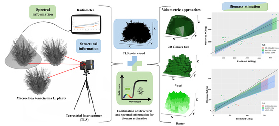
Non-Destructive Biomass Estimation in Mediterranean Alpha Steppes: Improving Traditional Methods for Measuring Dry and Green Fractions by Combining Proximal Remote Sensing Tools

 ,
,  ,
, 
Abstract
1. Introduction
2. Methods
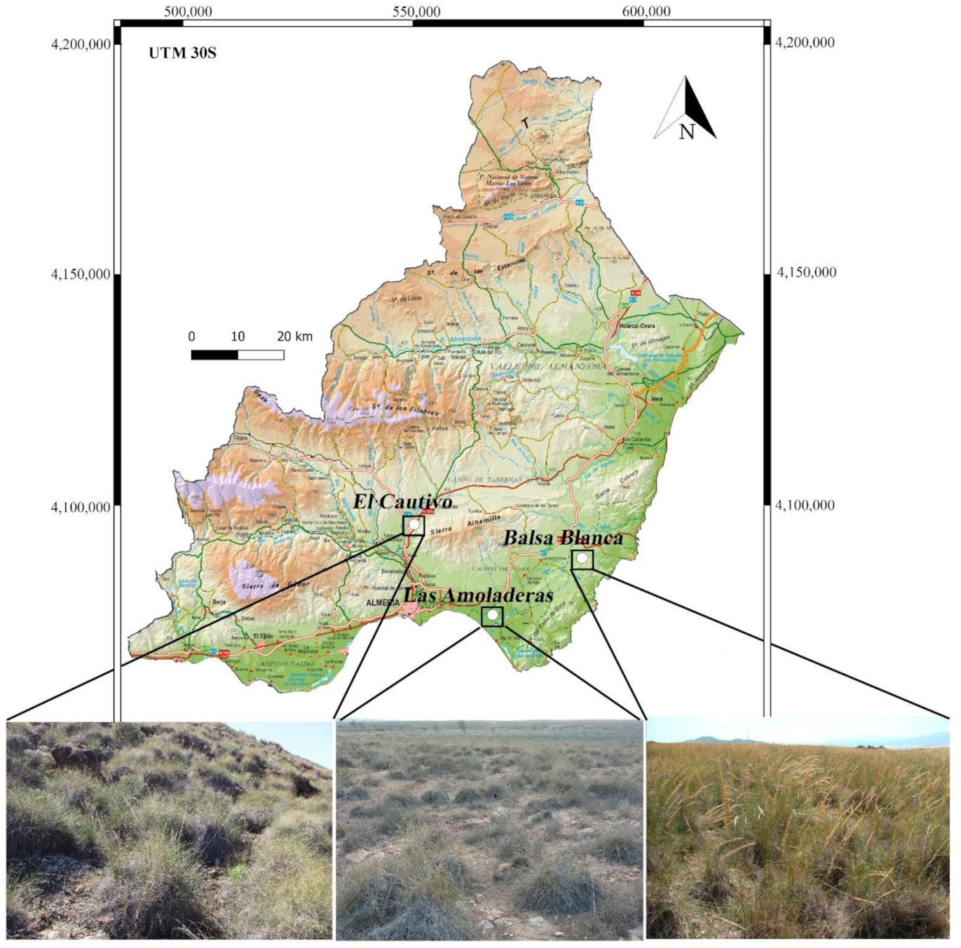
2.1. Study Sites and Field Sampling
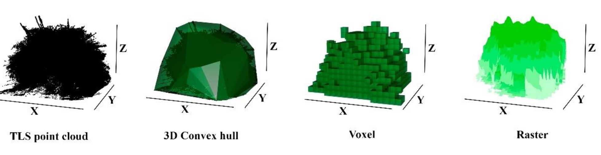
2.2. TLS Data Processing and Volume Estimation
2.3. Field Spectra Data Pre-Processing
2.4. Plant Biomass Estimation
2.5. Green Biomass Estimation
3. Results
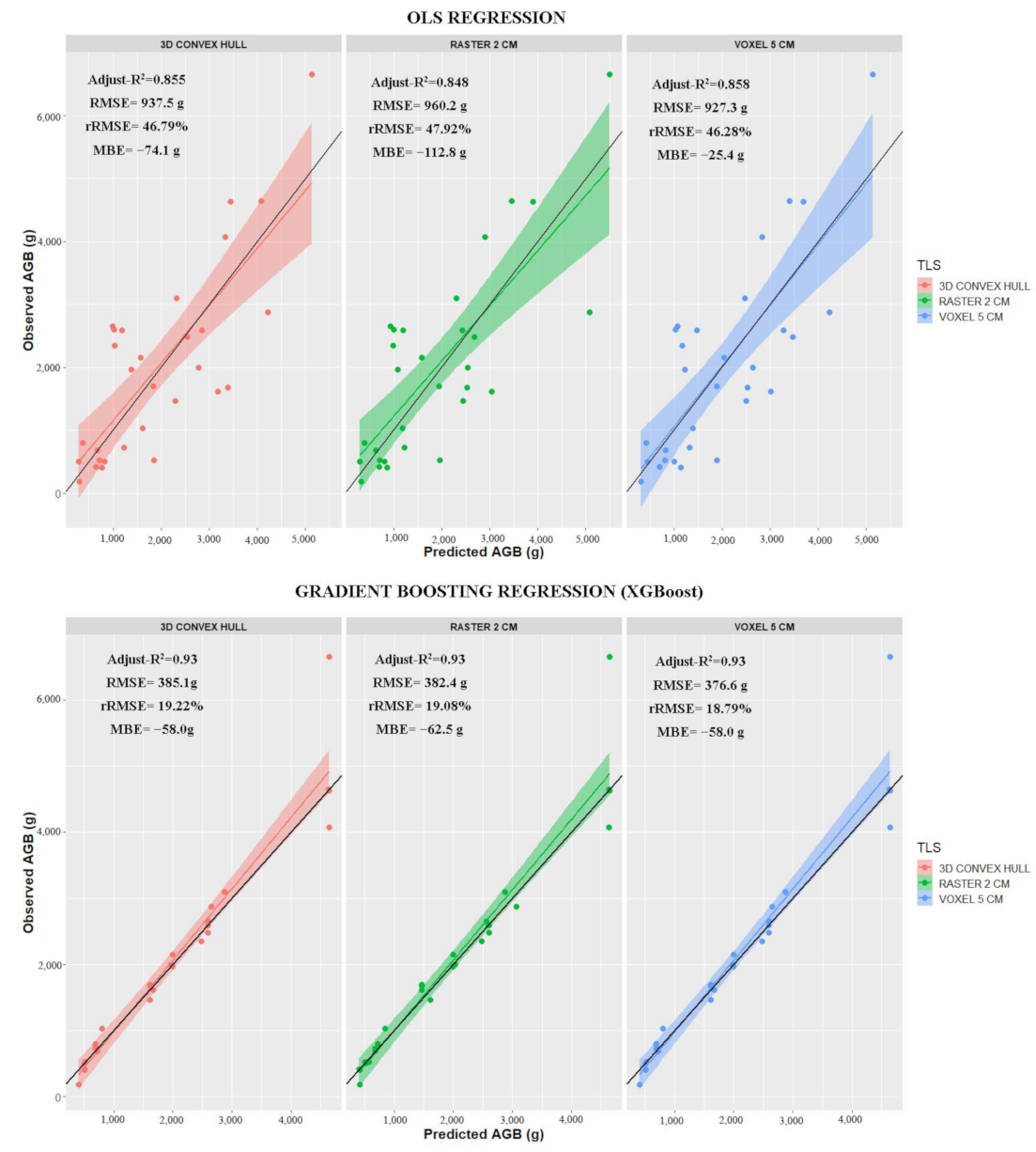
3.1. Total Biomass Estimation
3.2. Photosynthetic Biomass Estimation
4. Discussion
5. Conclusions
Supplementary Materials
Author Contributions
Funding
Institutional Review Board Statement
Informed Consent Statement
Data Availability Statement
Acknowledgments
Conflicts of Interest
References
- Vashum, K.; Jayakumar, S. Methods to Estimate Above-Ground Biomass and Carbon Stock in Natural Forests—A Review. J. Ecosyst. Ecogr. 2012, 2. [Google Scholar] [CrossRef]
- Borah, N.; Jyoti, A.; Kumar, A. Aboveground biomass and carbon stocks of tree species in tropical forests of Cachar District, Assam, Northest India. Int. J. Ecol. Environ. Sci. 2013, 39, 97–106. [Google Scholar]
- Yalçin, E. The relationships among aboveground biomass, primary productivity, precipitation and temperature in grazed aun ungrazed temperate grassland from northern turkey. Black Sea J. Eng. Sci. 2018, 1, 107–113. [Google Scholar]
- Gyssels, G.; Poesen, J.; Bochet, E.; Li, Y. Impact of plant roots on the resistance of soils to erosion by water: A review. Prog. Phys. Geogr. 2005, 29, 189–217. [Google Scholar] [CrossRef]
- Li, S.; Su, J.; Lang, X.; Liu, W.; Ou, G.; Xu, H.; Su, J. Positive relationship between species richness and aboveground biomass across forest strata in a primary Pinus kesiya forest. Sci. Rep. 2018, 8, 2227. [Google Scholar] [CrossRef] [PubMed]
- Vargas, L.; Willemen, L.; Hein, L. Assessing the Capacity of Ecosystems to Supply Ecosystem Services Using Remote Sensing and an Ecosystem Accounting Approach. Environ. Manag. 2019, 63, 1–15. [Google Scholar] [CrossRef] [PubMed]
- Chave, J.; Olivier, J.; Bongers, F.; Châtelet, P.; Forget, P.M.; Van Der Meer, P.; Norden, N.; Riéra, B.; Charles-Dominique, P. Above-ground biomass and productivity in a rain forest of eastern South America. J. Trop. Ecol. 2008, 24, 355–366. [Google Scholar] [CrossRef]
- Zhao, F.; Xu, B.; Yang, X.; Jin, Y.; Li, J.; Xia, L.; Chen, S.; Ma, H. Remote sensing estimates of grassland aboveground biomass based on MODIS Net Primary Productivity (NPP): A case study in the Xilingol grassland of northern China. Remote Sens. 2014, 6, 5368–5386. [Google Scholar] [CrossRef]
- Wang, Y.; Meng, B.; Zhong, S.; Wang, D.; Ma, J.; Sun, W. Aboveground biomass and root/shoot ratio regulated drought susceptibility of ecosystem carbon exchange in a meadow steppe. Plant Soil 2018, 432, 259–272. [Google Scholar] [CrossRef]
- Conti, G.; Enrico, L.; Casanoves, F.; Díaz, S. Shrub biomass estimation in the semiarid Chaco forest: A contribution to the quantification of an underrated carbon stock. Ann. For. Sci. 2013, 70, 515–524. [Google Scholar] [CrossRef]
- Becknell, J.M.; Powers, J.S. Stand age and soils as drivers of plant functional traits and aboveground biomass in secondary tropical dry forest. Can. J. For. Res. 2014, 44, 604–613. [Google Scholar] [CrossRef]
- Bonham, C.D. Measurements for Terrestrial Vegetation, 1st ed.; Wiley-Interscience, Ed.; Wiley: New York, NY, USA, 1989; ISBN 9780471048800. [Google Scholar]
- Jonasson, S. Evaluation of the Point Intercept Method for the Estimation of Plant Evaluation of the point intercept method for the estimation of plant biomass. Oikos 1988, 52, 101–106. [Google Scholar] [CrossRef]
- Clark, P.E.; Hardegree, S.P.; Moffet, C.A.; Pierson, F.B. Point sampling to stratify biomass variability in sagebrush steppe vegetation. Rangel. Ecol. Manag. 2008, 61, 614–622. [Google Scholar] [CrossRef]
- Yuen, J.Q.; Fung, T.; Ziegler, A.D. Review of allometric equations for major land covers in SE Asia: Uncertainty and implications for above- and below-ground carbon estimates. For. Ecol. Manag. 2016, 360, 323–340. [Google Scholar] [CrossRef]
- Moundounga Mavouroulou, Q.; Ngomanda, A.; Engone Obiang, N.L.; Lebamba, J.; Gomat, H.; Mankou, G.S.; Loumeto, J.; Midoko Iponga, D.; Kossi Ditsouga, F.; Zinga Koumba, R.; et al. How to improve allometric equations to estimate forest biomass stocks? Some hints from a central African forest. Can. J. For. Res. 2014, 44, 685–691. [Google Scholar] [CrossRef]
- Xie, Y.; Sha, Z.; Yu, M. Remote sensing imagery in vegetation mapping: A review. J. Plant Ecol. 2008, 1, 9–23. [Google Scholar] [CrossRef]
- Xue, J.; Su, B. Significant remote sensing vegetation indices: A review of developments and applications. J. Sens. 2017, 2017. [Google Scholar] [CrossRef]
- Zhang, X.; Friedl, M.A.; Schaaf, C.B.; Strahler, A.H.; Hodges, J.C.F.; Gao, F.; Reed, B.C.; Huete, A. Monitoring vegetation phenology using MODIS. Remote Sens. Environ. 2003, 84, 471–475. [Google Scholar] [CrossRef]
- Liu, S.; Su, X.; Dong, S.; Cheng, F.; Zhao, H.; Wu, X.; Zhang, X.; Li, J. Modeling aboveground biomass of an alpine desert grassland with SPOT-VGT NDVI. GIScience Remote Sens. 2015, 52, 680–699. [Google Scholar] [CrossRef]
- Hilker, T.; Wulder, M.A.; Coops, N.C.; Linke, J.; McDermid, G.; Masek, J.G.; Gao, F.; White, J.C. A new data fusion model for high spatial- and temporal-resolution mapping of forest disturbance based on Landsat and MODIS. Remote Sens. Environ. 2009, 113, 1613–1627. [Google Scholar] [CrossRef]
- Zúñiga-Vásquez, J.M.; Aguirre-Salado, C.A.; Pompa-García, M. Monitoring vegetation using remote sensing time series data: A review of the period 1996–2017. Rev. Fac. Cienc. Agrar. 2020, 52, 175–189. [Google Scholar]
- Asner, G.P.; Martin, R.E. Spectranomics: Emerging science and conservation opportunities at the interface of biodiversity and remote sensing. Glob. Ecol. Conserv. 2016, 8, 212–219. [Google Scholar] [CrossRef]
- Friedel, M.H.; Laycock, W.A.; Bastin, G.N. Assessing rangeland condition and trend. In Field and Laboratory Methods for Grassland and Animal Production Research; ’t Mannetje, L., Jones, R.M., Eds.; CABI Publihing: Wageningen, The Netherlands, 2000; ISBN 9780851993515. [Google Scholar]
- Huang, W.; Lamb, D.W.; Niu, Z.; Zhang, Y.; Liu, L.; Wang, J. Identification of yellow rust in wheat using in-situ spectral reflectance measurements and airborne hyperspectral imaging. Precis. Agric. 2007, 8, 187–197. [Google Scholar] [CrossRef]
- Brinkmann, K.; Dickhoefer, U.; Schlecht, E.; Buerkert, A. Quantification of aboveground rangeland productivity and anthropogenic degradation on the Arabian Peninsula using Landsat imagery and field inventory data. Remote Sens. Environ. 2011, 115, 465–474. [Google Scholar] [CrossRef]
- Benseghir, L.; Kadi-Hanifi, H.; Bachari, N.E.I. Estimation of aboveground biomass in conserved areas of Stipa tenacissima L. stands in the high steppes of western Algeria by mean of the Landsat 8 imagery-based vegetation indices. Afr. J. Ecol. 2019, 57, 466–476. [Google Scholar] [CrossRef]
- Nguyen, T.H.; Jones, S.; Soto-Berelov, M.; Haywood, A.; Hislop, S. Landsat time-series for estimating forest aboveground biomass and its dynamics across space and time: A review. Remote Sens. 2020, 12, 98. [Google Scholar] [CrossRef]
- Rodríguez-Caballero, E.; Knerr, T.; Weber, B. Importance of biocrusts in dryland monitoring using spectral indices. Remote Sens. Environ. 2015, 170, 32–39. [Google Scholar] [CrossRef]
- Smith, W.K.; Dannenberg, M.P.; Yan, D.; Herrmann, S.; Barnes, M.L.; Barron-Gafford, G.A.; Biederman, J.A.; Ferrenberg, S.; Fox, A.M.; Hudson, A.; et al. Remote sensing of dryland ecosystem structure and function: Progress, challenges, and opportunities. Remote Sens. Environ. 2019, 233, 111401. [Google Scholar] [CrossRef]
- Lefsky, M.A.; Cohen, W.B.; Harding, D.J.; Parker, G.G.; Acker, S.A.; Gower, S.T. Lidar remote sensing of above-ground biomass in three biomes. Glob. Ecol. Biogeogr. 2002, 11, 393–399. [Google Scholar] [CrossRef]
- Zolkos, S.G.; Goetz, S.J.; Dubayah, R. A meta-analysis of terrestrial aboveground biomass estimation using lidar remote sensing. Remote Sens. Environ. 2013, 128, 289–298. [Google Scholar] [CrossRef]
- Fallah, Y.; Onur, M. Lidar for Biomass Estimation. In Biomass—Detection, Production and Usage; Matovic, D., Ed.; IntechOpen: London, UK, 2011; pp. 1–21. [Google Scholar] [CrossRef]
- Stovall, A.E.L.; Shugart, H.H.; Stovall, A.E.L.; Anderson-Teixeira, K.J.; Anderson-Teixeira, K.J. Assessing terrestrial laser scanning for developing non-destructive biomass allometry. For. Ecol. Manag. 2018, 427, 217–229. [Google Scholar] [CrossRef]
- Olsoy, P.J.; Glenn, N.F.; Clark, P.E.; Derryberry, D.W.R. Aboveground total and green biomass of dryland shrub derived from terrestrial laser scanning. ISPRS J. Photogramm. Remote Sens. 2014, 88, 166–173. [Google Scholar] [CrossRef]
- Stovall, A.E.L.; Vorster, A.G.; Anderson, R.S.; Evangelista, P.H.; Shugart, H.H. Non-destructive aboveground biomass estimation of coniferous trees using terrestrial LiDAR. Remote Sens. Environ. 2017, 200, 31–42. [Google Scholar] [CrossRef]
- Seidel, D.; Fleck, S.; Leuschner, C.; Hammett, T. Review of ground-based methods to measure the distribution of biomass in forest canopies. Ann. For. Sci. 2011, 68, 225–244. [Google Scholar] [CrossRef]
- Olsoy, P.J.; Glenn, N.F.; Clark, P.E. Estimating sagebrush biomass using terrestrial laser scanning. Rangel. Ecol. Manag. 2014, 67, 224–228. [Google Scholar] [CrossRef]
- Olsoy, P.J.; Mitchell, J.J.; Levia, D.F.; Clark, P.E.; Glenn, N.F. Estimation of big sagebrush leaf area index with terrestrial laser scanning. Ecol. Indic. 2016, 61, 815–821. [Google Scholar] [CrossRef]
- Nölke, N.; Fehrmann, L.; Jaya, I.N.S.; Tiryana, T.; Seidel, D.; Kleinn, C. On the geometry and allometry of big-buttressed trees—A challenge for forest monitoring: New insights from 3D-modeling with terrestrial laser scanning. IForest 2015, 8, 574–581. [Google Scholar] [CrossRef]
- Li, A.; Glenn, N.F.; Olsoy, P.J.; Mitchell, J.J.; Shrestha, R. Aboveground biomass estimates of sagebrush using terrestrial and airborne LiDAR data in a dryland ecosystem. Agric. For. Meteorol. 2015, 213, 138–147. [Google Scholar] [CrossRef]
- Brede, B.; Calders, K.; Lau, A.; Raumonen, P.; Bartholomeus, H.M.; Herold, M.; Kooistra, L. Non-destructive tree volume estimation through quantitative structure modelling: Comparing UAV laser scanning with terrestrial LIDAR. Remote Sens. Environ. 2019, 233, 111355. [Google Scholar] [CrossRef]
- Rahman, M.Z.A.; Bakar, M.A.A.; Razak, K.A.; Rasib, A.W.; Kanniah, K.D.; Kadir, W.H.W.; Omar, H.; Faidi, A.; Kassim, A.R.; Latif, Z.A. Non-destructive, laser-based individual tree aboveground biomass estimation in a tropical rainforest. Forests 2017, 8, 86. [Google Scholar] [CrossRef]
- Wallace, L.; Hillman, S.; Reinke, K.; Hally, B. Non-destructive estimation of above-ground surface and near-surface biomass using 3D terrestrial remote sensing techniques. Methods Ecol. Evol. 2017, 8, 1607–1616. [Google Scholar] [CrossRef]
- Greaves, H.E.; Vierling, L.A.; Eitel, J.U.H.; Boelman, N.T.; Magney, T.S.; Prager, C.M.; Griffin, K.L. Estimating aboveground biomass and leaf area of low-stature Arctic shrubs with terrestrial LiDAR. Remote Sens. Environ. 2015, 164, 26–35. [Google Scholar] [CrossRef]
- Hopkinson, C.; Chasmer, L.; Colville, D.; Fournier, R.A.; Hall, R.J.; Luther, J.E.; Milne, T.; Petrone, R.M.; St-Onge, B. Moving toward consistent ALS monitoring of forest attributes across Canada: A consortium approach. Photogramm. Eng. Remote Sens. 2013, 79, 159–173. [Google Scholar] [CrossRef]
- Casas, A.; Riaño, D.; Ustin, S.L.; Dennison, P.; Salas, J. Estimation of water-related biochemical and biophysical vegetation properties using multitemporal airborne hyperspectral data and its comparison to MODIS spectral response. Remote Sens. Environ. 2014, 148, 28–41. [Google Scholar] [CrossRef]
- Varga, T.A.; Asner, G.P. Hyperspectral and LiDAR remote sensing of fire fuels in Hawaii volcanoes National Park. Ecol. Appl. 2008, 18, 613–623. [Google Scholar] [CrossRef] [PubMed]
- Jacquemoud, S.; Verhoef, W.; Baret, F.; Bacour, C.; Zarco-Tejada, P.J.; Asner, G.P.; François, C.; Ustin, S.L. PROSPECT + SAIL models: A review of use for vegetation characterization. Remote Sens. Environ. 2009, 113, S56–S66. [Google Scholar] [CrossRef]
- Estornell, J.; Ruiz, L.A.; Velázquez-Martí, B.; Fernández-Sarría, A. Estimation of shrub biomass by airborne LiDAR data in small forest stands. For. Ecol. Manag. 2011, 262, 1697–1703. [Google Scholar] [CrossRef]
- Estornell, J.; Ruiz, L.A.; Velázquez-Martí, B.; Hermosilla, T. Estimation of biomass and volume of shrub vegetation using LiDAR and spectral data in a Mediterranean environment. Biomass Bioenergy 2012, 46, 710–721. [Google Scholar] [CrossRef]
- Huang, C.Y.; Anderegg, W.R.L.; Asner, G.P. Remote sensing of forest die-off in the Anthropocene: From plant ecophysiology to canopy structure. Remote Sens. Environ. 2019, 231, 111233. [Google Scholar] [CrossRef]
- Wang, Y.; Zhang, X.; Guo, Z. Estimation of tree height and aboveground biomass of coniferous forests in North China using stereo ZY-3, multispectral Sentinel-2, and DEM data. Ecol. Indic. 2021, 126, 107645. [Google Scholar] [CrossRef]
- Hellal, B.; Ayad, N.; Maatoug, M.; Boularas, M. Impact of dead leaves on the biomass of the alfa (Stipa tenacissima L.) steppe area south of Oran (western Algeria). Sci. Chang. Planét. 2007, 18, 65–71. [Google Scholar] [CrossRef]
- Debouzie, D.; Bendjedid, A.; Bensid, T.; Gautier, N. Stipa tenacissima aerial biomass estimated at regional scale in an Algerian steppe, using geostatistical tools. Vegetatio 1996, 124, 173–181. [Google Scholar] [CrossRef]
- Maestre, F.T.; Ramírez, D.A.; Cortina, J. The ecology of alpha grass (Stipa tenacissima L.) and alpha grass steppes from the Iberian Peninsula. Ecosistemas 2007, 16, 1–20. [Google Scholar] [CrossRef]
- Ben Mariem, H.; Chaieb, M. Climate change impacts on the distribution of stipa tenacissima l. Ecosystems in north african arid zone—A case study in tunisia. Appl. Ecol. Environ. Res. 2017, 15, 67–82. [Google Scholar] [CrossRef]
- Aidoud, A. Les steppes arides du nord de l’Afrique. Sci. Chang. Planét. Sécher. 2006, 17, 19–30. [Google Scholar]
- Rodríguez-Caballero, E.; Román, J.R.; Chamizo, S.; Roncero Ramos, B.; Cantón, Y. Biocrust landscape-scale spatial distribution is strongly controlled by terrain attributes: Topographic thresholds for colonization in a semiarid badland system. Earth Surf. Process. Landforms 2019, 44, 2771–2779. [Google Scholar] [CrossRef]
- López-Ballesteros, A.; Oyonarte, C.; Kowalski, A.S.; Serrano-Ortiz, P.; Sánchez-Cañete, E.P.; Moya, M.R.; Domingo, F. Can land degradation drive differences in the C exchange of two similar semiarid ecosystems? Biogeosciences 2018, 15, 263–278. [Google Scholar] [CrossRef]
- Cantón, Y.; Solé-Benet, A.; Lázaro, R. Soil-geomorphology relations in gypsiferous materials of the tabernas desert (almería, se spain). Geoderma 2003, 115, 193–222. [Google Scholar] [CrossRef]
- Cantón, Y.; Del Barrio, G.; Solé-Benet, A.; Lázaro, R. Topographic controls on the spatial distribution of ground cover in the Tabernas badlands of SE Spain. Catena 2004, 55, 341–365. [Google Scholar] [CrossRef]
- Rodriguez-Caballero, E.; Rodriguez-Lozano, B.; Segura-Tejada, R.; Blanco-Sacristán, J.; Cantón, Y. Landslides on dry badlands: UAV images to identify the drivers controlling their unexpected occurrence on vegetated hillslopes. J. Arid Environ. 2021, 187. [Google Scholar] [CrossRef]
- FAO. World Reference Base for Soil Resources. The World Reference Base for Soil Resources; ISRIC: Rome, Italy; ISSS: Rome, Italy, 1998. [Google Scholar]
- Chamizo, S. The Role of Physical and Biological Soil Crusts on the Water Balance in Semiarid Ecosystems. Ph.D. Thesis, University of Almeria, Almeria, Spain, 2012. [Google Scholar]
- Miralles, I.; van Wesemael, B.; Cantón, Y.; Chamizo, S.; Ortega, R.; Domingo, F.; Almendros, G. Surrogate descriptors of C-storage processes on crusted semiarid ecosystems. Geoderma 2012, 189–190, 227–235. [Google Scholar] [CrossRef]
- Rey, A.; Pegoraro, E.; Oyonarte, C.; Were, A.; Escribano, P.; Raimundo, J. Impact of land degradation on soil respiration in a steppe (Stipa tenacissima L.) semi-arid ecosystem in the SE of Spain. Soil Biol. Biochem. 2011, 43, 393–403. [Google Scholar] [CrossRef]
- Rodríguez-Caballero, E.; Afana, A.; Chamizo, S.; Solé-Benet, A.; Canton, Y. A new adaptive method to filter terrestrial laser scanner point clouds using morphological filters and spectral information to conserve surface micro-topography. ISPRS J. Photogramm. Remote Sens. 2016, 117, 141–148. [Google Scholar] [CrossRef]
- Picard, N.; Saint-André, L.; Henry, M. Manual for Building Tree Volume and Biomass Allometric Equations; FAO, CIRAD: Rome, Italy, 2012; ISBN 9789253073474. [Google Scholar]
- Vonderach, C.; Vögtle, T.; Adler, P. Voxel-based approach for estimating urban tree volume from terrestrial laser scanning data. In Proceedings of the International Archives of the Photogrammetry, Remote Sensing and Spatial Information Sciences, Melbourne, Australia, 25 August–1 September 2012; Volume XXXIX-B8. [Google Scholar]
- Silva, C.A.; Crookston, N.L.; Hudak, A.T.; Vierling, L.A. rLiDAR: An R Package For Reading, Processing and Visualizing LiDAR (Light Detection and Ranging) Data, Version 0.1. 3. Available online: https://rdrr.io/rforge/rLiDAR/ (accessed on 26 July 2021).
- Lecigne, B.; Delagrange, S.; Messier, C. Exploring trees in three dimensions: VoxR, a novel voxel-based R package dedicated to analysing the complex arrangement of tree crowns. Ann. Bot. 2018, 121, 589–601. [Google Scholar] [CrossRef] [PubMed]
- Savitzky, A.; Golay, M.J.E. Smoothing and Differentiation of Data by Simplified Least Squares Procedures. Anal. Chem. 1964, 36, 1627–1639. [Google Scholar] [CrossRef]
- Tucker, C.J. Red and photographic infrared linear combinations for monitoring vegetation. Remote Sens. Environ. 1979, 8, 127–150. [Google Scholar] [CrossRef]
- Gitelson, A.A.; Kaufman, Y.J.; Merzlyak, M.N. Use of a green channel in remote sensing of global vegetation from EOS-MODIS. Remote Sens. Environ. 1996, 58, 289–298. [Google Scholar] [CrossRef]
- Fadaei, H.; Suzuki, R.; Sakai, T.; Torii, K. A Proposed New Vegetation Index, the Total Ratio Vegetation Index (Trvi), for Arid and Semi-Arid Regions. In Proceedings of the International Archives of the Photogrammetry, Remote Sensing and Spatial Information Sciences, Melbourne, Australia, 25 August–1 September 2012; Volume XXXIX-B8. [Google Scholar] [CrossRef]
- Myneni, R.B.; Williams, D.L. On the relationship between FAPAR and NDVI. Remote Sens. Environ. 1994, 49, 200–211. [Google Scholar] [CrossRef]
- Xiao, Z.; Liang, S.; Wang, T.; Jiang, B. Retrieval of leaf area index (LAI) and fraction of absorbed photosynthetically active radiation (FAPAR) from VIIRS time-series data. Remote Sens. 2016, 8, 351. [Google Scholar] [CrossRef]
- Silleos, N.G.; Alexandridis, T.K.; Gitas, I.Z.; Perakis, K. Vegetation indices: Advances made in biomass estimation and vegetation monitoring in the last 30 years. Geocarto Int. 2006, 21, 21–28. [Google Scholar] [CrossRef]
- Li, Y.; Li, M.; Li, C.; Liu, Z. Forest aboveground biomass estimation using Landsat 8 and Sentinel-1A data with machine learning algorithms. Sci. Rep. 2020, 10, 9952. [Google Scholar] [CrossRef]
- Chen, T.; Guestrin, C. XGBoost: A Scalable Tree Boosting System. In Proceedings of the 22nd ACM SIGKDD International Conference on Knowledge Discovery and Data Mining—KDD’16, San Fransciso, CA, USA, 13–17 August 2016; pp. 785–794. [Google Scholar]
- Tan, C.; Samanta, A.; Jin, X.; Tong, L.; Ma, C.; Guo, W.; Knyazikhin, Y.; Myneni, R.B. Using hyperspectral vegetation indices to estimate the fraction of photosynthetically active radiation absorbed by corn canopies. Int. J. Remote Sens. 2013, 34, 8789–8802. [Google Scholar] [CrossRef]
- Galidaki, G.; Zianis, D.; Gitas, I.; Radoglou, K.; Karathanassi, V.; Tsakiri–Strati, M.; Woodhouse, I.; Mallinis, G. Vegetation biomass estimation with remote sensing: Focus on forest and other wooded land over the Mediterranean ecosystem. Int. J. Remote Sens. 2017, 38, 1940–1966. [Google Scholar] [CrossRef]
- Ubuy, M.H.; Eid, T.; Bollandsås, O.M.; Birhane, E. Aboveground biomass models for trees and shrubs of exclosures in the drylands of Tigray, northern Ethiopia. J. Arid Environ. 2018, 156, 9–18. [Google Scholar] [CrossRef]
- He, A.; McDermid, G.J.; Rahman, M.M.; Strack, M.; Saraswati, S.; Xu, B. Developing allometric equations for estimating shrub biomass in a boreal fen. Forests 2018, 9, 569. [Google Scholar] [CrossRef]
- Rowell, E.; Loudermilk, E.L.; Hawley, C.; Pokswinski, S.; Seielstad, C.; Queen, L.L.; O’Brien, J.J.; Hudak, A.T.; Goodrick, S.; Hiers, J.K. Coupling terrestrial laser scanning with 3D fuel biomass sampling for advancing wildland fuels characterization. For. Ecol. Manag. 2020, 462, 117945. [Google Scholar] [CrossRef]
- Li, S.; Wang, T.; Hou, Z.; Gong, Y.; Feng, L.; Ge, J. Harnessing terrestrial laser scanning to predict understory biomass in temperate mixed forests. Ecol. Indic. 2021, 121, 107011. [Google Scholar] [CrossRef]
- Flombaum, P.; Sala, O.E. A non-destructive and rapid method to estimate biomass and aboveground net primary production in arid environments. J. Arid Environ. 2007, 69, 352–358. [Google Scholar] [CrossRef]
- Riaño, D.; Chuvieco, E.; Ustin, S.L.; Salas, J.; Rodríguez-Pérez, J.R.; Ribeiro, L.M.; Viegas, D.X.; Moreno, J.M.; Fernández, H. Estimation of shrub height for fuel-type mapping combining airborne LiDAR and simultaneous color infrared ortho imaging. Int. J. Wildl. Fire 2007, 16, 341–348. [Google Scholar] [CrossRef]
- Schaefer, M.T.; Lamb, D.W. A combination of plant NDVI and LiDAR measurements improve the estimation of pasture biomass in tall fescue (Festuca arundinacea var. fletcher). Remote Sens. 2016, 8, 109. [Google Scholar] [CrossRef]
- Cooper, S.D.; Roy, D.P.; Schaaf, C.B.; Paynter, I. Examination of the potential of terrestrial laser scanning and structure-from-motion photogrammetry for rapid nondestructive field measurement of grass biomass. Remote Sens. 2017, 9, 531. [Google Scholar] [CrossRef]
- Wijesingha, J.; Moeckel, T.; Hensgen, F.; Wachendorf, M. Evaluation of 3D point cloud-based models for the prediction of grassland biomass. Int. J. Appl. Earth Obs. Geoinf. 2019, 78, 352–359. [Google Scholar] [CrossRef]
- Belkhir, S.; Koubaa, A.; Khadhri, A.; Ksontini, M.; Smiti, S. Variations in the morphological characteristics of Stipa tenacissima fiber: The case of Tunisia. Ind. Crops Prod. 2012, 37, 200–206. [Google Scholar] [CrossRef]
- El-Abbassi, F.E.; Assarar, M.; Ayad, R.; Bourmaud, A.; Baley, C. A review on alfa fibre (Stipa tenacissima L.): From the plant architecture to the reinforcement of polymer composites. Compos. Part A Appl. Sci. Manuf. 2020, 128, 105677. [Google Scholar] [CrossRef]
- Domingo, F.; Brenner, J.; Gutierrez, L.; Clarck, S.C.; Incoll, L.D.; Aguilera, C. Water relations only partly explaing the distributions of three perennial plant species in a semiarid environment. Biol. Plant. 2003, 46, 257–262. [Google Scholar] [CrossRef]
- Ramírez, D.A.; Bellot, J.; Domingo, F.; Blasco, A. Stand transpiration of Stipa tenacissima grassland by sequential scaling and multi-source evapotranspiration modelling. J. Hydrol. 2007, 342, 124–133. [Google Scholar] [CrossRef]
- Ramírez, D.A.; Bellot, J.; Domingo, F.; Blasco, A. Can water responses in Stipa tenacissima L. during the summer season be promoted by non-rainfall water gains in soil? Plant Soil 2007, 291, 67–79. [Google Scholar] [CrossRef]
- Oliveras, I.; van der Eynden, M.; Malhi, Y.; Cahuana, N.; Menor, C.; Zamora, F.; Haugaasen, T. Grass allometry and estimation of above-ground biomass in tropical alpine tussock grasslands. Austral Ecol. 2014, 39, 408–415. [Google Scholar] [CrossRef]
- Throop, H.L.; Belnap, J. Connectivity dynamics in dryland litter cycles: Moving decomposition beyond spatial stasis. Bioscience 2019, 69, 602–614. [Google Scholar] [CrossRef]
- Tlidi, M.; Clerc, M.G.; Escaff, D.; Couteron, P.; Messaoudi, M.; Khaffou, M.; Makhoute, A. Observation and modelling of vegetation spirals and arcs in isotropic environmental conditions: Dissipative structures in arid landscapes. Philos. Trans. R. Soc. A Math. Phys. Eng. Sci. 2018, 376. [Google Scholar] [CrossRef]
- Serrano-Ortiz, P.; Oyonarte, C.; Pérez-Priego, O.; Reverter, B.R.; Sánchez-Cañete, E.P.; Were, A.; Uclés, O.; Morillas, L.; Domingo, F. Ecological functioning in grass-shrub Mediterranean ecosystems measured by eddy covariance. Oecologia 2014, 175, 1005–1017. [Google Scholar] [CrossRef] [PubMed]
- Ladrón de Guevara, M.; Lázaro, R.; Arnau-Rosalén, E.; Domingo, F.; Molina-Sanchis, I.; Mora, J.L. Climate change effects in a semiarid grassland: Physiological responses to shifts in rain patterns. Acta Oecologica 2015, 69, 9–20. [Google Scholar] [CrossRef]
- Zheng, D.; Rademacher, J.; Chen, J.; Crow, T.; Bresee, M.; Le Moine, J.; Ryu, S.R. Estimating aboveground biomass using Landsat 7 ETM+ data across a managed landscape in northern Wisconsin, USA. Remote Sens. Environ. 2004, 93, 402–411. [Google Scholar] [CrossRef]
- Dong, J.; Kaufmann, R.K.; Myneni, R.B.; Tucker, C.J.; Kauppi, P.E.; Liski, J.; Hughes, M.K. Remote sensing estimates of boreal and temperate forest woody biomass: Carbon pools, sources, and sinks. Remote Sens. Environ. 2003, 84, 393–410. [Google Scholar] [CrossRef]
- Helman, D.; Mussery, A.; Lensky, I.M.; Leu, S. Detecting changes in biomass productivity in a different land management regimes in drylands using satellite-derived vegetation index. Soil Use Manag. 2014, 30, 32–39. [Google Scholar] [CrossRef]
- Vetter, M.; Höfle, B.; Hollaus, M.; Gschöpf, C.; Mandlburger, G.; Pfeifer, N.; Wagner, W. Vertical Vegetation Structure Analysis and Hydraulic Roughness Determination Using Dense Als Point Cloud Data—A Voxel Based Approach. In Proceedings of the International Archives of the Photogrammetry, Remote Sensing and Spatial Information Sciences, Calgary, AB, Canada, 29–31 August 2011; Volume XXXVIII-5/W12. [Google Scholar] [CrossRef]
- Chen, S.; McDermid, G.J.; Castilla, G.; Linke, J. Measuring vegetation height in linear disturbances in the boreal forest with UAV photogrammetry. Remote Sens. 2017, 9, 1257. [Google Scholar] [CrossRef]
- Fan, G.; Nan, L.; Chen, F.; Dong, Y.; Wang, Z.; Li, H.; Chen, D. A new quantitative approach to tree attributes estimation based on LiDAR point clouds. Remote Sens. 2020, 12, 1779. [Google Scholar] [CrossRef]
- Wahyuni, S.; Jaya, I.N.S.; Puspaningsih, N. Model for estimating above ground biomass of reclamation forest using unmanned aerial vehicles. Indones. J. Electr. Eng. Comput. Sci. 2016, 4, 586–593. [Google Scholar] [CrossRef]
- Cunliffe, A.M.; Brazier, R.E.; Anderson, K. Ultra-fine grain landscape-scale quantification of dryland vegetation structure with drone-acquired structure-from-motion photogrammetry. Remote Sens. Environ. 2016, 183, 129–143. [Google Scholar] [CrossRef]
- Puliti, S.; Solberg, S.; Granhus, A. Use of UAV photogrammetric data for estimation of biophysical properties in forest stands under regeneration. Remote Sens. 2019, 11, 233. [Google Scholar] [CrossRef]
- González-Jaramillo, V.; Fries, A.; Bendix, J. AGB estimation in a tropical mountain forest (TMF) by means of RGB and multispectral images using an unmanned aerial vehicle (UAV). Remote Sens. 2019, 11, 1413. [Google Scholar] [CrossRef]
- Mao, P.; Qin, L.; Hao, M.; Zhao, W.; Luo, J.; Qiu, X.; Xu, L.; Xiong, Y.; Ran, Y.; Yan, C.; et al. An improved approach to estimate above-ground volume and biomass of desert shrub communities based on UAV RGB images. Ecol. Indic. 2021, 125, 107494. [Google Scholar] [CrossRef]
- Kaneko, K.; Nohara, S. Review of Effective Vegetation Mapping Using the UAV (Unmanned Aerial Vehicle) Method. J. Geogr. Inf. Syst. 2014, 6, 733–742. [Google Scholar] [CrossRef]
- Dainelli, R.; Toscano, P.; Di Gennaro, S.F.; Matese, A. Recent advances in unmanned aerial vehicles forest remote sensing—A systematic review. Part ii: Research applications. Forests 2021, 12, 397. [Google Scholar] [CrossRef]
- Zhou, H.; Fu, L.; Sharma, R.P.; Lei, Y.; Guo, J. A Hybrid Approach of Combining Random Forest with Texture Analysis and VDVI for Desert Vegetation Mapping Based on UAV RGB Data. Remote Sens. 2021, 13, 1891. [Google Scholar] [CrossRef]
- Lionello, P.; Abrantes, F.; Gacic, M.; Planton, S.; Trigo, R.; Ulbrich, U. The climate of the Mediterranean region: Research progress and climate change impacts. Reg. Environ. Chang. 2014, 14, 1679–1684. [Google Scholar] [CrossRef]
- Cramer, W.; Guiot, J.; Fader, M.; Garrabou, J.; Gattuso, J.P.; Iglesias, A.; Lange, M.A.; Lionello, P.; Llasat, M.C.; Paz, S.; et al. Climate change and interconnected risks to sustainable development in the Mediterranean. Nat. Clim. Chang. 2018, 8, 972–980. [Google Scholar] [CrossRef]
- Linares, C.; Díaz, J.; Negev, M.; Martínez, G.S.; Debono, R.; Paz, S. Impacts of climate change on the public health of the Mediterranean Basin population—Current situation, projections, preparedness and adaptation. Environ. Res. 2020, 182, 109107. [Google Scholar] [CrossRef] [PubMed]


| Above Ground Biomass (g) | Green Biomass Fraction (%) | |||||
|---|---|---|---|---|---|---|
| Ecosystem | Maximum | Mean | Minimum | Maximum | Mean | Minimum |
| El Cautivo | 6655 | 2355 | 505 | 30.2 | 11.8 | 5.0 |
| Balsa Blanca | 4644 | 2158 | 184 | 43.3 | 27.8 | 17.8 |
| Las Amoladeras | 2653 | 1497 | 407 | 19.0 | 14.3 | 4.7 |
| Total Plant Volume Estimation (m3) | |||||||||
|---|---|---|---|---|---|---|---|---|---|
| El Cautivo | Balsa Blanca | Las Amoladeras | |||||||
| Method | Maximum | Mean | Minimum | Maximum | Mean | Minimum | Maximum | Mean | Minimum |
| 3D Convex Hull | 2.75 | 1.47 | 0.38 | 2.19 | 1.19 | 0.16 | 0.45 | 0.74 | 0.15 |
| Raster 1 cm | 1.98 | 1.02 | 0.25 | 1.22 | 0.72 | 0.11 | 0.43 | 0.29 | 0.11 |
| Raster 2 cm | 2.22 | 1.14 | 0.29 | 1.40 | 0.82 | 0.13 | 0.49 | 0.33 | 0.12 |
| Raster 5 cm | 2.37 | 1.29 | 0.35 | 1.66 | 0.97 | 0.16 | 0.38 | 0.55 | 0.15 |
| Raster 10 cm | 2.71 | 1.42 | 0.43 | 1.83 | 1.09 | 0.19 | 0.69 | 0.44 | 0.16 |
| Voxel 1 cm | 0.47 | 0.24 | 0.14 | 0.63 | 0.35 | 0.05 | 0.30 | 0.17 | 0.09 |
| Voxel 2 cm | 1.19 | 0.71 | 0.20 | 1.07 | 0.69 | 0.10 | 0.45 | 0.29 | 0.13 |
| Voxel 5 cm | 2.12 | 1.13 | 0.33 | 1.44 | 0.93 | 0.13 | 0.61 | 0.39 | 0.17 |
| Voxel 10 cm | 2.30 | 1.38 | 0.39 | 1.78 | 1.18 | 0.21 | 0.82 | 0.50 | 0.22 |
| Hemisphere | 0.79 | 0.39 | 0.07 | 0.63 | 0.32 | 0.03 | 0.20 | 0.10 | 0.02 |
| Linear Regression | |||||
|---|---|---|---|---|---|
| Equation | Adjust-R2 | RMSE (g) | rRMSE (%) | MBE (g) | |
| Field Data | |||||
| Height | y = 26.525x | 0.764 *** | 1193.8 | 59.58 | 105.5 |
| Diameter | y = 26.223x | 0.771 *** | 1175.8 | 58.69 | 99.8 |
| Hemisphere volume | y = 9214x | 0.707 *** | 1331.5 | 66.45 | −351.6 |
| Height (x), Diameter (x′) | y = 9.646x + 16.876x′ | 0.766 *** | 1167.4 | 58.27 | 117.1 |
| Height (x), Diameter (x′), Hemisphere Vol (x″) | y = 12.597x + 4.634x′ + 3682.057x″ | 0.778 *** | 1117.4 | 55.77 | 29.9 |
| TLS Point Cloud | |||||
| 3D Convex Hull | y = 1865.5x | 0.855 *** | 937.5 | 46.79 | −74.1 |
| Raster (1 cm) | y = 2785.6x | 0.844 *** | 970.7 | 48.45 | −123.9 |
| Raster (2 cm) | y = 2472.1x | 0.848 *** | 960.2 | 47.92 | −112.8 |
| Raster (5 cm) | y = 2160.6x | 0.839 *** | 988.2 | 49.32 | −101.5 |
| Raster (10 cm) | y = 1946.6x | 0.843 *** | 973.7 | 48.60 | −85.6 |
| Voxel (1 cm) | y = 7029.9x | 0.660 *** | 1433.0 | 71.52 | −222.2 |
| Voxel (2 cm) | y = 3497.0x | 0.824 *** | 1031.3 | 51.47 | −35.0 |
| Voxel (5 cm) | y = 2416.8x | 0.858 *** | 927.3 | 46.28 | −25.4 |
| Voxel (10 cm) | y = 1944.8x | 0.841 *** | 981.8 | 49.00 | −23.9 |
| Spectral Indices | Equation | Adjust-R2 | RMSE (g or %) | rRMSE (%) | MBE (g or %) | |
|---|---|---|---|---|---|---|
| Total Green Biomass (g) | NDVI | 1107.6x − 108.9 | 0.35 *** | 204.02 | 68.1 | −0.1 |
| mNDVI | 1666.469x − 3.506 | 0.40 *** | 195.06 | 65.1 | 0 | |
| TRVI | 364.18x − 79.66 | 0.36 *** | 202.60 | 67.6 | 0 | |
| GRNDVI | 1607.7x − 337.8 | 0.36 *** | 201.62 | 67.3 | 0 | |
| Green Biomass Fraction (%) | NDVI | 53.969x − 1.940 | 0.58 *** | 6.33 | 35.2 | 0 |
| mNDVI | 73.900x + 4.521 | 0.55 *** | 6.55 | 36.4 | 0 | |
| TRVI | 17.3429x − 0.0996 | 0.56 *** | 6.43 | 35.7 | 0 | |
| GRNDVI | 71.308x − 10.308 | 0.49 *** | 6.93 | 38.5 | 0 |
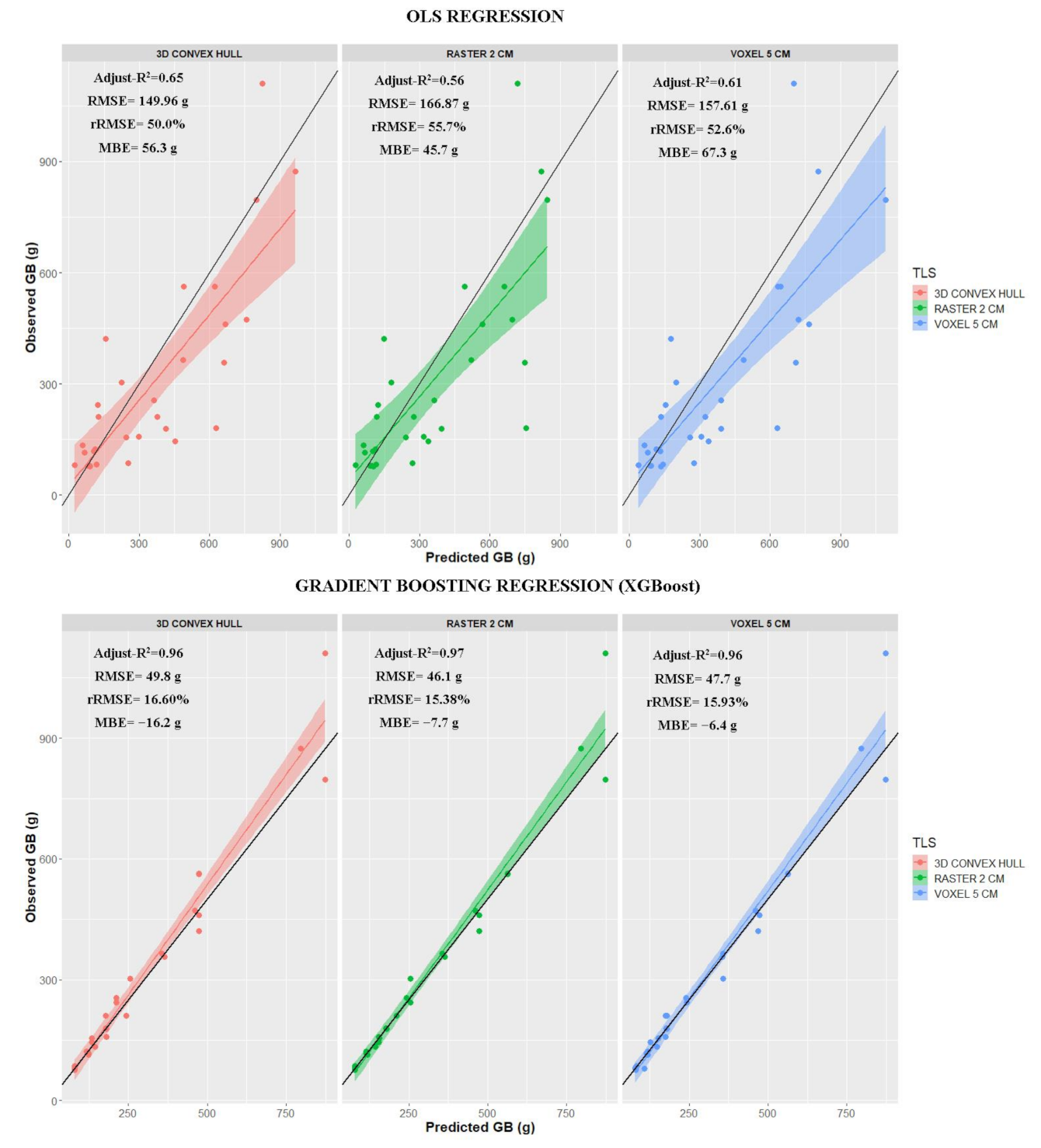
| TLS Method | Equation | Adjust-R2 | RMSE (g) | rRMSE (%) | MBE (g) |
|---|---|---|---|---|---|
| 3D Convex Hull | 1865.5 × TLS volume × (53.969 × NDVI − 1.940)/100 | 0.65 *** | 149.96 | 50.0 | 56.3 |
| Raster (2 cm) | 2472.1 × TLS volume × (53.969 × NDVI − 1.940)/100 | 0.56 *** | 166.87 | 55.7 | 45.7 |
| Voxel (5 cm) | 2416.8 × TLS volume × (53.969 × NDVI − 1.940)/100 | 0.61 *** | 157.61 | 52.6 | 67.3 |
Publisher’s Note: MDPI stays neutral with regard to jurisdictional claims in published maps and institutional affiliations. |
© 2021 by the authors. Licensee MDPI, Basel, Switzerland. This article is an open access article distributed under the terms and conditions of the Creative Commons Attribution (CC BY) license (https://creativecommons.org/licenses/by/4.0/).
Share and Cite
Rodríguez-Lozano, B.; Rodríguez-Caballero, E.; Maggioli, L.; Cantón, Y. Non-Destructive Biomass Estimation in Mediterranean Alpha Steppes: Improving Traditional Methods for Measuring Dry and Green Fractions by Combining Proximal Remote Sensing Tools. Remote Sens. 2021, 13, 2970. https://doi.org/10.3390/rs13152970
Rodríguez-Lozano B, Rodríguez-Caballero E, Maggioli L, Cantón Y. Non-Destructive Biomass Estimation in Mediterranean Alpha Steppes: Improving Traditional Methods for Measuring Dry and Green Fractions by Combining Proximal Remote Sensing Tools. Remote Sensing. 2021; 13(15):2970. https://doi.org/10.3390/rs13152970
Chicago/Turabian StyleRodríguez-Lozano, Borja, Emilio Rodríguez-Caballero, Lisa Maggioli, and Yolanda Cantón. 2021. "Non-Destructive Biomass Estimation in Mediterranean Alpha Steppes: Improving Traditional Methods for Measuring Dry and Green Fractions by Combining Proximal Remote Sensing Tools" Remote Sensing 13, no. 15: 2970. https://doi.org/10.3390/rs13152970
APA StyleRodríguez-Lozano, B., Rodríguez-Caballero, E., Maggioli, L., & Cantón, Y. (2021). Non-Destructive Biomass Estimation in Mediterranean Alpha Steppes: Improving Traditional Methods for Measuring Dry and Green Fractions by Combining Proximal Remote Sensing Tools. Remote Sensing, 13(15), 2970. https://doi.org/10.3390/rs13152970