Evaluating Signalization and Channelization Selections at Intersections Based on an Entropy Method


Abstract
1. Introduction
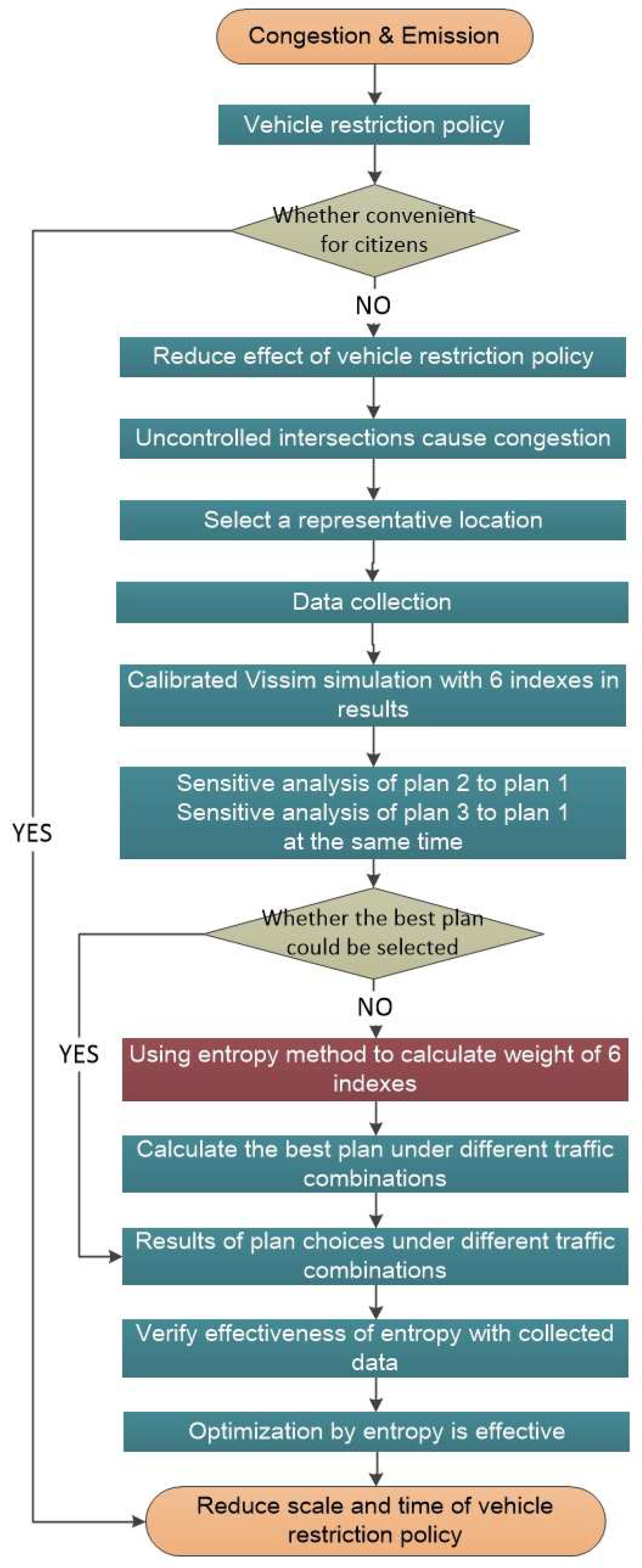
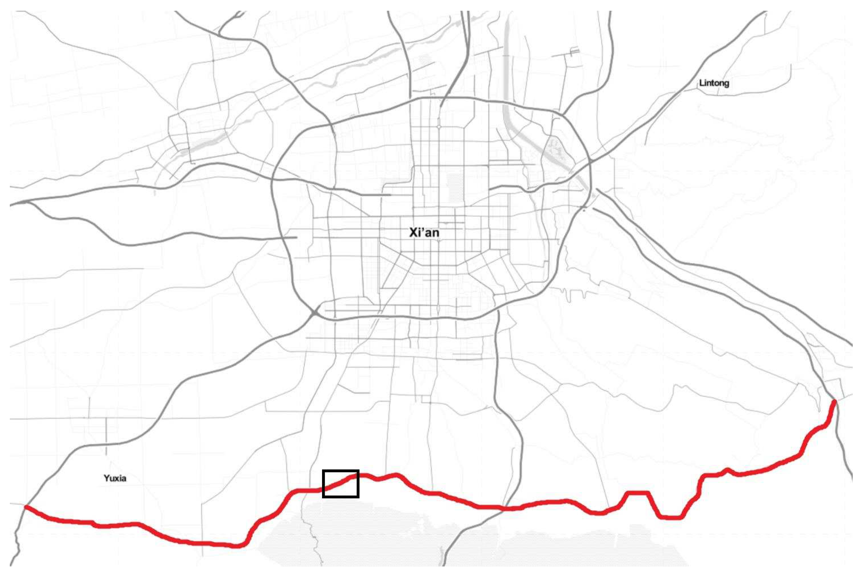
2. Problem Statement and Design Schemes
2.1. Problem Statement
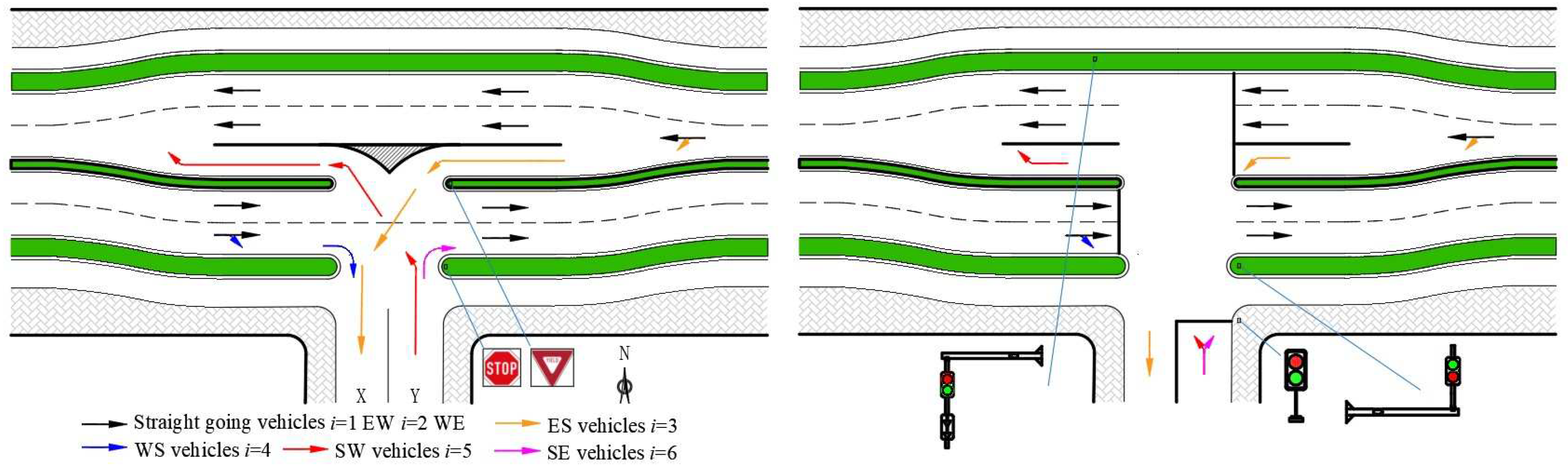
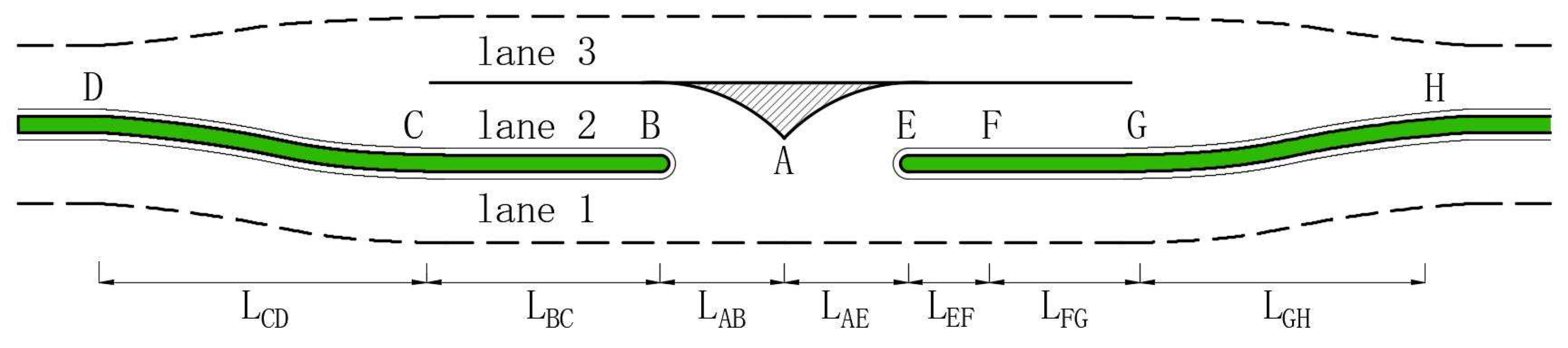
2.2. Design Scheme Description
3. Data Collection and VISSIM Simulation
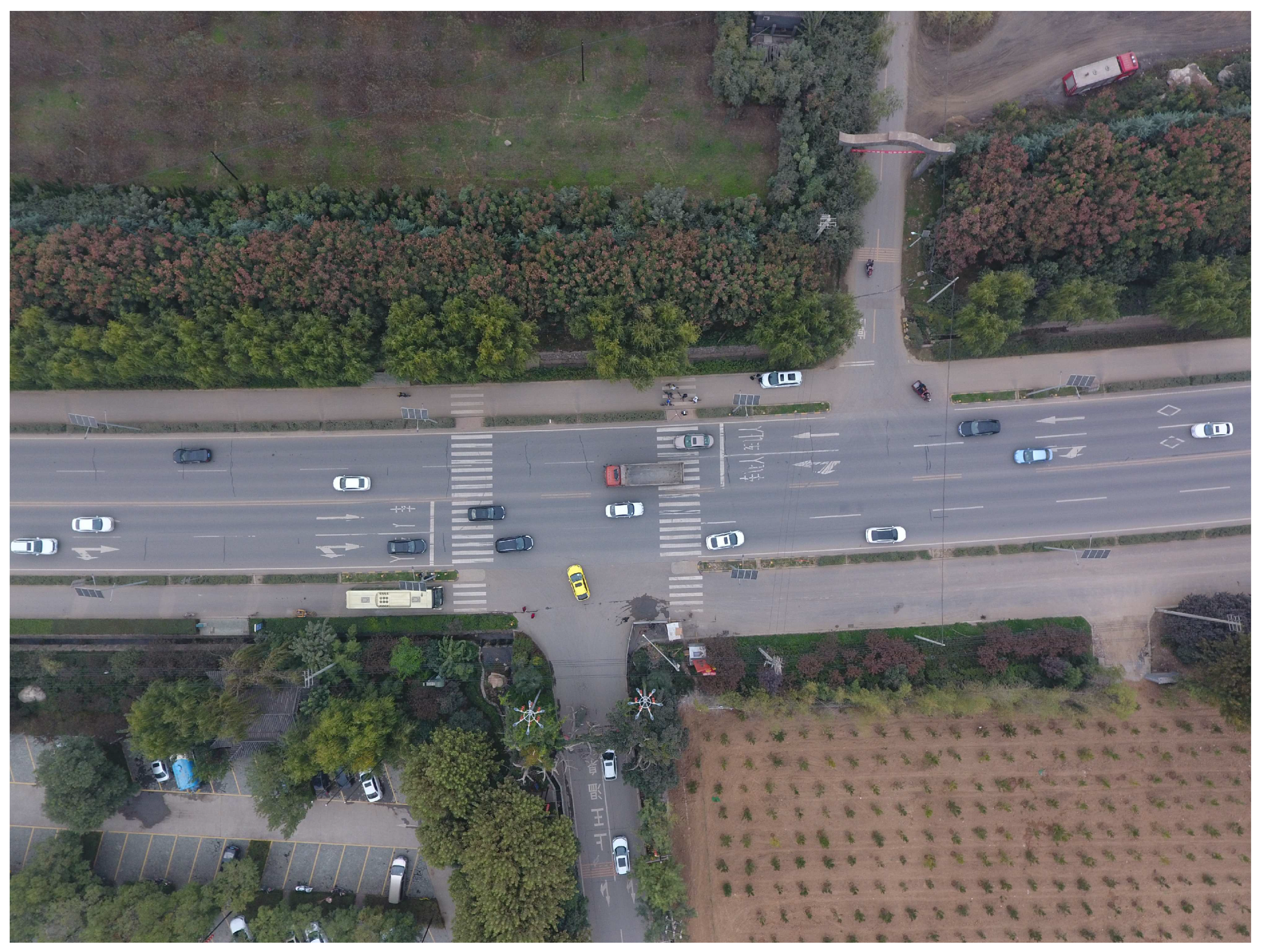
3.1. Data Collection
- Collect all vehicle speeds and types in each lane during collection period.
- Record every turning vehicle and type.
- Collect all vehicle trajectories.
- The majority of running speeds for flows were much lower than the speed limit and design speed (80 km/h).
- Flow was strongly influenced by TVs (flows ).
- Flow was influenced by TVs (flows ) but not as strongly as flow .
3.2. Calibration of VISSIM Simulation Model
- The percentages of large vehicles and cars are 4% and 96% in EW and 8% and 92% in WE, respectively.
- From west to east, the flow ratio is 8% and the flow ratio is 92%.
- From east to west, the flow ratio is 4% and the flow ratio is 96%.
- The flow ratio is 54% and flow ratio is 46% on the collector street.
- The headway of vehicles ranges from 1.5 to 15.1 s with an average of 6.9 s.
- Turning speed ranges from 0 to 28.5 km/h.
- The expectation speed is 25.2–81.4 km/h in EW and 0–91.4 km/h in WE.
3.3. Vissim Calculation of Operational Measures
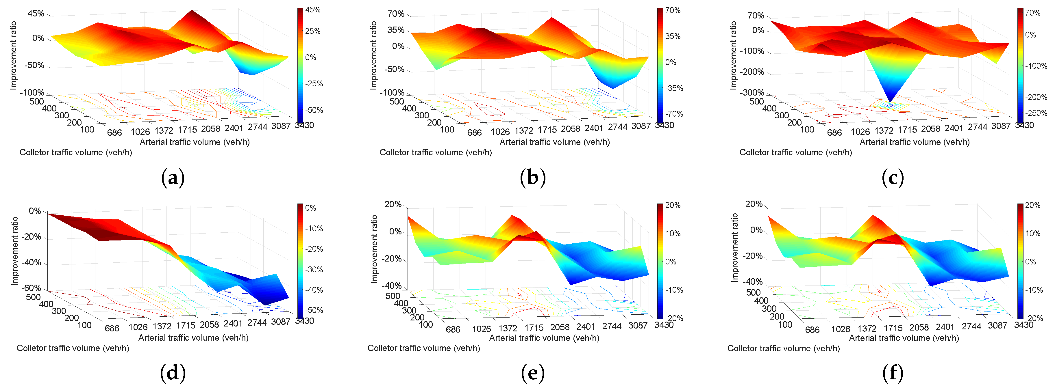
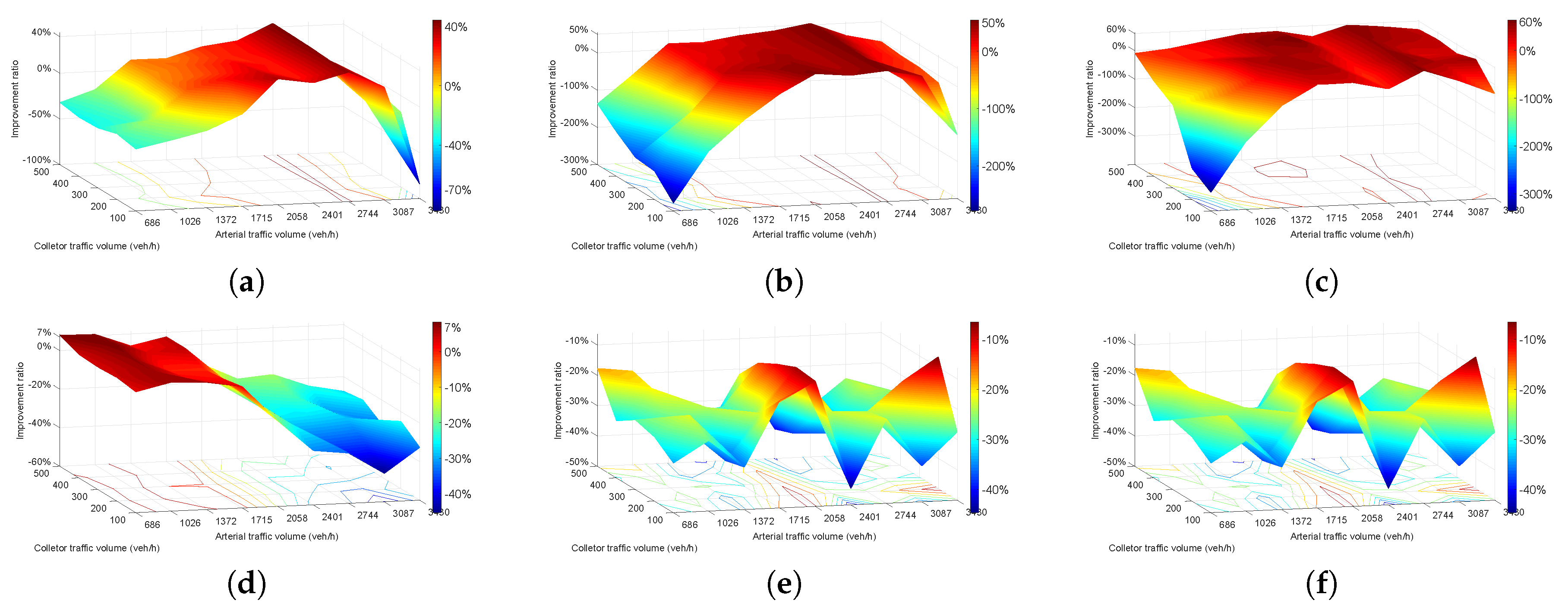
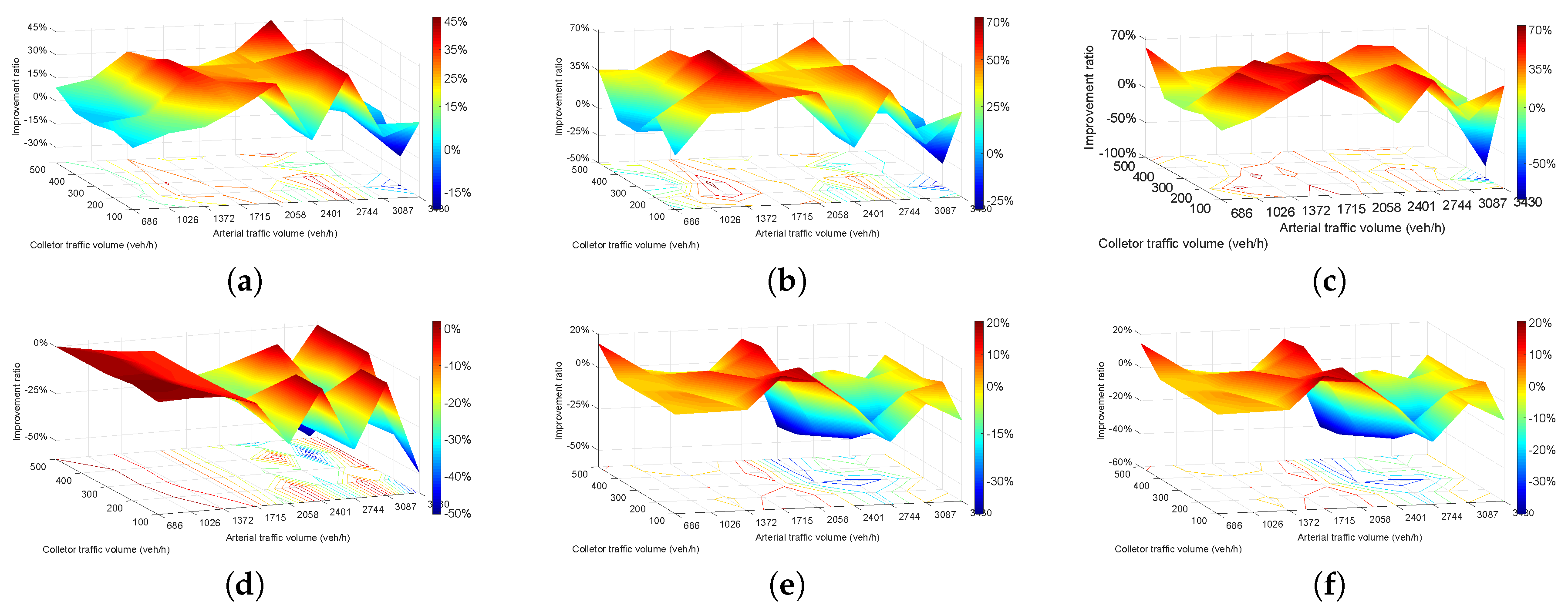
3.4. Sensitivity Analysis of Operational Performance
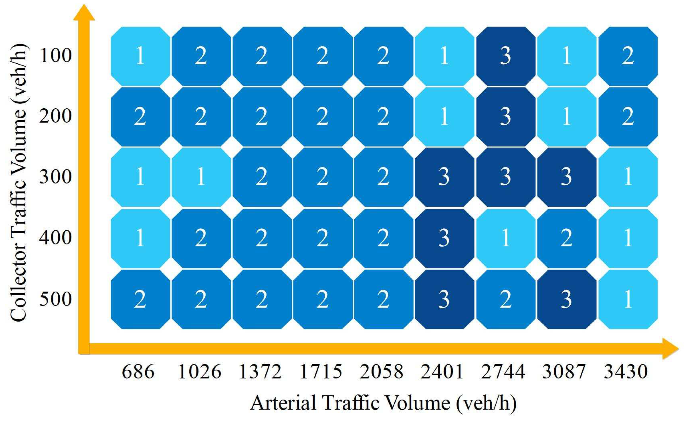
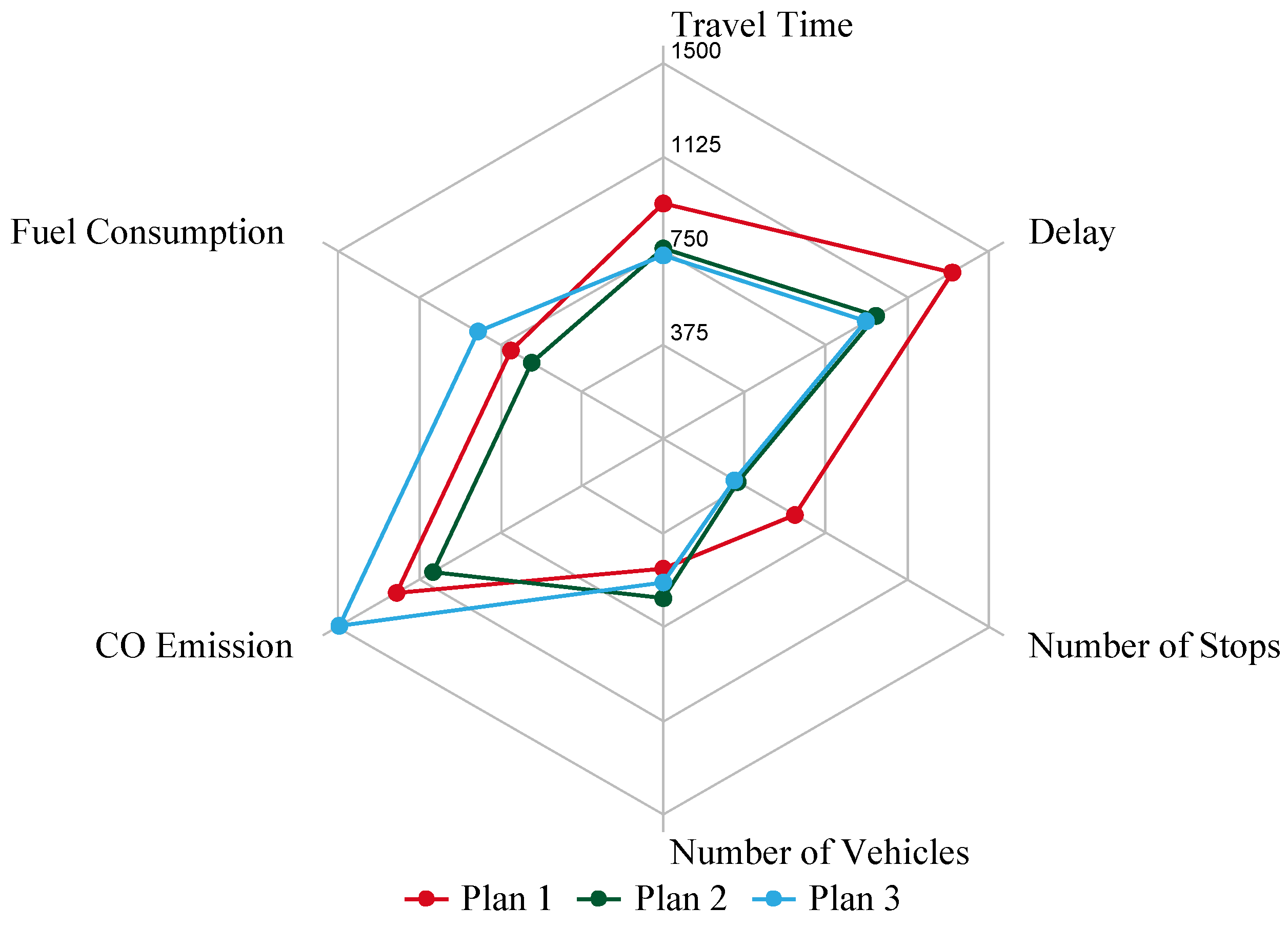
4. Results
Verifying the Validity of the EEM
5. Conclusions
Author Contributions
Funding
Acknowledgments
Conflicts of Interest
References
- Ma, C.X.; Hao, W.; Xiang, W.; Wei, Y. The Impact of Aggressive Driving Behavior on Driver-Injury Severity at Highway-Rail Grade Crossings Accidents. J. Adv. Transp. 2018, 2018, 9841498. [Google Scholar] [CrossRef]
- Vittorio, A.; Vincenzo, P.G. From traffic conflict simulation to traffic crash simulation: Introducing traffic safety indicators based on the explicit simulation of potential driver errors. Simul. Model. Pract. Theory 2019, 94, 215–236. [Google Scholar]
- Chen, J.X.; Wang, W.; Li, Z.B.; Jiang, H.; Chen, X.W.; Zhu, S.L. Dispersion effect in left-Turning bicycle traffic and its influence on capacity of left-turning vehicles at signalized intersections. Trans. Res. Rec. 2014, 2468, 38–46. [Google Scholar] [CrossRef]
- Autey, J.; Sayed, T.; Esawey, E.M. Guidelines for the use of some unconventional intersection designs. In Proceedings of the 4th International Symposium on Highway Geometric Design, Valencia, Spain, 2–5 June 2010. [Google Scholar]
- Reid, J.D.; Hummer, J.E. Travel Time Comparisons between Seven Unconventional Arterial Intersection Designs. Trans. Res. Rec. 2001, 1751, 56–66. [Google Scholar] [CrossRef]
- Zhao, J.; Ma, W.J.; Head, K.L.; Yang, X.G. Optimal Intersection Operation with Median U-Turn Lane-Based Approach. Trans. Res. Rec. 2014, 2439, 71–82. [Google Scholar] [CrossRef]
- Hummer, J.E.; Reid, J.E. Unconventional Left Turn Alternatives for Urban and Suburban Arterials-An Update. In Proceedings of the Transportation, Research Circular E-C019: Urban Street Symposium Conference Proceedings, Dallas, TX, USA, 28–30 June 1999; pp. 28–30. [Google Scholar]
- Ram, J.; Vanasse, H.B. Synthesis of the Median U-Turn Intersection Treatment, Safety, and Operational Benefits; Transportation Research Board: Washington, DC, USA, 2007. [Google Scholar]
- Kesting, A.; Treiber, M.; Schonhof, M.; Helbing, D. Adaptive cruise control design for active congestion avoidance. Trans. Res. Part C Emerg. Technol. 2008, 16, 668–683. [Google Scholar] [CrossRef]
- Maze, T.; Henderson, J.L.; Sankar, R. Impacts on Safety of Left-turn Treatment at High Speed Signalized Intersections; Project HR-347; Midwest Transportation Consortium: Ames, IA, USA, 1994. [Google Scholar]
- Brubacher, J.R.; Desapriya, E.; Chan, H.; Ranatunga, Y.; Harjee, R.; Erdelyi, S.; Asbridge, M.; Purssell, R.; Pike, I. Media reporting of traffic legislation changes in British Columbia (2010). Accid. Anal. Prev. 2015, 82, 227–233. [Google Scholar] [CrossRef]
- Carter, D.; Hummer, J.E.; Foyle, R.S.; Phillips, S. Operational and Safety Effects of U-turns at Signalized Intersections. Trans. Res. Rec. 2005, 1912, 11–18. [Google Scholar] [CrossRef]
- Zhou, H.G.; Lu, J.J.; Yang, X.K.; Dissanayake, S.; Williams, K.M. Operational effects of U-turns as alternatives to direct left turns from driveways. Trans. Res. Rec. 2002, 1796, 72–79. [Google Scholar] [CrossRef]
- Levinson, H.S.; Potts, I.B.; Harwood, D.W.; Gluck, J.; Torbic, D.J. Safety of U-turns at unsignalized median openings-Some research findings. Trans. Res. Rec. 2005, 1912, 72–81. [Google Scholar] [CrossRef]
- Wael, K.M.A.; Miho, A.; Hideki, N. Left-turn gap acceptance models considering pedestrian movement characteristics. Accid. Anal. Prev. 2013, 50, 175–185. [Google Scholar]
- Yang, X.K.; Zou, G.H. CORSIM-Based Simulation Approach to Evaluation of Direct Left Turn vs. Right Rurn Plus U-Turn from Driveways. J. Transp. Eng. 2004, 130, 68–75. [Google Scholar] [CrossRef]
- Topp, A.; Hummer, J.E. Comparison of Two Median U-Turn Design Alternatives Using Microscopic Simulation; Transportation Research Board: Washington, DC, USA, 2005. [Google Scholar]
- Liu, P.; Qu, X.; Yu, H.; Wang, W.; Gao, B. Development of a VISSIM simulation model for U-turns at unsignalized intersections. J. Transp. Eng. 2012, 138, 1333–1339. [Google Scholar] [CrossRef]
- Mesterton-Gibbons, M. Traffic flow at a T-junction: A sufficient condition for a left-turn lane. Math. Comput. Model. 1996, 24, 53–57. [Google Scholar] [CrossRef]
- Shao, Y.; Han, X.; Wu, H.; Shan, H.; Yang, S.; Claudel, C.G. Evaluating the sustainable traffic flow operational features of an exclusive spur dike U-turn lane design. PLoS ONE 2019, 14, e0214759. [Google Scholar] [CrossRef] [PubMed]
- Zhao, J.; Ma, W.; Head, K.L.; Yang, X.G. Optimal operation of displaced left-turn intersections: A lane-based approach. Trans. Res. Part C Emerg. Technol. 2015, 61, 29–48. [Google Scholar] [CrossRef]
- Do, G.K.; Simon, W. The significance of endogeneity problems in crash models: An examination of left-turn lanes in intersection crash models. Accid. Anal. Prev. 2006, 38, 1094–1100. [Google Scholar]
- Ma, W.J.; Liu, Y.; Zhao, J.; Wu, N. Increasing the capacity of signalized intersections with left-turn waiting areas. Transp. Res. Part A 2017, 105, 181–196. [Google Scholar] [CrossRef]
- Xuan, Y.G.; Carlos, F.D.; Michael, J.C. Increasing the capacity of signalized intersections with separate left turn phases. Transp. Res. Part B 2011, 45, 769–781. [Google Scholar] [CrossRef]
- Juraek, O.; Eungcheol, K.; Myungseob, K.; Choo, S. Development of conflict techniques for left-turn and cross-traffic at protected left-turn signalized intersections. Saf. Sci. 2010, 48, 460–468. [Google Scholar]
- Nikiforos, S.; Adam, H.; Adam, K. A simulation-based approach in determining permitted left-turn capacities. Trans. Res. Part C Emerg. Technol. 2015, 55, 486–495. [Google Scholar]
- Wu, J.M.; Liu, P.; Tian, Z.Z.; Xu, C.C. Operational analysis of the contraflow left-turn lane design at signalized intersections in China. Trans. Res. Part C Emerg. Technol. 2016, 69, 228–241. [Google Scholar] [CrossRef]
- Ma, C.X.; Hao, W.; Wang, A.B.; Zhao, H.X. Developing a Coordinated Signal Control System for Urban Ring Road under the Vehicle-infrastructure Connected Environment. IEEE Access 2018, 6, 52471–52478. [Google Scholar] [CrossRef]
- Yan, X.D.; Essam, R.; Guo, D.H. Effects of major-road vehicle speed and driver age and gender on left-turn gap acceptance. Accid. Anal. Prev. 2007, 39, 843–852. [Google Scholar] [CrossRef] [PubMed]
- Moussa, G.; Radwan, E.; Hussain, K. Augmented Reality Vehicle system: Left-turn maneuver study. Trans. Res. Part C Emerg. Technol. 2012, 21, 1–16. [Google Scholar] [CrossRef]
- Azuma, R.T. A survey of augmented reality. Teleoper. Virtual Environ. 1997, 6, 355–385. [Google Scholar] [CrossRef]
- Grega, J.; Christina, D.; Jaka, S. A user study of auditory, head-up and multi-modal displays in vehicles. Appl. Ergon. 2015, 46, 184–192. [Google Scholar]
- Wuryandari, A.I.; Gondokaryono, Y.S.; Widnyana, I.M.Y. Design and Implementation of Driver Main Computer and Head up Display on Smart Car. Procedia Technol. 2013, 11, 1041–1047. [Google Scholar] [CrossRef][Green Version]
- Liu, Y.; Dong, H.W.; Zhang, L.Y.; EI Saddik, A. Technical Evaluation of HoloLens for Multimedia: A First, Look. IEEE Multimed. 2018, 25, 8–18. [Google Scholar] [CrossRef]
- Huang, J.; Shang, Y.Y.; Chen, H. Improved Viola-Jones face detection algorithm based on HoloLens. EURASIP J. Image Video Process. 2019, 2019, 41. [Google Scholar] [CrossRef]
- Fragkias, M.; Lobo, J.; Strumsky, D.; Seto, K.C. Does Size Matter? Scaling of CO2 Emissions and U.S. Urban Areas. PLoS ONE 2013, 8, e64727. [Google Scholar] [CrossRef] [PubMed]
- Huseynov, S.; Palma, M.A. Does California’s Low Carbon Fuel Standards reduce carbon dioxide emissions? PLoS ONE 2018, 13, e0203167. [Google Scholar] [CrossRef] [PubMed]
- Li, X.; Yang, T.; Liu, J.; Qin, X.; Yu, S. Effects of vehicle gap changes on fuel economy and emission performance of the traffic flow in the ACC strategy. PLoS ONE 2018, 13, e0200110. [Google Scholar] [CrossRef] [PubMed]
- Lin, C.; Gong, B.; Qu, X. Low Emissions and Delay Optimization for an Isolated Signalized Intersection Based on Vehicular Trajectories. PLoS ONE 2015, 10, e0146018. [Google Scholar] [CrossRef] [PubMed]
- Meneguette, R.I.; Filho, G.P.R.; Guidoni, D.L.; Pessin, G.; Villas, L.A.; Jo, U. Increasing Intelligence in Inter-Vehicle Communications to Reduce Traffic Congestions: Experiments in Urban and Highway Environments. PLoS ONE 2016, 11, e0159110. [Google Scholar] [CrossRef] [PubMed]
- Li, J.J.; Li, X.B.; Li, B.; Peng, Z.R. The Effect of Nonlocal Vehicle Restriction Policy on Air Quality in Shanghai. Atmosphere 2018, 9, 299. [Google Scholar] [CrossRef]
- Tang, C.; Ceder, A.; Ge, Y.E. Optimal public-transport operational strategies to reduce cost and vehicle’s emission. PLoS ONE 2018, 13, e0201138. [Google Scholar] [CrossRef] [PubMed]
- Liu, Z.Y.; Li, R.M.; Wang, X.K.; Shang, P. Effects of vehicle restriction policies: Analysis using license plate recognition data in Langfang, China. Transp. Res. Part A Policy Pract. 2018, 118, 89–103. [Google Scholar] [CrossRef]
- Li, P.H.; Steven, J. Vehicle restrictions and CO2 emissions in Beijing—A simple projection using available data. Transp. Res. Part D 2015, 41, 467–476. [Google Scholar] [CrossRef]
- Zhang, L.L.; Long, R.Y.; Chen, H. Do car restriction policies effectively promote the development of public transport? World Dev. 2019, 119, 100–110. [Google Scholar] [CrossRef]
- Yang, Q.L.; Shi, Z.K.; Yu, S.W.; Zhou, J. Analytical evaluation of the use of left-turn phasing for single left-turn lane only. Transp. Res. Part B 2018, 111, 266–303. [Google Scholar] [CrossRef]
- Per-Olof, P. A sparse and high-order accurate line-based discontinuous Galerkin method for unstructured meshes. J. Comput. Phys. 2013, 233, 414–429. [Google Scholar]
- Jiang, W.; Hu, W.W. An improved soft likelihood function for Dempster-Shafer belief structures. Int. J. Intell. Syst. 2018, 33, 1264–1282. [Google Scholar] [CrossRef]
- Cao, Z.H.; Lin, C.T. Inherent Fuzzy Entropy for the Improvement of EEG Complexity Evaluation. IEEE Trans. Fuzzy Syst. 2018, 26, 1032–1035. [Google Scholar] [CrossRef]
- El-Yaagoubi, M.; Goya-Esteban, R.; Jabrane, Y.; Muñoz-Romero, S.; García-Alberola, A.; Rojo-Álvarez, J.L. On the Robustness of Multiscale Indices for Long-Term Monitoring in Cardiac Signals. Entropy 2019, 21, 594. [Google Scholar] [CrossRef]
- Tian, Z.P.; Wang, J.Q.; Zhang, H.Y. An integrated approach for failure mode and effects analysis based on fuzzy best-worst, relative entropy, and VIKOR methods. Appl. Soft Comput. 2018, 72, 636–646. [Google Scholar] [CrossRef]
- Chen, W.; Li, H.; Wang, S.Q.; Wang, G.R.; Panahi, M.; Li, T.; Peng, T.; Guo, C.; Niu, C.; Xiao, L.; et al. GIS-based groundwater potential analysis using novel ensemble weights-of-evidence with logistic regression and functional tree models. Sci. Total Environ. 2018, 634, 853–867. [Google Scholar] [CrossRef] [PubMed]
- Dávalos, A.; Jabloun, M.; Ravier, P.; Buttelli, O. On the Statistical Properties of Multiscale Permutation Entropy: Characterization of the Estimator’s Variance. Entropy 2019, 21, 450. [Google Scholar] [CrossRef]
- Zhao, X.; Liang, C.; Zhang, N.; Shang, P. Quantifying the Multiscale Predictability of Financial Time Series by an Information-Theoretic Approach. Entropy 2019, 21, 684. [Google Scholar] [CrossRef]
- Shang, H.; Li, F.; Wu, Y. Partial Discharge Fault Diagnosis Based on Multi-Scale Dispersion Entropy and a Hypersphere Multiclass Support Vector Machine. Entropy 2019, 21, 81. [Google Scholar] [CrossRef]
- Xu, C.; Xu, C.; Tian, W.; Hu, A.; Jiang, R. Multiscale Entropy Analysis of Page Views: A Case Study of Wikipedia. Entropy 2019, 21, 229. [Google Scholar] [CrossRef]
- Department of Xi’an Police. 2018 Xi’an Vehicle Ownership Report; Department of Xi’an Police: Xi’an, China, 2019.
- Xi’an Municipal Bureau of Statistics. 2018 Xi’an Statistical Yearbook; Xi’an Municipal Bureau of Statistics: Xi’an, China, 2019.
- American Association of State and Highway Transportation Officials (AASHTO). Highway Capacity Manual, 6th ed.; AASHTO: Washington, DC, USA, 2010. [Google Scholar]
- American Association of State and Highway Transportation Officials (AASHTO). A Policy on Geometric Design of Highways and Streets, 6th ed.; AASHTO: Washington, DC, USA, 2011. [Google Scholar]
- Ashraf, M.I.; Sinha, S. The handedness of language: Directional symmetry breaking of sign usage in words. PLoS ONE 2018, 13, e0190735. [Google Scholar] [CrossRef] [PubMed]
- Lu, A.T.; Yu, Y.P.; Niu, J.X.; Zhang, J.X. The Effect of Sign Language Structure on Complex Word Reading in Chinese Deaf Adolescents. PLoS ONE 2015, 10, e0120943. [Google Scholar] [CrossRef] [PubMed]
- Pijoan, A.; Kamara-Esteban, O.; Alonso-Vicario, A.; Borges, C.E. Transport Choice Modeling for the Evaluation of New Transport Policies. Sustainability 2018, 10, 1230. [Google Scholar] [CrossRef]
- Wang, J.H.; Kong, Y.M.; Fu, T.; Stipancic, J. The impact of vehicle moving violations and freeway traffic flow on crash risk: An application of plugin development for microsimulation. PLoS ONE 2017, 12, e0184564. [Google Scholar] [CrossRef] [PubMed]
- Gupta, A.K.; Dhiman, I. Analyses of a continuum traffic flow model for a nonlane-based system. Int. J. Modern Phys. C 2014, 25, 1450045. [Google Scholar] [CrossRef]
- Chen, H.; Zhang, N.; Qian, Z.D. VISSIM-Based Simulation of the Left-Turn Waiting Zone at Signalized Intersection. In Proceedings of the International Conference on Intelligent Computation Technology and Automation, Hunan, China, 20–22 October 2008; Volume 1. [Google Scholar]
- Tang, T.Q.; Wang, Y.P.; Yang, X.B.; Huang, H.J. A multilane traffic flow model accounting for lane width, lanechanging and the number of lanes. Netw. Spat. Econ. 2014, 14, 465–483. [Google Scholar] [CrossRef]
- Leng, J.Q.; Zhang, Y.P.; Sun, M.Q. VISSIM-Based Simulation Approach to Evaluation of Design and Operational Performance of U-turn at Intersection in China. In Proceedings of the WMSO: 2008 International Workshop on Modelling, Simulation and Optimization, Hong Kong, China, 27–28 December 2009. [Google Scholar]
- PTV, AG. PTV VISSIM 10 User Manual; PTV AG: Karlsruhe, Germany, 2018. [Google Scholar]
- Pan, F.Q.; Zhang, L.X.; Lu, J.; Zhao, J.J.; Wang, F.Y. A method for determining the number of traffic conflict points between vehicles at majorminor highway intersections. Traffic Inj. Prev. 2013, 14, 424–433. [Google Scholar] [CrossRef] [PubMed]
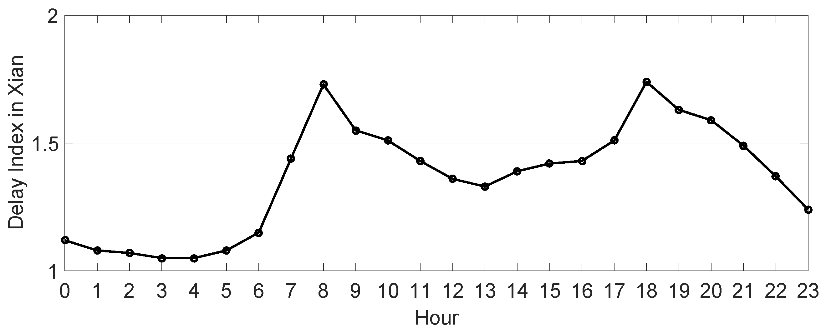
- AutoNavi Traffic Big-Data. 2017 Traffic Analysis Reports for Major Cities in China. 2018. Available online: https://report.amap.com/share.do?id=8a38bb86614afa0801614b0a029a2f79 (accessed on 18 January 2018).
- AutoNavi Traffic Big-Data. Xi’an Realtime Traffic Congestion Delay Index. Available online: https://report.amap.com/detail.do?city=610100 (accessed on 13 October 2018).
- Zhao, Y.; Liu, P.; Chen, Y.G.; Hao, Y. Can Left-turn Waiting Areas Improve the Capacity of Left-turn Lanes at Signalized Intersections? Procedia-Soc. Behav. Sci. 2012, 43, 192–200. [Google Scholar]
- Ronald, T.M.; Fred, C. Recommended guidelines for the calibration and validation of traffic simulation models. In Proceedings of the 8th TRB Conference on the Application of Transportation Planning, Methods, TX, USA, 22–26 April 2002; pp. 178–187. [Google Scholar]
- Park, B.; Won, J.; Yun, I. Application of Microscopic Simulation Model Calibration and Validation Procedure: Case Study of Coordinated Actuated Signal System. Traffic Signal Syst. Reg. Syst. Manag. 2006, 1978, 113–122. [Google Scholar] [CrossRef]
- Chu, L.Y.; Liu, H.; Oh, J.S.; Recker, W. A calibration procedure for microscopic traffic simulation. In Proceedings of the 2003 IEEE International Conference on Intelligent Transportation Systems, Shanghai, China, 12–15 October 2003; Volume 2, pp. 1574–1579. [Google Scholar]
- Xiang, Y.; Li, Z.; Wang, W.; Chen, J.; Wang, H.; Li, Y. Evaluating the Operational Features of an Unconventional Dual-Bay U-Turn Design for Intersections. PLoS ONE 2016, 11, e0163758. [Google Scholar] [CrossRef] [PubMed]
- Sun, J. Guideline for Microscopic Traffic Simulation Analysis; Tongji University Press: Shanghai, China, 2014. [Google Scholar]
- Jayasooriya, N.; Bandara, S. Calibrating and validating VISSIM microscopic simulation software for the context of Sri Lanka. In Proceedings of the 2018 Moratuwa Engineering Research Conference (MERCon), Moratuwa, Sri Lanka, 30 May–1 June 2018; pp. 494–499. [Google Scholar]
- Henclewood, D.; Suh, W.; Rodgers, M.O.; Fujimoto, R.; Hunter, M.P. A calibration procedure for increasing the accuracy of microscopic traffic simulation models. Simul. Trans. Soc. Model. Simul. Int. 2017, 93, 35–47. [Google Scholar] [CrossRef]
- Wang, J.Y.; Mao, Y.; Li, J.; Xiong, Z.; Wang, W.X. Predictability of Road Traffic and Congestion in Urban Areas. PLoS ONE 2015, 10, e0121825. [Google Scholar] [CrossRef] [PubMed]
- Ji, C.W.; Yu, M.H.; Wang, S.F.; Zhang, B.; Cong, X.Y.; Feng, Y.; Lin, S. The optimization of on-board H2 generator control strategy and fuel consumption of an engine under the NEDC condition with start-stop system and H2 start. Int. J. Hydrog. Energy 2016, 41, 19256–19264. [Google Scholar] [CrossRef]
- Natalia, F.; Jesus, C.; Manuel, V. Influence of the stop/start system on CO2 emissions of a diesel vehicle in urban traffic. Transp. Res. Part D Transp. Environ. 2011, 16, 194–200. [Google Scholar]


| Cities | Monday | Tuesday | Wednesday | Thursday | Friday | Note |
|---|---|---|---|---|---|---|
| Xi’an/Chengdu | 1, 6 | 2, 7 | 3, 8 | 4, 9 | 5, 0 | 07:00–20:00 |
| Beijing | 0, 5 | 1, 6 | 2, 7 | 3,8 | 4, 9 | The number changes every 3 months |
| Shanghai | Vehicles from other provinces all forbidden on weekdays | |||||
| Guangzhou | Drive consecutively for 4 days at most, stop driving for 4 days consecutively | |||||
| Item | Description |
|---|---|
| & | Symmetry design, 12.15 m length, radius is 22.5 m. Entrance and/or exit of ELTL for flow to turn |
| 190 m. Acceleration length for flow to accelerate to design speed | |
| 132 m. Length for seeking a headway for flow and merging into flow | |
| 27 m. Wait area length in case of flow needing to wait to turn | |
| 90 m. Deceleration length for flow from design speed to stop | |
| 50 m. Length of diversion to separate flow and flow |
| Time | Friday | Saturday |
|---|---|---|
| Morning | 2031 | 1944 |
| Middle noon | 1530 | 1836 |
| Evening | 2195 | 2240 |
| Item | East to West | West to East | Collector Street | |||
|---|---|---|---|---|---|---|
| Flow | ||||||
| Car | 920 | 40 | 898 | 80 | 108 | 92 |
| Truck/Bus | 50 | 0 | 52 | 0 | 0 | 0 |
| Average speed (km/h) | 45.5 | 16.7 | 37.3 | 11.5 | 18.4 | 8.5 |
| Max. speed (km/h) | 81.4 | 23.5 | 91.4 | 25.7 | 28.5 | 12.3 |
| Min. speed (km/h) | 25.2 | 0 | 0 | 0 | 0 | 0 |
| Flow | i = 1 | i = 2 | i = 3 | i = 4 | i = 5 | i = 6 |
|---|---|---|---|---|---|---|
| Investigated capacity (veh/h) | 970 | 950 | 40 | 80 | 108 | 92 |
| Simulated capacity (veh/h) | 936 | 864 | 50 | 90 | 90 | 108 |
| Individual MAPE | 3.5 | 9.0 | 25.0 | 12.5 | 16.7 | 17.4 |
| MAPE | 4.3 | |||||
| Index | T | D | S | V | C | F | Summation |
|---|---|---|---|---|---|---|---|
| Weight | 0.1727 | 0.1670 | 0.1262 | 0.1025 | 0.2158 | 0.2158 | 1.0000 |
© 2019 by the authors. Licensee MDPI, Basel, Switzerland. This article is an open access article distributed under the terms and conditions of the Creative Commons Attribution (CC BY) license (http://creativecommons.org/licenses/by/4.0/).
Share and Cite
Shao, Y.; Han, X.; Wu, H.; G. Claudel, C. Evaluating Signalization and Channelization Selections at Intersections Based on an Entropy Method. Entropy 2019, 21, 808. https://doi.org/10.3390/e21080808
Shao Y, Han X, Wu H, G. Claudel C. Evaluating Signalization and Channelization Selections at Intersections Based on an Entropy Method. Entropy. 2019; 21(8):808. https://doi.org/10.3390/e21080808
Chicago/Turabian StyleShao, Yang, Xueyan Han, Huan Wu, and Christian G. Claudel. 2019. "Evaluating Signalization and Channelization Selections at Intersections Based on an Entropy Method" Entropy 21, no. 8: 808. https://doi.org/10.3390/e21080808
APA StyleShao, Y., Han, X., Wu, H., & G. Claudel, C. (2019). Evaluating Signalization and Channelization Selections at Intersections Based on an Entropy Method. Entropy, 21(8), 808. https://doi.org/10.3390/e21080808