
Automatic Epileptic Seizure Detection in EEG Signals Using Multi-Domain Feature Extraction and Nonlinear Analysis

 ,
,
Abstract
:1. Introduction
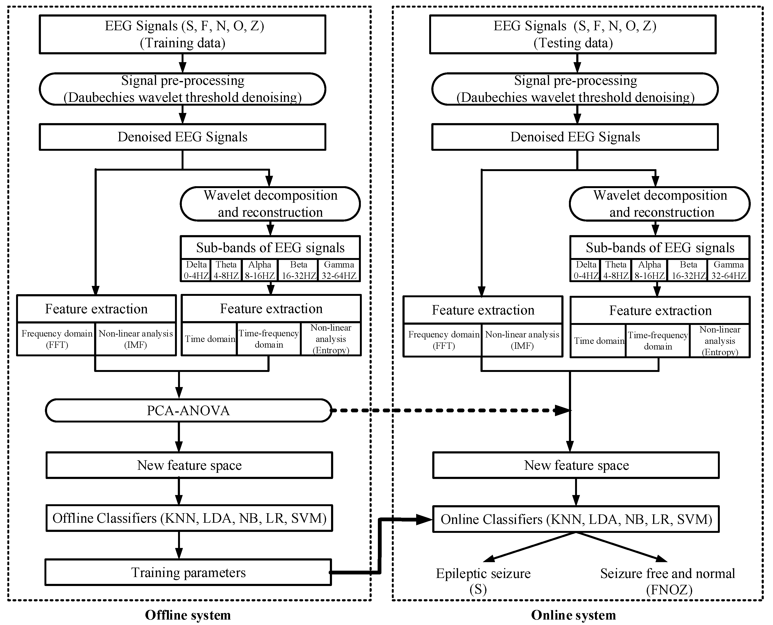
2. Methodology
2.1. Materials
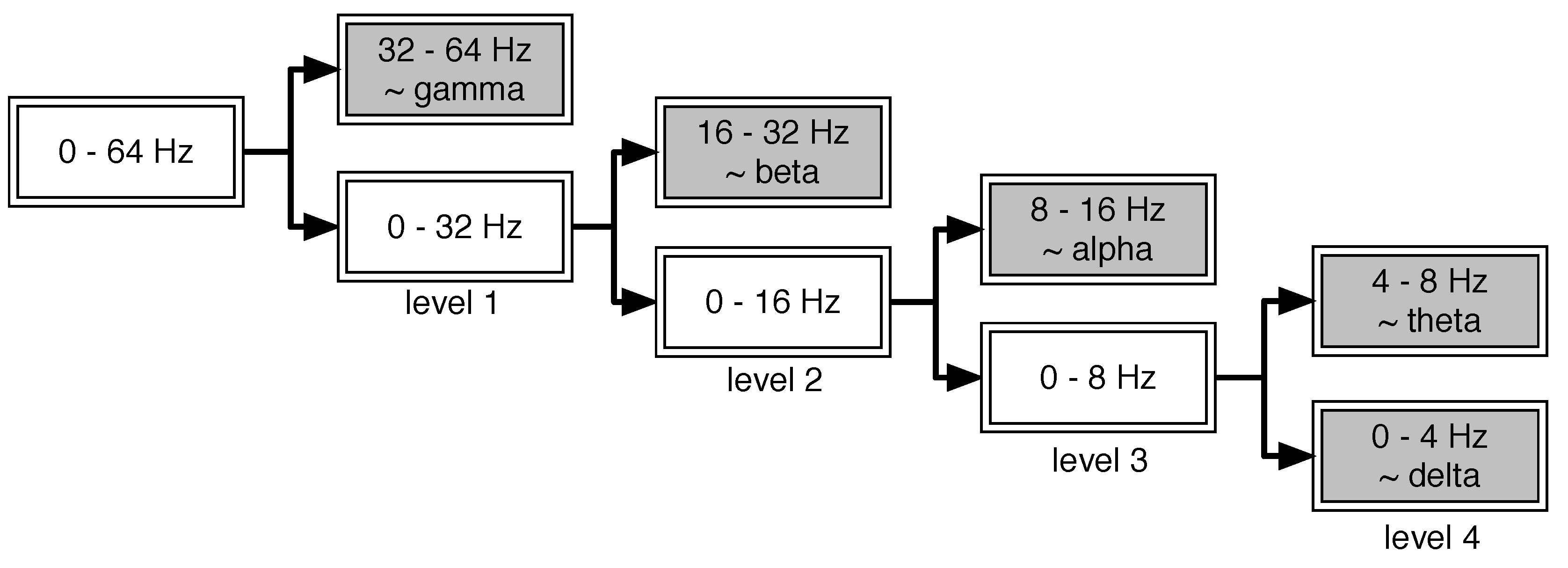
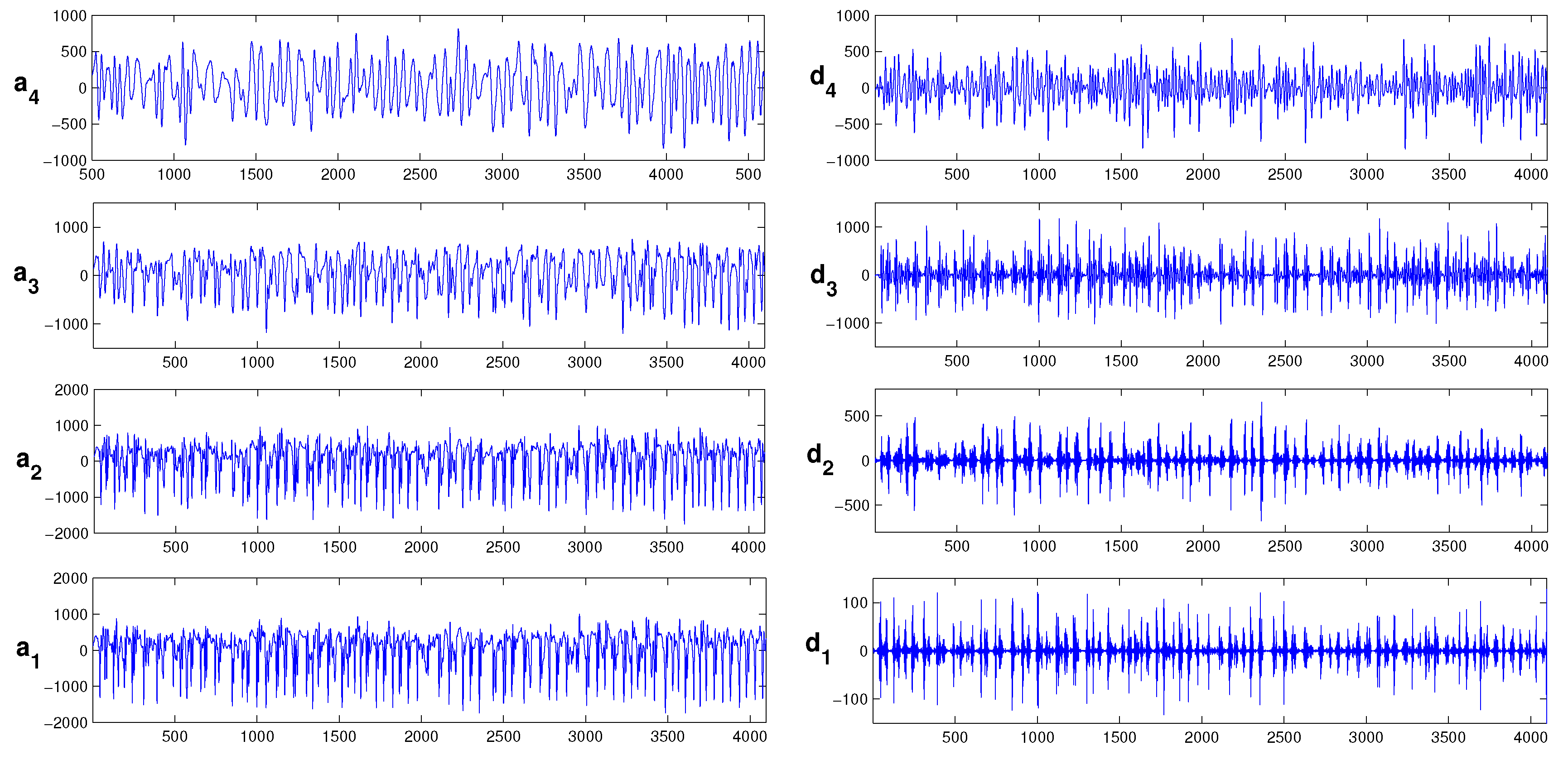
2.2. Signal Pre-Processing: Wavelet Threshold De-Noising
2.3. Feature Extraction
2.3.1. Feature Extraction in the Time Domain, Frequency Domain and Time-Frequency Domain
2.3.2. Feature Extraction via Nonlinear Analysis
- Procedure 1, IMF extraction procedure:
- Extract local max and local min magnitudes from signal ;
- Obtain the envelope by connecting all of the maximums with cubic spline interpolation, and similarly obtain the envelope by connecting all of the minimums with cubic spline interpolation;
- Compute the average of and , and denote as :
- Extract the detail from as:
- Check whether the detail satisfy the above conditions mentioned for IMF or not;
- Repeat Steps 1–5, until satisfies the conditions for IMF.
- Procedure 2, approximate entropy calculation:
- Let the values containing N samples in each sub-band be ;
- Let be a sub-sequence of X such that for , where m is the length of the sub-sequence;
- Let r represent the noise filter level that is defined as [33]:where SD is the standard deviation of the data sequence X.
- Let represent a set of sub-sequences obtained from by varying j from 1–(). Each sequence in the set of is compared with , and in this process, two parameters, namely and , are defined as follows:
- The approximate entropy is calculated by using and as follows:
2.4. Classification and Performance Evaluation
3. Results
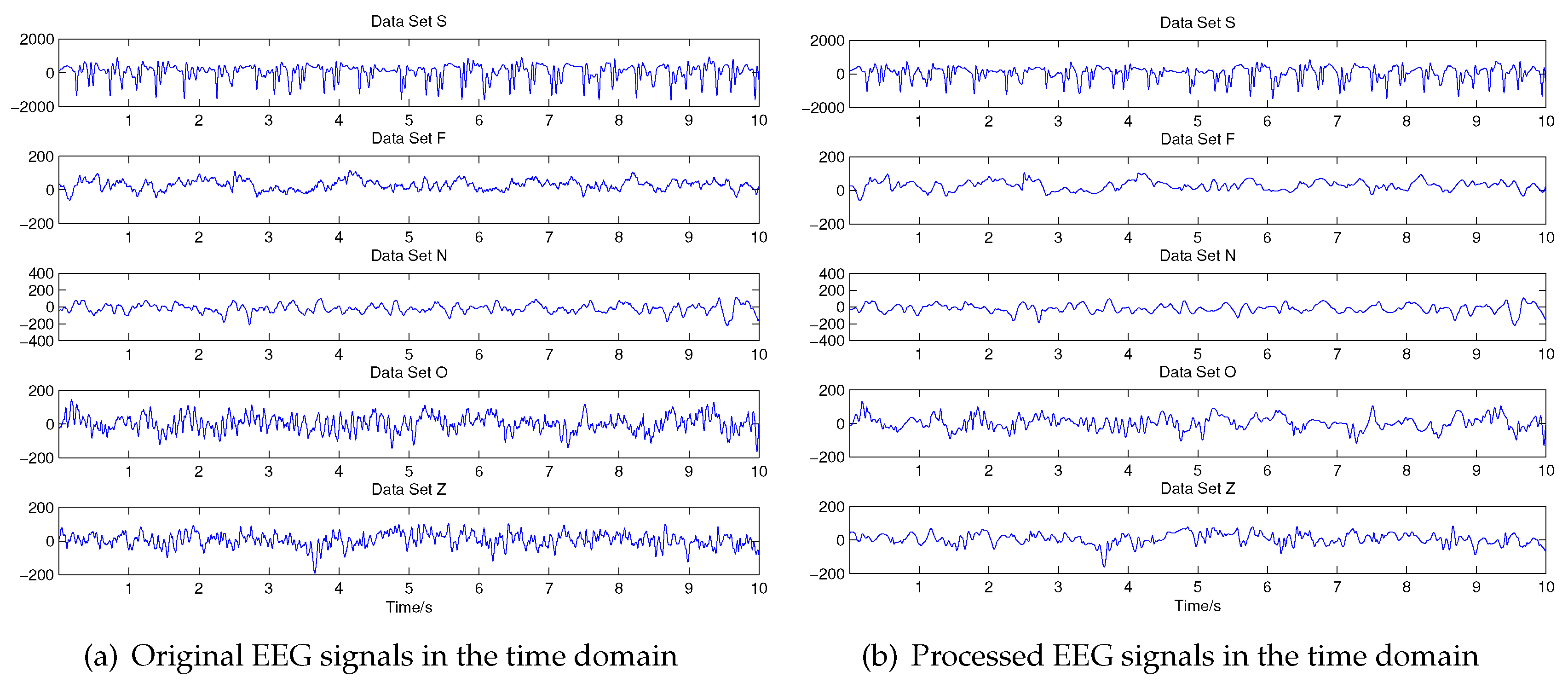
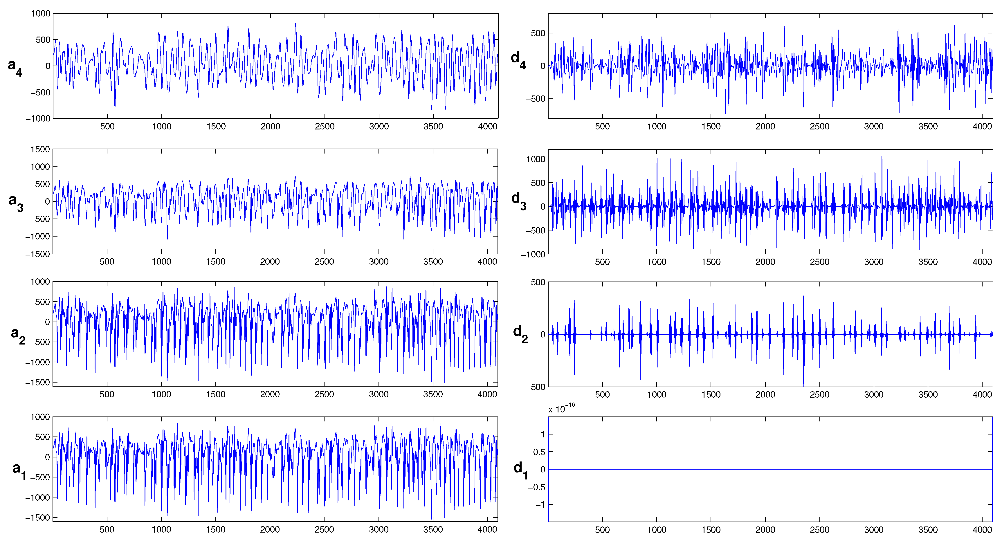
3.1. Wavelet Threshold Denoising and Feature Extraction
3.2. Dimension Reduction in Feature Space
3.3. Experiment Classification Results
4. Discussion and Conclusions
Acknowledgments
Author Contributions
Conflicts of Interest
References
- Acharya, U.R.; Sree, S.V.; Alvin, A.P.C.; Yanti, R.; Suri, J.S. Application of non-linear and wavelet based features for the automated identification of epileptic eeg signals. Int. J. Neural Syst. 2012, 22, 1250002. [Google Scholar] [CrossRef] [PubMed]
- Mormann, F.; Andrzejak, R.G.; Elger, C.E.; Lehnertz, K. Seizure prediction: The long and winding road. Brain 2007, 130, 314–333. [Google Scholar] [CrossRef] [PubMed]
- Tzallas, A.T.; Tsipouras, M.G.; Fotiadis, D.I. Automatic seizure detection based on time-frequency analysis and artificial neural networks. Comput. Int. Neurosci. 2007, 2007, 1–13. [Google Scholar] [CrossRef] [PubMed]
- Hassan, A.R.; Siuly, S.; Zhang, Y. Epileptic seizure detection in eeg signals using tunable-q factor wavelet transform and bootstrap aggregating. Comput. Methods Progr. Biomed. 2016, 137, 247–259. [Google Scholar] [CrossRef] [PubMed]
- Rizvi, S.A.; Zenteno, J.F.T.; Crawford, S.L.; Wu, A. Outpatient ambulatory eeg as an option for epilepsy surgery evaluation instead of inpatient eeg telemetry. Epilepsy Behav. Case Rep. 2013, 1, 39–41. [Google Scholar] [CrossRef] [PubMed]
- Li, Y.; Wei, H.L.; Billings, S.A.; Liao, X.F. Time-varying linear and nonlinear parametric model for granger causality analysis. Phys. Rev. E 2012, 85, 041906. [Google Scholar] [CrossRef] [PubMed]
- Ocak, H. Automatic detection of epileptic seizures in eeg using discrete wavelet transform and approximate entropy. Expert Syst. Appl. 2009, 36, 2027–2036. [Google Scholar] [CrossRef]
- Tzallas, A.T.; Tsipouras, M.G.; Fotiadis, D.I. Epileptic seizure detection in eegs using time-frequency analysis. IEEE Trans. Inf. Technol. Biomed. 2009, 13, 703–710. [Google Scholar] [CrossRef] [PubMed]
- Guo, L.; Rivero, D.; Dorado, J.; Munteanu, C.R.; Pazos, A. Automatic feature extraction using genetic programming: An application to epileptic eeg classification. Expert Syst. Appl. 2011, 38, 10425–10436. [Google Scholar] [CrossRef]
- Fu, K.; Qu, J.F.; Chai, Y.; Zou, T. Hilbert marginal spectrum analysis for automatic seizure detection in eeg signals. Biomed. Signal Process. Control 2015, 18, 179–185. [Google Scholar] [CrossRef]
- Lee, S.H.; Lim, J.S.; Kim, J.K.; Yang, J.; Lee, Y. Classification of normal and epileptic seizure eeg signals using wavelet transform, phase-space reconstruction, and euclidean distance. Comput. Methods Progr. Biomed. 2014, 116, 10–25. [Google Scholar] [CrossRef] [PubMed]
- Polat, K.; Güne, S. Classification of epileptiform eeg using a hybrid system based on decision tree classifier and fast fourier transform. Appl. Math. Comput. 2007, 187, 1017–1026. [Google Scholar] [CrossRef]
- Li, Y.; Liu, Q.; Tan, S.R.; Chan, R.H.M. High-resolution time-frequency analysis of eeg signals using multiscale radial basis functions. Neurocomputing 2016, 195, 96–103. [Google Scholar] [CrossRef]
- Li, Y.; Wei, H.L.; Billings, S.A.; Sarrigiannis, P.G. Time-varying model identification for time-frequency feature extraction from eeg data. J. Neurosci. Method. 2011, 196, 151–158. [Google Scholar] [CrossRef] [PubMed]
- Li, Y.; Luo, M.L.; Li, K. A multi-wavelet-based time-varying model identification approach for time-frequency analysis of eeg signals. Neurocomputing 2016, 193, 106–114. [Google Scholar] [CrossRef]
- Li, Y.; Wei, H.L.; Billings, S.A. Identification of time-varying systems using multi-wavelet basis functions. IEEE Trans. Control Syst. Technol. 2011, 19, 656–663. [Google Scholar] [CrossRef]
- Faust, O.; Acharya, U.R.; Adeli, H.; Adeli, A. Wavelet-based eeg processing for computer-aided seizure detection and epilepsy diagnosis. Seizure 2015, 26, 56–64. [Google Scholar] [CrossRef] [PubMed]
- Lehnertz, K. Epilepsy and nonlinear dynamics. J. Biol. Phys. 2008, 34, 253–266. [Google Scholar] [CrossRef] [PubMed]
- Gajic, D.; Djurovic, Z.; Gligonjevic, J.; Gennaro, S.D.; Gajic, I.S. Detection of epileptiform activity in eeg signals based on time-frequency and non-linear analysis. Front. Comput. Neurosci. 2015, 9, 38. [Google Scholar] [CrossRef] [PubMed]
- Kumar, S.P.; Sriraam, N.; Benakop, P.G.; Jinaga, B.C. Entropies based detection of epileptic seizures with artificial neural network classifiers. Expert Syst. Appl. 2010, 37, 3284–3291. [Google Scholar] [CrossRef]
- Acharya, U.R.; Chua, C.K.; Lim, T.C.; Dorithy; Suri, J.S. Automatic identification of epileptic eeg signals using nonlinear parameters. J. Mech. Med. Biol. 2009, 9, 539–553. [Google Scholar] [CrossRef]
- Acharya, U.R.; Fujita, H.; Sudarshan, V.K.; Bhat, S.; Koh, J.E.W. Application of entropies for automated diagnosis of epilepsy using eeg signals: A review. Knowl. Based Syst. 2015, 88, 85–96. [Google Scholar] [CrossRef]
- Acharya, U.R.; Sree, S.V.; Alvin, A.P.C.; Suri, J.S. Use of principal component analysis for automatic classification of epileptic eeg activities in wavelet framework. Expert Syst. Appl. 2012, 39, 9072–9078. [Google Scholar] [CrossRef]
- Raj, A.S.; Oliver, D.H.; Srinivas, Y.; Viswanath, J. Wavelet denoising algorithm to refine noisy geoelectrical data for versatile inversion. Model. Earth Syst. Environ. 2016, 2, 1–11. [Google Scholar] [CrossRef]
- Goodman, R.W. Discrete Fourier and Wavelet Transforms: An Introduction through Linear Algebra with Applications to Signal Processing; World Scientific: Singapore, 2016. [Google Scholar]
- Montefusco, L.; Puccio, L. Wavelets: Theory, Algorithms, and Applications; Academic Press: London, UK, 2014. [Google Scholar]
- Williams, J.W.; Li, Y. A new approach to denoising eeg signals-merger of translation invariant wavelet and ica. Int. J. Biom. Bioinform. 2011, 5, 130–148. [Google Scholar]
- Debnath, L. Wavelet Transforms and Time-Frequency Signal Analysis; Springer: Berlin, Germany, 2012. [Google Scholar]
- Bajaj, V.; Pachori, R.B. Classification of seizure and nonseizure eeg signals using empirical mode decomposition. IEEE Trans. Inf. Technol. Biomed. 2012, 16, 1135–1142. [Google Scholar] [CrossRef] [PubMed]
- Cavalheiro, G.L.; Almeida, M.F.S.; Pereira, A.A.; Andrade, A.O. Study of age-related changes in postural control during quiet standing through linear discriminant analysis. Biomed. Eng. Online 2009, 8, 35. [Google Scholar] [CrossRef] [PubMed]
- Manikandan, S. Measures of dispersion. J. Pharmacol. Pharmacother. 2011, 2, 315–316. [Google Scholar] [CrossRef] [PubMed]
- Shannon, C.E. A mathematical theory of communication. ACM SIGMOBILE Mob. Comput. Commun. Rev. 2001, 5, 3–55. [Google Scholar] [CrossRef]
- Shen, C.P.; Chen, C.C.; Hsieh, S.L.; Chen, W.H.; Chen, J.M.; Chen, C.M.; Lai, F.; Chiu, M.J. High-performance seizure detection system using a wavelet-approximate entropy-fsvm cascade with clinical validation. Clin. EEG Neurosci. 2013, 44, 247–256. [Google Scholar] [CrossRef] [PubMed]
- Kumar, Y.; Dewal, M.L.; Anand, R.S. Relative wavelet energy and wavelet entropy based epileptic brain signals classification. Biomed. Eng. Lett. 2012, 2, 147–157. [Google Scholar] [CrossRef]
- Kannathal, N.; Choo, M.L.; Acharya, U.R.; Sadasivan, P.K. Entropies for detection of epilepsy in eeg. Comput. Methods Progr. Biomed. 2005, 80, 187–194. [Google Scholar] [CrossRef] [PubMed]
- Han, J.; Pei, J.; Kamber, M. Data Mining: Concepts and Techniques; Elsevier: Amsterdam, The Netherlands, 2011. [Google Scholar]
- Li, Y.; Wee, C.Y.; Jie, B.; Peng, Z.W.; Shen, D.G. Sparse multivariate autoregressive modeling for mild cognitive impairment classification. Neuroinformatics 2014, 12, 455–469. [Google Scholar] [CrossRef] [PubMed]
- Gajic, D.; Djurovic, Z.; Gennaro, S.D.; Gustafsson, F. Classification of eeg signals for detection of epileptic seizures based on wavelets and statistical pattern recognition. Biomed. Eng. Appl. Basis Commun. 2014, 26, 1450021. [Google Scholar] [CrossRef]
- Guo, L.; Rivero, D.; Pazos, A. Epileptic seizure detection using multi-wavelet transform based approximate entropy and artificial neural networks. J. Neurosci. Method. 2010, 193, 156–163. [Google Scholar] [CrossRef] [PubMed]
- Kaleem, M.; Guergachi, A.; Krishnan, S. EEG seizure detection and epilepsy diagnosis using a novel variation of empirical mode decomposition. In Proceedings of the 2013 35th Annual International Conference of the IEEE Engineering in Medicine and Biology Society (EMBC), Osaka, Japan, 3–7 July 2013; pp. 4314–4317. [Google Scholar]
- Peker, M.; Sen, B.; Delen, D. A novel method for automated diagnosis of epilepsy using complex-valued classifiers. IEEE J. Biomed. Health Inf. 2016, 20, 108–118. [Google Scholar] [CrossRef] [PubMed]
- Rivero, D.; Enrique, F.B.; Dorado, J.; Pazos, A. A new signal classification technique by means of genetic algorithms and KNN. In Proceedings of the 2011 IEEE Congress of Evolutionary Computation (CEC), New Orleans, LA, USA, 5–8 June 2011; pp. 581–586. [Google Scholar]
- Niknazar, M.; Mousavi, S.R.; Vahdat, B.V.; Sayyah, M. A new framework based on recurrence quantification analysis for epileptic seizure detection. IEEE J. Biomed. Health Inf. 2013, 17, 572–578. [Google Scholar] [CrossRef]
- Jaiswal, A.K.; Banka, H. Local pattern transformation based feature extraction techniques for classification of epileptic eeg signals. Biomed. Signal Process. Control 2017, 34, 81–92. [Google Scholar] [CrossRef]


| Feature Analyzed | Dimension | |
|---|---|---|
| Before | After | |
| Standard Deviation | 5 | 2 |
| Total Variation | 5 | 2 |
| Relative Power FFT | 5 | 2 |
| Standard Deviation & Relative power DWT | 10 | 2 |
| EMD-PSR | 32 | 2 |
| Entropy | 11 | 2 |
| Min, Max, Mean DWT coefficients | 15 | 2 |
| Feature Set | Classifiers | 5-Fold CV | 10-Fold CV | ||||
|---|---|---|---|---|---|---|---|
| SEN | SPE | ACC | SEN | SPE | ACC | ||
| Time domain | KNN | 97.72 ± 0.83 | 99.74 ± 0.44 | 98.73 ± 0.43 | 91.98 ± 1.10 | 99.95 ± 0.11 | 98.36 ± 0.24 |
| LDA | 85.88 ± 1.92 | 100.00 ± 0.00 | 92.94 ± 0.96 | 83.56 ± 0.88 | 99.75 ± 0.04 | 96.52 ± 0.18 | |
| NB | 92.92 ± 1.31 | 96.56 ± 0.57 | 94.74 ± 0.74 | 92.94 ± 0.70 | 98.47 ± 0.16 | 97.37 ± 0.18 | |
| LR | 95.84 ± 0.86 | 98.28 ± 0.69 | 97.06 ± 0.53 | 95.76 ± 0.62 | 98.12 ± 0.65 | 96.94 ± 0.45 | |
| SVM | 97.04 ± 0.82 | 99.46 ± 0.90 | 98.25 ± 0.61 | 93.46 ± 1.08 | 99.95 ± 0.11 | 98.65 ± 0.23 | |
| Frequency domain | KNN | 91.86 ± 1.85 | 89.36 ± 1.66 | 90.61 ± 1.15 | 92.68 ± 1.75 | 91.00 ± 1.23 | 91.84 ± 1.03 |
| LDA | 74.50 ± 1.53 | 95.96 ± 0.87 | 85.23 ± 0.87 | 75.10 ± 0.92 | 95.32 ± 0.55 | 85.21 ± 0.50 | |
| NB | 84.04 ± 0.77 | 91.50 ± 1.14 | 87.77 ± 0.71 | 83.42 ± 0.67 | 90.70 ± 0.88 | 87.06 ± 0.64 | |
| LR | 88.72 ± 1.59 | 91.44 ± 0.92 | 90.08 ± 0.80 | 90.10 ± 0.94 | 90.50 ± 0.57 | 90.30 ± 0.54 | |
| SVM | 90.02 ± 1.91 | 90.10 ± 1.06 | 90.06 ± 1.10 | 91.02 ± 1.10 | 89.70 ± 0.90 | 90.36 ± 0.69 | |
| Time-frequencydomain | KNN | 93.96 ± 1.98 | 98.69 ± 0.28 | 97.75 ± 0.48 | 94.48 ± 1.42 | 98.79 ± 0.16 | 97.92 ± 0.31 |
| LDA | 72.28 ± 1.59 | 99.65 ± 0.16 | 94.18 ± 0.34 | 72.60 ± 1.40 | 99.66 ± 0.12 | 94.25 ± 0.29 | |
| NB | 86.12 ± 1.44 | 95.28 ± 0.63 | 93.45 ± 0.59 | 86.80 ± 1.04 | 95.16 ± 0.43 | 93.48 ± 0.41 | |
| LR | 93.08 ± 1.59 | 98.34 ± 0.74 | 97.29 ± 0.66 | 91.48 ± 1.20 | 93.82 ± 0.86 | 92.65 ± 0.68 | |
| SVM | 94.48 ± 1.53 | 98.76 ± 0.31 | 97.90 ± 0.42 | 94.26 ± 1.34 | 98.77 ± 0.27 | 97.87 ± 0.33 | |
| Nonlinear analysis | KNN | 96.72 ± 1.37 | 98.96 ± 0.28 | 98.51 ± 0.33 | 97.62 ± 0.82 | 99.03 ± 0.18 | 98.75 ± 0.24 |
| LDA | 66.38 ± 2.54 | 99.60 ± 0.22 | 92.96 ± 0.54 | 65.10 ± 2.00 | 99.70 ± 0.17 | 92.78 ± 0.42 | |
| NB | 76.26 ± 1.87 | 96.46 ± 0.46 | 92.42 ± 0.54 | 77.32 ± 1.22 | 96.67 ± 0.39 | 92.80 ± 0.43 | |
| LR | 91.52 ± 1.55 | 98.93 ± 0.31 | 97.45 ± 0.44 | 94.24 ± 0.86 | 96.74 ± 1.09 | 95.49 ± 0.63 | |
| SVM | 96.02 ± 1.83 | 98.98 ± 0.36 | 98.39 ± 0.44 | 96.56 ± 0.85 | 99.10 ± 0.30 | 98.59 ± 0.30 | |
| Multi-domain and nonlinear analysis | KNN | 96.12 ± 1.11 | 99.15 ± 0.17 | 98.54 ± 0.25 | 96.58 ± 0.94 | 99.16 ± 0.16 | 98.65 ± 0.22 |
| LDA | 90.00 ± 1.30 | 99.67 ± 0.14 | 97.74 ± 0.27 | 91.16 ± 0.95 | 99.71 ± 0.10 | 98.00 ± 0.22 | |
| NB | 91.58 ± 1.34 | 95.26 ± 0.61 | 94.52 ± 0.58 | 91.48 ± 0.98 | 95.30 ± 0.46 | 94.53 ± 0.42 | |
| LR | 95.64 ± 1.32 | 99.44 ± 0.16 | 98.68 ± 0.30 | 95.86 ± 1.02 | 99.51 ± 0.17 | 98.78 ± 0.26 | |
| SVM | 97.04 ± 1.52 | 99.54 ± 0.22 | 99.04 ± 0.34 | 97.98 ± 1.07 | 99.56 ± 0.20 | 99.25 ± 0.28 | |
| Feature Set | Classifiers | 5-Fold CV | 10-Fold CV | ||||
|---|---|---|---|---|---|---|---|
| SEN | SPE | ACC | SEN | SPE | ACC | ||
| Time domain | KNN | 94.12 ± 1.32 | 98.62 ± 0.60 | 96.37 ± 0.73 | 94.64 ± 1.00 | 98.66 ± 0.65 | 96.65 ± 0.58 |
| LDA | 80.36 ± 1.05 | 97.60 ± 0.92 | 88.98 ± 0.73 | 79.92 ± 0.77 | 97.40 ± 0.69 | 88.66 ± 0.51 | |
| NB | 89.90 ± 0.98 | 96.60 ± 0.57 | 93.25 ± 0.53 | 89.82 ± 0.95 | 96.84 ± 0.37 | 93.33 ± 0.52 | |
| LR | 95.22 ± 0.97 | 96.84 ± 0.76 | 96.03 ± 0.64 | 95.20 ± 0.63 | 96.82 ± 0.82 | 96.01 ± 0.60 | |
| SVM | 96.14 ± 0.80 | 98.34 ± 0.84 | 97.24 ± 0.63 | 96.00 ± 0.72 | 98.56 ± 0.57 | 97.28 ± 0.46 | |
| Frequency domain | KNN | 83.84 ± 1.68 | 83.10 ± 1.93 | 83.47 ± 1.37 | 84.40 ± 1.11 | 83.60 ± 1.60 | 84.00 ± 1.00 |
| LDA | 76.86 ± 0.96 | 90.96 ± 0.92 | 83.91 ± 0.66 | 76.70 ± 0.92 | 90.38 ± 0.52 | 83.54 ± 0.54 | |
| NB | 79.80 ± 1.22 | 89.46 ± 0.96 | 84.63 ± 0.73 | 79.66 ± 0.79 | 89.68 ± 0.68 | 84.67 ± 0.52 | |
| LR | 82.16 ± 1.42 | 87.24 ± 1.16 | 84.70 ± 0.78 | 82.14 ± 1.02 | 87.00 ± 0.96 | 84.57 ± 0.66 | |
| SVM | 85.04 ± 1.56 | 84.12 ± 1.61 | 84.58 ± 0.83 | 85.30 ± 1.27 | 83.86 ± 1.17 | 84.58 ± 0.75 | |
| Time-frequencydomain | KNN | 95.22 ± 0.92 | 93.78 ± 1.01 | 94.50 ± 0.79 | 95.24 ± 0.84 | 93.54 ± 1.06 | 94.39 ± 0.65 |
| LDA | 78.72 ± 1.02 | 98.04 ± 0.60 | 88.38 ± 0.62 | 79.00 ± 0.49 | 98.18 ± 0.52 | 88.59 ± 0.40 | |
| NB | 88.02 ± 1.10 | 95.52 ± 1.06 | 91.77 ± 0.76 | 88.38 ± 0.85 | 95.44 ± 1.08 | 91.91 ± 0.75 | |
| LR | 91.22 ± 1.01 | 94.18 ± 1.52 | 92.70 ± 0.87 | 91.38 ± 0.60 | 94.18 ± 1.16 | 92.78 ± 0.65 | |
| SVM | 94.70 ± 1.20 | 94.72 ± 1.44 | 94.71 ± 0.93 | 94.76 ± 0.97 | 95.44 ± 1.49 | 95.10 ± 0.90 | |
| Nonlinear analysis | KNN | 95.60 ± 1.22 | 94.04 ± 1.26 | 94.82 ± 0.82 | 95.78 ± 0.90 | 95.00 ± 0.85 | 95.39 ± 0.61 |
| LDA | 91.38 ± 1.44 | 94.24 ± 1.48 | 92.81 ± 1.12 | 91.48 ± 1.02 | 94.84 ± 1.03 | 93.16 ± 0.82 | |
| NB | 87.48 ± 1.24 | 94.12 ± 1.21 | 90.80 ± 0.84 | 86.74 ± 1.13 | 93.76 ± 0.86 | 90.25 ± 0.76 | |
| LR | 94.60 ± 1.34 | 94.82 ± 1.03 | 94.71 ± 0.83 | 95.52 ± 1.06 | 95.62 ± 0.60 | 95.57 ± 0.66 | |
| SVM | 95.04 ± 1.37 | 94.74 ± 1.11 | 94.89 ± 0.92 | 95.22 ± 1.38 | 94.72 ± 0.94 | 94.97 ± 0.80 | |
| Multi-domain andnonlinear analysis | KNN | 96.80 ± 0.72 | 95.50 ± 1.12 | 96.15 ± 0.69 | 96.86 ± 0.63 | 95.82 ± 0.55 | 96.34 ± 0.39 |
| LDA | 91.36 ± 1.52 | 96.28 ± 1.11 | 93.82 ± 1.11 | 91.56 ± 0.83 | 97.02 ± 0.68 | 94.29 ± 0.51 | |
| NB | 92.52 ± 1.22 | 95.44 ± 1.04 | 93.98 ± 0.83 | 92.42 ± 1.02 | 95.64 ± 0.89 | 94.03 ± 0.70 | |
| LR | 94.90 ± 1.20 | 96.98 ± 0.99 | 95.94 ± 0.87 | 95.16 ± 0.97 | 97.04 ± 0.89 | 96.10 ± 0.73 | |
| SVM | 95.98 ± 1.12 | 96.86 ± 1.10 | 96.42 ± 0.82 | 96.04 ± 0.85 | 97.12 ± 0.74 | 96.58 ± 0.60 | |
| Problem | Authors | Methods | Accuracy |
|---|---|---|---|
| S-FNOZ | Tzalla et al. [3] | Time-frequency analysis, artificial neural network | 97.73% |
| Guo et al. [39] | Multiwavelet transform, MLPNN | 98.27% | |
| Rivero et al. [42] | Time frequency analysis, KNN | 98.40% | |
| Kaleem et al. [40] | Variation of empirical mode decomposition | 98.20% | |
| Kai Fu et al. [10] | HMS analysis, SVM | 98.80% | |
| Niknazar M et al. [43] | Wavelet transform, RQA, ECOC | 98.67% | |
| Musa Peker et al. [41] | Dual-tree complex wavelet transform, complex-valued neural networks | 99.15% | |
| Jaiswal et al. [44] | Local neighbor Descriptive pattern, artificial neural network | 98.72% | |
| This work | DWT, multi-domain feature extraction and nonlinear analysis | 99.25% |
© 2017 by the authors. Licensee MDPI, Basel, Switzerland. This article is an open access article distributed under the terms and conditions of the Creative Commons Attribution (CC BY) license (http://creativecommons.org/licenses/by/4.0/).
Share and Cite
Wang, L.; Xue, W.; Li, Y.; Luo, M.; Huang, J.; Cui, W.; Huang, C. Automatic Epileptic Seizure Detection in EEG Signals Using Multi-Domain Feature Extraction and Nonlinear Analysis. Entropy 2017, 19, 222. https://doi.org/10.3390/e19060222
Wang L, Xue W, Li Y, Luo M, Huang J, Cui W, Huang C. Automatic Epileptic Seizure Detection in EEG Signals Using Multi-Domain Feature Extraction and Nonlinear Analysis. Entropy. 2017; 19(6):222. https://doi.org/10.3390/e19060222
Chicago/Turabian StyleWang, Lina, Weining Xue, Yang Li, Meilin Luo, Jie Huang, Weigang Cui, and Chao Huang. 2017. "Automatic Epileptic Seizure Detection in EEG Signals Using Multi-Domain Feature Extraction and Nonlinear Analysis" Entropy 19, no. 6: 222. https://doi.org/10.3390/e19060222
APA StyleWang, L., Xue, W., Li, Y., Luo, M., Huang, J., Cui, W., & Huang, C. (2017). Automatic Epileptic Seizure Detection in EEG Signals Using Multi-Domain Feature Extraction and Nonlinear Analysis. Entropy, 19(6), 222. https://doi.org/10.3390/e19060222