Measures of Difference and Significance in the Era of Computer Simulations, Meta-Analysis, and Big Data

Abstract

In traditional research, repeated measurements lead to a sample of results, and inferential statistics can be used to not only estimate parameters, but also to test statistical hypotheses concerning these parameters. In many cases, the standard error of the estimates decreases (asymptotically) with the square root of the sample size, which provides a stimulus to probe large samples. In simulation models, the situation is entirely different. When probability distribution functions for model features are specified, the probability distribution function of the model output can be approached using numerical techniques, such as bootstrapping or Monte Carlo sampling. Given the computational power of most PCs today, the sample size can be increased almost without bounds. The result is that standard errors of parameters are vanishingly small, and that almost all significance tests will lead to a rejected null hypothesis. Clearly, another approach to statistical significance is needed. This paper analyzes the situation and connects the discussion to other domains in which the null hypothesis significance test (NHST) paradigm is challenged. In particular, the notions of effect size and Cohen’s d provide promising alternatives for the establishment of a new indicator of statistical significance. This indicator attempts to cover significance (precision) and effect size (relevance) in one measure. Although in the end more fundamental changes are called for, our approach has the attractiveness of requiring only a minimal change to the practice of statistics. The analysis is not only relevant for artificial samples, but also for present-day huge samples, associated with the availability of big data.

1. Introduction

The problem of determining if the difference between two groups is large enough to be labeled “significant” is an old and well-studied problem. Virtually every university program treats it, often as a second example of the t-test, the first example being the one-sample case [1,2,3,4]. Generalizations then motivate the study of the analysis of variance (ANOVA) and more robust non-parametric tests, such as those by Mann–Whitney and Kruskal–Wallis. All these established tests are based on the comparison of the means (or medians) of two (or more) groups, and as such, the standard error of these means (or medians) plays a crucial role. Such standard errors typically decrease with the square root of the sample size. As a result, the question of whether or not a difference between two (or more) means (or medians) is significant not only depends on the intrinsic properties of the phenomenon (mean of the difference and variance of the distributions), but also on the sample size, which is not an intrinsic property of the phenomenon. In a traditional experimental set-up or field study, this may be appropriate, because significance means that the limited evidence obtained by small samples suffices to mark the populations as being different. In such cases, the standard error is a perfect companion. However, in the context of unlimited or virtually unlimited data—for instance, for computer-generated samples—this concept of significance breaks down. In such cases, the standard error will not do a good job, at least not in the way it is used in the standard textbooks.

The prevalence of computer-generated datasets and large datasets has become increasingly common in the 21st century. Specifically, the following developments should be mentioned:

• Simulation models [5], where artificial samples are generated according to the principles of Monte Carlo, Latin hypercube, bootstrapping, or any other sampling or resampling method. Depending on the size of the model and computing power, such techniques easily yield a sample size of 1000 or more.
• Meta-analysis [6], where the results of dozens or hundreds of studies are combined into one meta-study with an effectively large sample size. Online repositories in particular (such as those of the Cochrane Library [7]) enable the performance of such meta-analyses.
• Big data [8], where automatically-collected data on millions of customers, patients, vehicles, or other objects of interested are collected for statistical processing.

In this article, we focus on the case of comparing a numerical variable for two groups, indicated by subscripts A and B. The reader may think of this in terms of either a control group or a treatment group (as is often the case in medical research), or of two different situations (as is often the case in empirical research; for instance, male customers versus female customers). The variable might be anything like IQ, voltage, or price. Further, to keep the discussion focused, we will assume that the true mean of group A is lower than that of group B.

Section 2 revisits the basic situation of the null hypothesis significance test on the equality of means for two groups, also in a historic perspective, contrasting the approaches by Fisher, Neyman–Pearson, and their synthesis; Section 3 critically analyzes the influence of sample size in the hypothesis test; Section 4 analyses alternatives to the usual expression and proposes a new test criterion; Section 5 provides a discussion and conclusion.

As for notation, we will use Greek symbols (μ, σ) for population parameters, capital Latin symbols ($Y$, $\overline{Y}$, $S$) for random variables sampled from such populations, and lower case Latin symbols ($y$, $\overline{y}$, $s$) for the value obtained in a particular sample. $Y~N \left(\mathsf{\mu },{\mathsf{\sigma }}^2\right)$ indicates that random variable $Y$ is normally distributed with mean μ and variance ${\mathsf{\sigma }}^2$. Their sample values are indicated by $\overline{y}$ and s². t(ν) is the t-distribution with ν degrees of freedom.

2. Comparing Two Groups

Our motivation comes from the study of comparing the sustainability of different scales of aquaculture, using a computer simulation fed by a distribution of input data [9]. We will use an example of the carbon footprint of Pangasius catfish cultivation in Vietnam.

Let us suppose that there are two groups: small-scale (subscript A) and large-scale (subscript B) fisheries. The carbon footprint varies within one group between sites and per day, so there is a distribution of carbon footprints for group A, which we indicate by the stochastic variable $Y_A$, and a distribution of carbon footprints for group B, which we indicate by $Y_B$. For simplicity, we will assume that both populations are normally distributed with the same (but unknown) variance ${\mathsf{\sigma }}^2$:

$$Y_A~N\left({\mathsf{\mu }}_A,{\mathsf{\sigma }}^2\right)\mathrm{and}{Y}_B~N\left({\mathsf{\mu }}_B,{\mathsf{\sigma }}^2\right)$$

Now, we collect from both populations a sample of equal size $n_A=n_B=n$. The purpose is to compare the centrality parameter, in particular the means ${\mathsf{\mu }}_A$ and ${\mathsf{\mu }}_B$.

Now, there are a number of options for carrying out the statistical analysis. One choice is between “classical statistics” (as discussed in most mainstream textbooks and handbooks, including [1,2,3,4]) and Bayesian statistics (e.g., [10,11]). In this article, we will build entirely on the classical paradigm, mainly because it is mainstream, and moreover because the Bayesians emphasize the changing of beliefs as a result of new evidence, which is not the core issue in big data and computer-generated samples (although it is a core issue in meta-analysis). Within this classical paradigm, we have a choice of taking the Fisherian approach, the Neyman–Pearson approach, or their hybrid or synthesized forms, the null hypothesis significance test [12].

Fisher’s approach calculates the probability of obtaining the observed value (or an even more extreme value) of a test statistic when an a priori specified null hypothesis would be true. In the present case, the null hypothesis would be

$$H_0:{\mathsf{\mu }}_A={\mathsf{\mu }}_B$$

and the test statistic would be derived from the observed difference in means ($\overline{Y_B}-\overline{Y_A}$). The standardized form of this is

$$T=\frac{\overline{Y_B}-\overline{Y_A}}{S_P\sqrt{\frac{1}{n_A}+\frac{1}{n_B}}}=\frac{\overline{Y_B}-\overline{Y_A}}{S_P\sqrt{\frac{2}{n}}}$$

where

$$S_P=\sqrt{\frac{\left(n_A+1\right)S_A^2+\left(n_B+1\right)S_B^2}{n_A+n_B-2}}=\sqrt{\frac{1}{2}\left(S_A^2+S_B^2\right)}$$

is the pooled estimate of the standard deviation of the two populations. Under $H_0$, the random variable T is distributed according to a t-distribution, with $n_A+n_B-2=2\left(n-1\right)$ degrees of freedom:

$$T~t\left(\mathsf{\nu }=2\left(n-1\right)\right)$$

Denoting the obtained value of the random variable $T=\frac{\overline{Y_B}-\overline{Y_A}}{S_P\sqrt{\frac{2}{n}}}$ by $t=\frac{\overline{y_B}-\overline{y_A}}{s_P\sqrt{\frac{2}{n}}}$, the p-value is then calculated as the probability that T has the obtained value t or even farther away from the expected value 0:

$$p-\text{value}=P_{t\left(\mathsf{\nu }=2\left(n-1\right)\right)}\left(\left|T\right|>\left|t\right|\right)$$

In this approach, no black–white decision as to significance is made, but the p-value suffices to communicate a level of evidence. In addition, no alternative hypothesis is stated, and we study only the plausibility of the data with a stated null hypothesis.

In contrast, the approach by Neyman–Pearson starts by formulating two competing simple hypotheses (often called the null hypothesis and the alternative hypothesis), and calculates the ratio of the likelihoods of the data for these hypotheses. The result then yields a probability of the data corresponding to one hypothesis or the other (see [13] for a clear example on coin throwing). This approach also sets an a priori threshold value for rejecting the null hypothesis against the alternative one, symbolized as $\mathsf{\alpha }$, conventionally set to 0.05 or 0.01. The notion of significance then arises in comparing the p-value to $\mathsf{\alpha }$. In addition, the method calculates a second parameter, $\mathsf{\beta }$, for the probability of incorrectly accepting the alternative hypothesis. Its complement, $1-\mathsf{\beta }$, then represents the (a posteriori) power of the test.

Whereas Fisher, Neyman, and Pearson were having an acrimonious debate on the weak and strong points of the two methods, textbooks from the 1950s on were effectively creating a synthesis (an “anonymous amalgamation of the two incompatible procedures” [14]), using elements from Fisher and from Neyman–Pearson, which “follow Neyman–Pearson procedurally but Fisher philosophically” [12]. The result is known as the null hypothesis significance test (NHST), and it is characterized by the use of p-values in combination by an a priori $\mathsf{\alpha }$, a composite alternative hypothesis, and occasional power calculations. In the example elaborated according to NHST, the null hypothesis is:

$$H_0:{\mathsf{\mu }}_A={\mathsf{\mu }}_B$$

with alternative hypothesis

$$H_1:{\mathsf{\mu }}_A\ne {\mathsf{\mu }}_B$$

because we want to find out if the mean carbon footprint differs between the two groups. The math then follows Fisher’s approach in calculating a p-value. This p-value is compared to the type I error rate $\mathsf{\alpha }$ that has been set in advance (e.g., to $0.05$). A smaller p-value will reject the null hypothesis and accept the alternative hypothesis, while a larger p-value will not reject the null hypothesis, but instead maintain it (which does not mean acceptance). So, the null hypothesis $H_0:{\mathsf{\mu }}_{\mathrm{A}}={\mathsf{\mu }}_B$ is rejected at the pre-determined significance level $\mathsf{\alpha }$ when the calculated value of the test statistic ($t$) is smaller than the lower critical value ($t_{crit,lower,\mathsf{\alpha }}$) or larger than the upper critical value ($t_{crit,upper,\mathsf{\alpha }}$). Critical values are thus defined by the conditions

$$P_{t\left(\mathsf{\nu }=2\left(n-1\right)\right)}\left(T\le t_{crit,lower,\mathsf{\alpha }}\right)=\frac{\mathsf{\alpha }}{2}\mathrm{and}{P}_{t\left(\mathsf{\nu }=2\left(n-1\right)\right)}\left(T\ge t_{crit,upper,\mathsf{\alpha }}\right)=\frac{\alpha }{2}$$

Because the t-distribution is symmetric around the value $0$, this can also be formulated as a rejection when the absolute value of t exceeds $t_{crit,one-tailed,\alpha }$. In that case, we use

$$P_{t\left(\mathsf{\nu }=2\left(n-1\right)\right)}\left(\left|T\right|\ge t_{crit,one-tailed,\mathsf{\alpha }}\right)=\mathsf{\alpha }$$

The elaboration above on one hand summarizes the NHST-procedure for the two sample case, which is helpful in defining concepts and notation for the later sections of this paper. On the other hand, it briefly recaps the history in terms of the contributions by Fisher and by the tandem Neyman and Pearson, which will turn out to be useful in the later discussion. We do not pretend to give a full history of statistical testing; please refer to [4,12,15,16].

3. Critique of NHST in Comparing Two Means

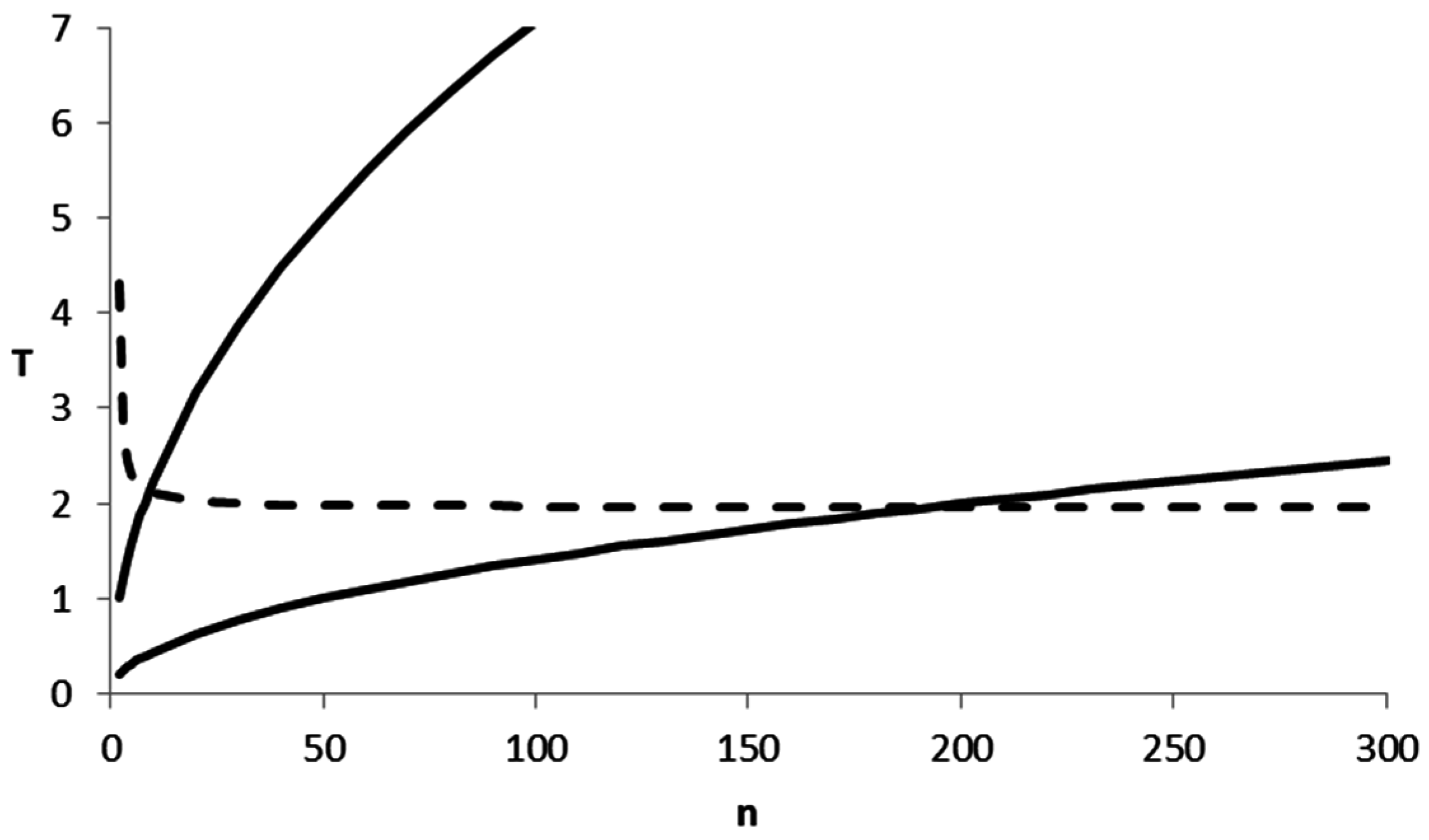
The NHST procedure has been criticized fiercely for quite a few decades; see for instance [16,17,18,19,20,21]. In the present study, we wish to single out one aspect: the test statistic $T$ scales with $\sqrt{n}$. A sample size $n=1000$ gives a $10$ times larger value of $T$ than a sample size $n=10$, and a sample size $n=100,000$ a $100$ times larger value, while keeping the effects and $\mathsf{\sigma }$ fixed. At a significance level $\mathsf{\alpha }=0.05$, the critical values of $T$ are $2.101$ ($n=10$; $\mathsf{\nu }=18$), $1.961$ ($n=1000$; $\mathsf{\nu }=1998$), and $1.960$ ($n=100,000$; $\mathsf{\nu }=199,998$), so if we simplify to $t_{crit,upper,0.05}\approx 2$, the only term that really matters is the observed value of the $T$ statistic. We reject $H_0$ when $\left|T\right|\ge t_{crit,upper,\mathsf{\alpha }}$, so when

$$\left|\frac{\overline{Y_B}-\overline{Y_A}}{S_P}\right|\gtrsim t_{crit,upper,\alpha }\sqrt{\frac{2}{n}}$$

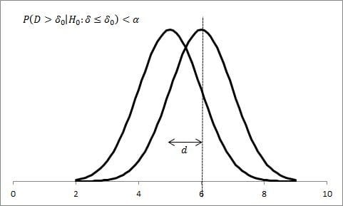
As an example, consider the case $\overline{Y_A}=5$, $\overline{Y_B}=6$, $S_P=1$, and let $n=2,\dots ,300.$ At $n\ge 9$, we have sufficient certainty to reject equality of means. When the difference is smaller, say $\overline{Y_B}=5.2$ instead, $n=9$ will not suffice; however, with a greater effort ($n\ge 194$), we will finally be able to reject equality of means (see Figure 1).

This convincingly reminds us that the decision to reject $H_0$ and to conclude that the two means are “significantly different” depends not only on the inherent properties of the populations (${\mathsf{\mu }}_A$, ${\mathsf{\mu }}_B$, $\mathsf{\sigma }$) or the properties of the samples that have been generated from them ($\overline{Y_A}$, $\overline{Y_B}$, $S_P$), but also on the sample size $n$, which is not an inherent property of the population. The concept of statistical significance mixes a number of aspects:

• the difference ${\mathsf{\mu }}_B-{\mathsf{\mu }}_A$ or its estimate, $\overline{Y_B}-\overline{Y_A}$;
• the standard deviation of the two populations, $\mathsf{\sigma }={\mathsf{\sigma }}_A={\mathsf{\sigma }}_B$, or its pooled estimate $S_P$;
• the sample size, $n$.

The first of these is natural: the actual difference between $\overline{Y_A}$ and $\overline{Y_B}$ is of course important in deciding if the difference is “large”, “substantial”, or—why not—“significant”.

The second one plays a more intricate role. The ratio $\frac{\overline{Y_B}-\overline{Y_A}}{S_P}$ provides a dimensionless indicator of the “relative” difference between the two means ${\mathsf{\mu }}_A$ and ${\mathsf{\mu }}_B$. It is sometimes described as a signal-to-noise ratio [16].

The third element plays a curious role. Sample size is important for establishing the confidence level of a result. However, sample size is not part of the nature of the phenomenon under investigation. The two means (${\mathsf{\mu }}_A$ and ${\mathsf{\mu }}_B$) and the standard deviation ($\mathsf{\sigma }$) are aspects of the research object. Sample size ($n$) is an aspect of the instrument that we use to probe the object. Of course, the quality of the instrument has an influence on the outcome. If we wish to know how many stars there are, and use a cheap telescope, the number will be lower than when we use a multi-billion dollar telescope. However, no serious astronomer will proclaim that the number of counted stars is equal to the number of starts in the universe. Instead, a formula to estimate the number of starts from the number of counted stars and the quality of the telescope will be developed. The application of this formula to the two measurement set-ups will give different results, and probably the estimate with the expensive telescope will be more accurate. In traditional NHST, this is different. What you see depends on the measurement set-up, and this is not corrected for in the outcome.

A consequence is that money can buy significance. Of course, the mean blood pressure of two groups of patients will never be equal when you consider the last digit. However, it may be that the difference is only in the fourth decimal, that $\overline{y_A}=120.0269$ and $\overline{y_B}=120.0268$. With an exceptionally large study, this negligible difference can be declared to be “significant”. The distinction between a significant difference and a large difference is mentioned in most textbooks on statistics, but often in a slightly cursory way, and it is well-known that many less-informed students and scientists mistake a significant difference for a large or important difference [22].

Combining the estimated difference $\overline{Y_B}-\overline{Y_A}$ and the standard error of this difference $S_P/\sqrt{n}$ into one formula $\frac{\overline{Y_B}-\overline{Y_A}}{S_P/\sqrt{n}}$ has one big advantage: it yields one single number, which can moreover objectively be tested against a conventional benchmark, such as $\mathsf{\alpha }=0.05$. Therefore, we only need to communicate this single number, either as a $t$-value, as a $p$-value, or as a significance statement, such as “$p<0.01$”, “**”, or “highly significant difference”. The fact that two things are combined in one is the root of the problem, however: information has been lost due to the compression of two complimentary aspects into one.

4. Alternatives to NHST for Comparing Two Means

Moving away from significance tests in the direction of effect sizes has been propagated by various authors [19,23], the latter of whom used the term “new statistics” to refer to this change of paradigm. Cumming [19] makes a strong plea for the use of confidence intervals. Confidence intervals for a difference of means, such as “95% CI $\left[1.4, 8.6\right]$” (p. 161) indeed display elements of size and significance, and use two pieces of information, not one.

Ziliak and McCloskey [16] popularize the two elements as “Oomph” and “Precision”. These two authors introduce more interesting expressions, such as “the sizeless scientist”, who only focusses on the question if there is an effect, and ignores if the effect is large or otherwise important. Such critiques on NHST are understandable, but it is questionable if the alternatives provide a real improvement.

A confidence interval shares a problem with the old statistics of NHST: given a large enough sample, the width of the confidence interval will shrink to zero, and as students are trained to see if the no-effect value of 0 is inside or outside the confidence interval, at some point the confidence interval approach will still be used more to assess the precision rather than the oomph. Of course, we could train students to ignore the question if 0 is inside the confidence interval, and to more focus on the confidence interval as such, but there are alternatives which in our view do a better job, and which are moreover easier to communicate.

Cumming [19] also advocates for effect sizes, where an effect size is “the amount of anything of research interest” (p. 162). In line with [23], we single out the standardized difference of means, often referred to as Cohen’s $d$, defined by

$$d=\frac{\overline{y_B}-\overline{y_A}}{s_P}$$

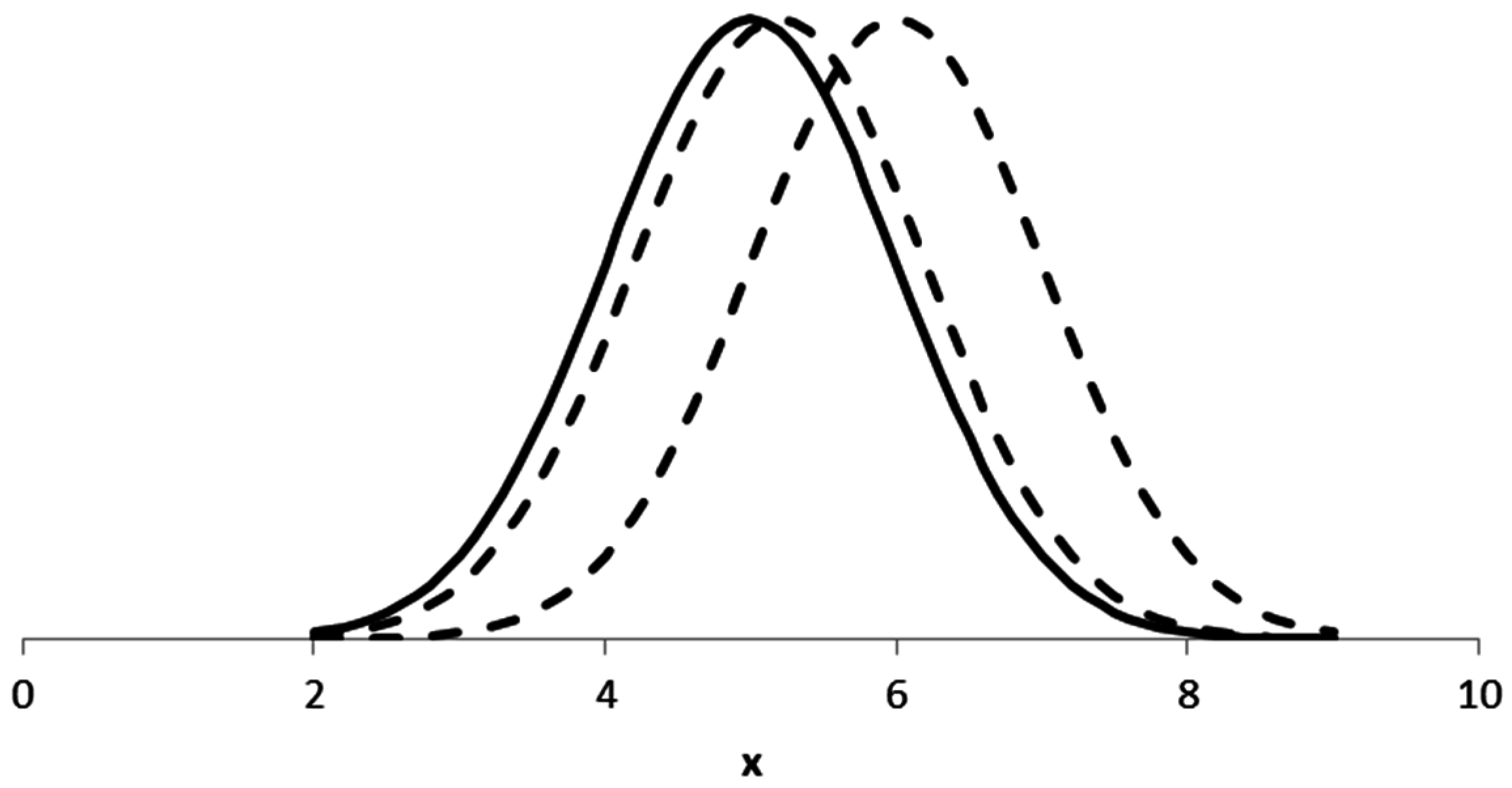
as a measure of effect size, because it basically expresses a signal-to-noise ratio. Cohen [23] arbitrarily proposed a categorization of values: $0.2$ means a small standardized effect size, $0.5$ a medium one, and $0.8$ is large. Figure 2 illustrates that even a more-than-large value of $d=1.0$ has a substantial overlap (around $45\%$) of probability mass. For $d=0.2$, the overlap is around $85\%$.

Finally, we mention the developments in non-inferiority trials tests, where a “margin”—denoted as $\mathsf{\Delta }$—is defined such that a proposed new drug can be tested to be not unacceptably worse than an existing one, while it may also be used for testing superiority [24,25]. A null hypothesis significance test then takes this margin into account. While developed in an environment of clinical research, where the existing drug is well studied, this approach has definite benefits. In a context of two alternatives (i.e., the sustainability of large scale fisheries and small scale fisheries), the situation is different, and there is no a priori magnitude for such a margin of non-inferiority or superiority. As such, we are looking for a margin of non-inferiority or superiority that is magnitude-independent. Such a measure is provided by the standardized effect size, here implemented as the standardized difference of means, discussed above. Although we agree with many points of critique on the standardized effect size in comparison to the “simple” effect size [26], we think they serve one important role in setting a generic standard for “oomph”, as introduced by Cohen [23]. Combining the idea of superiority with a margin [24,25] formulated in terms of the standardized effect size [23] is the core of our idea; see the next section.

5. A Proposal to Base Significance on Non-Trivial Effect Sizes

Under the null hypothesis, the standardized effect size is known to follow a non-central t-distribution [27]. However, it is seldom used, except for finding a confidence interval of the effect size. In fact, it has become fashionable to oppose effect sizes and significance tests [19]. We feel that embracing confidence intervals while abolishing significance tests is tantamount to throwing the baby out with the bathwater. Our aim is to reconcile significance tests (precision) with effect sizes (oomph). Below is a proposal to do so.

Our proposal is based on the following premise: an effect is “significant”

• when the effect size is large enough;
• and when it has been established with enough precision.

We now propose to operationalize this as follows:

• in advance, we set (as usual) a significance level $\mathsf{\alpha }$, say $\mathsf{\alpha }=0.05$;
• in advance, we set an importance level ${\mathsf{\delta }}_0$, say ${\mathsf{\delta }}_0=0.2$ (a small effect size);
• we define a test statistic $D=\frac{\overline{Y_B}-\overline{Y_A}}{S_P}$ that estimates $\mathsf{\delta }=\frac{{\mathsf{\mu }}_B-{\mathsf{\mu }}_A}{\mathsf{\sigma }}$;
• we test the null hypothesis $H_0:\mathsf{\delta }\le {\mathsf{\delta }}_0$ at a significance level $\mathsf{\alpha }$.

In this way, we ensure that a rejected null hypothesis means both a “substantial” effect size and sufficient precision. A p-value larger than $\alpha$ means that the observed signal-to-noise ratio $d$ is too small to disprove the null hypothesis, which occurs with a small effect no matter the size of the sample, or with a small sample no matter the size of the effect. A sufficiently large effect size measured with sufficient precision will reject the null hypothesis.

Under the least extreme version of the null hypothesis, ($\mathsf{\delta }={\mathsf{\delta }}_0$), the distribution of the test statistic $D$ is as follows:

$$T =\frac{\left(\overline{Y_B}-\overline{Y_A}\right)-\left({\mathsf{\mu }}_B-{\mathsf{\mu }}_A\right)}{S_P\sqrt{\frac{2}{n}}}=\frac{D-{\mathsf{\delta }}_0}{\sqrt{\frac{2}{n}}}~t\left(\mathsf{\nu }=2\left(n-1\right)\right)$$

It is important to observe that the p-value obtained from this t-test (let us call it $p_2$, for a two-sided test $\mathsf{\delta }={\mathsf{\delta }}_0$) is not the p-value of the question ($p_1$, for a one-sided test $\mathsf{\delta }\le {\mathsf{\delta }}_0$), but must be further processed according to the following scheme:

$$p_1=\{\begin{array}{cc}\frac{1}{2}{p}_2& \mathrm{if}d<{\mathsf{\delta }}_0\\ 1-\frac{1}{2}{p}_2& \mathrm{if}d>{\mathsf{\delta }}_0\end{array}$$

where $d$ is the obtained value of the $D$-statistic.

As an illustration, we reconsider the earlier example, $Y_A~N\left(5,1\right)$ and $Y_B~N\left({\mathsf{\mu }}_B,1\right)$ with two choices for ${\mathsf{\mu }}_B$: $5.2$ and $6.0$. Samples are generated with $n=1000$. The results are presented in

Table 1. Simulation results with sample size $n=1000$ and population effect size $\mathsf{\delta }=0.2$ (second column) and $\mathsf{\delta }=1.0$ (third column).

Parameter/Statistic	Small Effect Size	Very Large Size
${\mathsf{\mu }}_2$	$5.2$	$6.0$
$\mathsf{\delta }$	$0.2$	$1.0$
$d$	$0.243$	$0.969$
$t$	$0.927$	$17.310$
$p_2$	$0.354$	$0.000$
$p_1$	$0.823$	$0.000$
reject $H_0:\mathsf{\delta }\le 0.2$ at $\mathsf{\alpha }=0.05$?	no	yes

.

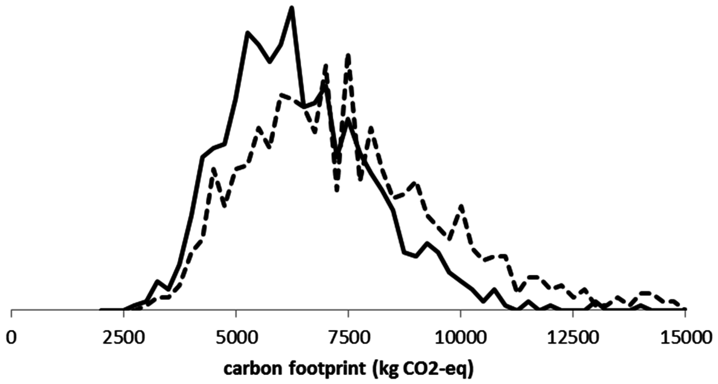
We conclude with a real case illustration for the fisheries [9]. Monte Carlo simulations of the carbon footprint for small-scale and large-scale fisheries with $n=1000$ yielded the results of

Table 2. Monte Carlo simulation results of the carbon footprint of small fisheries and large fisheries, using sample size $n=1000$.

Statistic	Value
$d$	$0.489$
$t$	$9.153$
$p_2$	$0.000$
$p_1$	$0.000$
reject $H_0:\mathsf{\delta }\le 0.2$ at $\mathsf{\alpha }=0.05$	yes

. Figure 3 shows the values in a histogram.

As an aside, the assumptions of the performed test are not fully justified in this illustration. Variances are unequal, so the Welch form of the test would have been more appropriate. However, our aim is to illustrate the idea, and in our experience, the Welch form in most cases yields similar results.

6. Discussion

We believe that our proposal resolves a dilemma in the application of statistical techniques to large datasets. Traditional significance tests focus on precision and ignore size, while the “new statistics” [19] emphasize size and include precision only indirectly. The proposed solution of defining the tuple $\left(\mathsf{\alpha },{\mathsf{\delta }}_0\right)=\left(0.05, 0.2\right)$ at the outset and then testing $H_0:\mathsf{\delta }\le {\mathsf{\delta }}_0$ combines precision and size. Like the old statistics, it still provides an unambiguous statement in the form “there is a significant difference between the two populations”, which now combines statistical evidence with empirical relevance.

One may object that our new procedure for the assessment of a significant difference of means involves an arbitrary element—namely, choosing ${\mathsf{\delta }}_0$. That is true, but the choice of $\mathsf{\alpha }$ is subjective as well, and yet it is part of the mainstream “objective” NHST procedure. Of course, depending on the context, different choices of the tuple $\left(\mathsf{\alpha },{\mathsf{\delta }}_0\right)$ may be made.

Another possible objection is the lack of novelty. In fact, we believe that it is precisely the lack of revolutionary features that is a strong point of our proposal. Mainstream NHST is highly institutionalized, through at least two generations of textbooks, through statistical software (Excel, SPSS, SAS, etc.) and through guidelines for reporting in the social and behavioral sciences (primarily APA). While many writers have published pleas to abolish NHST, progress has been limited so far (APA now recommends the reporting of effect sizes). Our proposal falls within NHST, with a central role for an a priori null hypothesis and $\mathsf{\alpha }$. The only change is that the usual and often implicit null hypothesis of “no difference” (${\mathsf{\mu }}_A={\mathsf{\mu }}_B$) be replaced by a more interesting null hypothesis of “at least small difference” (e.g., $\frac{{\mathsf{\mu }}_B-{\mathsf{\mu }}_A}{\mathsf{\sigma }}\le 0.2$). This is emphatically not a Neyman–Pearsonian direction, because the null hypothesis is still composite (e.g., $\frac{{\mathsf{\mu }}_B-{\mathsf{\mu }}_A}{\mathsf{\sigma }}>0.2$), and because the procedure allows for $p$-values as well as significance statements. Our proposal to some extent resembles earlier ones made in the context of Bayesian statistics [28]. Again, despite the methodological attractiveness of the Bayesian framework, just the fact that the mainstream is not Bayesian is, from a strategic point of view, a sufficient argument for proposing modifications to the classical framework. On the longer term, however, Bayesian approaches may solve some of the issues in a more fundamental way, employing the Bayesian information criterion [14,29], using the Bayes factor [30], or probability–possibility transformations [31,32,33]. Schumi and Wittes [24] also briefly discuss the classical approach in a way that is quite similar to ours, although formulated in terms of a one-sample hypothesis. It is primarily from the comparative set-up that our proposal derives its appeal: a difference between two treatments must be sufficiently significant and sufficiently large. Our proposal also shares elements with [34], which connects it to power calculations. Again, as power is formally part of NHST, it is rarely practiced by researchers in the applied sciences. Our testing scheme involving the tuple $\left(\mathsf{\alpha },{\mathsf{\delta }}_0\right)$ has a strategic value in staying close to existing practice, while attempting to remediate the most pressing problem.

Although the issue mentioned (namely: “what do we mean by a significant difference?”) is not a problem that exclusively occurs in the world of computer simulations, meta-analysis, and big data, we think that the developments since the start of the 21st century require a renewed confrontation with the criticism on NHST. We even think that a solution must be provided: an easy solution, close to the established practice. Our proposal is one step in a longer series of steps.

The described procedure was restricted to the case that ${\mathsf{\mu }}_A$ is smaller than ${\mathsf{\mu }}_B$. This can be easily generalized to the opposite case. More importantly, it can also be generalized to the two-sided case, in which the null hypothesis $\left|\frac{{\mathsf{\mu }}_B-{\mathsf{\mu }}_A}{\mathsf{\sigma }}\right|\le {\mathsf{\delta }}_0$ is tested. A rejection of this hypothesis implies that we conclude that the absolute value of the standardized effect size $\left|\mathsf{\delta }\right|$ is larger than ${\mathsf{\delta }}_0$.

Another generalization is that of comparing more than two populations. A typical approach is the ANOVA form, in which the null hypothesis is ${\mathsf{\mu }}_A={\mathsf{\mu }}_B={\mathsf{\mu }}_C$, etc. This is less trivial to generalize for the $\left(\mathsf{\alpha },{\mathsf{\delta }}_0\right)$ procedure. The alternative of making several pairwise comparisons, each with a Bonferroni-corrected $\left(\mathsf{\alpha }\text{′},{\mathsf{\delta }}_0\right)$ where $\mathsf{\alpha }\text{′}<\mathsf{\alpha }$ seems a natural way to go.

A third generalization is the direction of heteroskedastic populations, where ${\mathsf{\sigma }}_A\ne {\mathsf{\sigma }}_B$.

There is potential to further generalize the proposed procedure for statistics other than the standardized effect size (such as correlation coefficients, regression coefficients, and odds ratios), for cases with dependent distributions (using the paired t-test), and for cases in which the populations are not normal (requiring the Mann–Whitney test or another non-parametric method).

The era of almost unlimited computer capacity has created studies with tremendous pseudo-samples using Monte Carlo simulation, bootstrapping, and other methods. In addition, the internet has created almost unlimited data repositories, which also result in huge samples. This has eradicated many of the fundamental assumptions of traditional inferential statistics, which have been developed for small samples. Willam Gosset (“Student”, [35]) developed his t-distribution to assess small samples, even as small as $n=2$ [10]. Bootstrapping has been at the center of this development, with formulas even suggested for setting a sample size to satisfy significant differences [36,37]. However, even traditional statistical textbooks typically devote a few pages to choosing sample size such that a significant result will be obtained (e.g., [1,2,3]). The fact that this significance refers to a basically meaningless (“sizeless”) phenomenon is hardly mentioned. This is clearly a questionable practice that easily leads to the justified rejection of meaningless null hypotheses, which is exactly the problem raised by those who criticize NHST, such as Ziliak and McCloskey [16]. However, precision is important, and that is what the alternative schemes [19] have been underemphasizing. Data analysis in the era of large samples requires a new paradigm. Our proposed reconciliation of effect size and precision (by setting the tuple $\left(\mathsf{\alpha },{\mathsf{\delta }}_0\right)$ in advance) should be seen as one seminal step in this program. Whereas we have not applied its working to meta-analysis and big data, and have only demonstrated its application to computer-generated samples of size $1000$, we believe that the problem is serious enough to deserve more attention in the era of increasing sample sizes.

As indicated, Bayesian concepts might further alleviate some of the problems mentioned, as might a return to the Neyman–Pearson framework. However, our proposal is an attempt to improve the situation with a minimum of changes, only replacing one conventional choice ($\mathsf{\alpha }$) by a tuple of conventional choices ($\mathsf{\alpha },{\mathsf{\delta }}_0$). Piecemeal change may be a better solution than revolution in some cases.