Article

Field Scale Assessment of the TsHARP Technique for Thermal Sharpening of MODIS Satellite Images Using VENµS and Sentinel-2-Derived NDVI

1
Department of Crop and Soil Sciences, University of Georgia, Tifton, GA 31793, USA
2
Institute of Agricultural Engineering, Agricultural Research Organization (ARO), Volcani Center, Rishon Leziyyon 7505101, Israel
3
The Blaustein Institutes for Desert Research, Ben-Gurion University of the Negev, Sede Boqer Campus, Midreshet, Ben-Gurion 84990, Israel
4
Department of Agronomy and Agrotechnology, University of Thessaly, 41500 Larissa, Greece
*
Author to whom correspondence should be addressed.
Remote Sens. 2021, 13(6), 1155; https://doi.org/10.3390/rs13061155
Submission received: 28 December 2020 / Revised: 12 March 2021 / Accepted: 14 March 2021 / Published: 18 March 2021

Abstract

:
Remotely sensed-based surface temperature is an important tool for crop monitoring and has great potential for improving irrigation management. However, current thermal satellite platforms do not display the fine spatial resolution required for identifying crop water status patterns at the field scale. The thermal sharpening (TsHARP) utility provides a technique for downscaling coarse thermal images to match the finer resolution of images acquired in the visible and near infrared bandwidths. This sharpening method is based on the inverse linear relationship between vegetation fraction calculated from the normalized difference vegetation index (NDVI) and land surface temperature (LST). The current study used the TsHARP method to sharpen low-resolution thermal data from the Moderate Resolution Imaging Spectrometer MODIS (1 km) to the finer resolution of Sentinel-2 (10 m) and Vegetation and Environment New micro-Spacecraft (VENµS) (5 m) visible-near infrared images. The sharpening methodology was evaluated at scene and field scales in southern Georgia and northern Mississippi, USA. A comparison of sharpened temperature was made with reference temperatures from Landsat-8 Operational Land Imager (OLI) in four different spatial resolutions (30, 60, 120, and 240 m) for method validation. Coarse resolution comparison on the dates in which imagery from both sensors were acquired on the same day resulted in average observed mean absolute error (MAE) of 1.63 °C, and R2 variation from 0.34 to 0.74. Temperature errors at the field scale ranged from 0.25 to 3.11 °C using both Sentinel-2 and VENµS. Sharpened maps at 120 and 60 m resolution showed the highest consistency for all fields and dates. Maps sharpened using VENµS images showed comparable or higher accuracy than maps sharpened using Sentinel-2. The superior performance coupled with the better revisit time indicates that the VENµS platform has high potential for frequent in-season crop monitoring. Further research with ground data collection is needed to explore field use limitations of this methodology, but these results give useful insights of potential benefits of implementing the TsHARP technique as a tool for crop stress monitoring.

1. Introduction

Thermal remote sensing uses thermal infrared (TIR) bands in the 8 to 14 µm region of the electromagnetic spectrum in which atmospheric absorption effects are attenuated [1]. At the molecular level, plant absorption in the TIR bands is influenced by the absorption properties of leaf tissues driven by molecular vibration [2]. At the physiological level, absorption is directly influenced by the transpiration rate [3]. In drought conditions, plants that exhibit isohydric behavior tend to close their stomata to maintain leaf water potential (LWP). This decreases their transpiration rate significantly, leading to an increase in leaf temperature [4]. The direct relationship between changes in leaf temperature resulting from changes in LWP makes TIR bands more sensitive to detecting water stress than other regions of the electromagnetic spectrum. Because of this, thermal imagery has become increasingly important in monitoring of water status for irrigation management [5] in crops such as coffee [6], cereals [7,8], and soybean and cotton [9].
Thermal infrared temperature maps can be used to estimate LWP and create LWP maps at the field scale. In turn, the LWP maps may be used to delineate LWP-based irrigation management zones (IMZs) for site-specific irrigation [10]. The spatial resolution of currently available satellite-based thermal imagery is not fine enough to identify crop water status patterns at the field scale. Satellite platforms such as Terra MODIS (Moderate Resolution Imaging Spectroradiometer) and NOAA-AVHRR (National Oceanic and Atmospheric Administration–Advanced Very High-Resolution Radiometer) have a very high temporal resolution (1 day), but a coarse spatial resolution of 1 km [11]. Conversely, Landsat Thematic Mapper—TM, Landsat Enhanced Thematic Mapper Plus—ETM+, and Landsat Operational Land Imager—OLI, have higher spatial resolution of 120, 60, and 100 m respectively, but a low revisit time of 16 days. While Landsat datasets have a finer resolution, its low temporal resolution is not adequate for frequent monitoring required during the growing season for irrigation decisions. The occurrence of clouds can further decrease the availability of usable images.
To address this tradeoff problem between low-resolution images with high revisit time and high-resolution images with low revisit time, sharpening methodologies to downscale TIR coarse resolution have been proposed [12]. These techniques to disaggregate land surface temperature (LST) are found in the literature under a variety of terms, such as thermal sharpening, subpixel temperature estimation, downscaling LST, component temperature retrieval, spatial enhancement of LST, and others [13], but they can be classified into two main categories, called temperature unmixing and thermal sharpening. The main difference between these two groups is that in temperature unmixing, the goal is to decompose the coarse mixed pixel temperature into its existing elements through temporal, spatial, and spectral observations, while thermal sharpening aims to enhance the thermal image by exploring the correlation between LST and auxiliary data such as vegetation cover [14].
Thermal sharpening is the category most frequently used for downscaling thermal images. One of the earliest works using spatial sharpening dates back to 1985, wherein Landsat-4 Thematic Mapper (TM) thermal imagery was sharpened to 30 m resolution using a multiband least squares method [15]. This approach was possible due to the high correlation between the TM bands in agricultural scenes. A thermal image estimate was created using a coefficient predicted from Landsat-4 TM visible and infrared bands that was then used to enhance the spatial resolution on the original thermal band.
Over the last 30 years, a variety of new sharpening algorithms have been suggested including the thermal sharpening (TsHARP) technique that was improved from the Disaggregation procedure for radiometric surface temperature (DisTrad) algorithm developed by Kustas et al. [16]. The DisTrad method uses the relationship between radiometric surface temperature and the Normalized Difference Vegetation Index (NDVI) to disaggregate temperature data at the NDVI finer image resolution. The NDVI resolution is first aggregated to the coarser resolution of the brightness temperature (BT) image and a second degree polynomial least-squares regression is fitted between the two variables. In this study, airborne images were used to estimate temperatures over the southern Great Plains by sharpening MODIS images to 200 m and provided temperature errors of ~1.5 °C. Agam et al. [11] proposed an improvement from the DisTrad algorithm by using vegetation fraction as the dependent variable instead of NDVI. Different types of land cover in a scene can cause increased number of outliers in the two ends of NDVI values.
A summary study published in 2013 [13] indicated that Landsat TM and Terra Advanced Spaceborne Thermal Emission and Reflection Radiometer (ASTER) were the satellite platforms most frequently used for LST disaggregation. At the time, MODIS was a much younger platform, and since then has become widely utilized in downscaling approaches due to the high temporal frequency in which images are made available. With MODIS images collected on a daily basis, the availability of datasets for sharpening during the growing season depends on the satellite platforms used to derive visual and NIR (VNIR) data. Landsat 7 ETM+ [14,17] and Landsat-8 OLI [18] are commonly used to build the LST-NDVI regression and can generate roughly two sharpened images. Sentinel-2 has a higher revisit time and offers the potential of more sharpened images during the season. Clouds may greatly reduce the availability of useable images, especially in areas with frequent cloud cover.
Sentinel-2 is a two-satellite platform operated by the European Space Agency (ESA) as part of the Copernicus earth observation program which became operational [19] in 2015. The two satellites are in the same orbit but spaced 180° apart. They provide data in 13 different spectral bands (443–2190 nm) with spatial resolutions of 10, 30, and 60 m and a revisit time of 5 days. Sanchez et al. [20] used Sentinel-2 VNIR data to sharpen MODIS images to a 10 m resolution over experimental fields in southeastern Spain. Over a period of 2 months, they sharpened LST images on 6 different days.
In 2017, a super-spectral micro-satellite resulting from a partnership between the Israel Space Agency (ISA) and the French National Centre for Space Studies (CNES) was launched [21,22]. The Vegetation and Environment New micro-Spacecraft (VENµS) was intended to increase land data acquisition to, among other purposes, improve modeling of vegetation processes. This minisatellite has a revisit time of 2 days, a spatial resolution of 5.3 m, and a spectral resolution of 12 bands (420–910 nm). Although the unique features of this low-orbit satellite show great potential for increased dataset frequency, to our knowledge, no studies have explored the use of VENµS in thermal sharpening methodologies.
The majority of sharpening studies cited above explored the use of sharpening for large scene scales. However, very few studies have been conducted exploring the feasibility of using this technique in crop fields to aid in management decisions. In this context, the main goal of this work was to assess the use of the TsHARP technique to sharpen MODIS images using Sentinel-2 and VENµS in the southeastern USA at field scale and to assess if sharpened images have the potential to be used at the field scale for delineating irrigation management zones (IMZs) for variable rate irrigation in cotton. Applying this technique to this region is especially challenging because of frequent cloud cover during the growing season. The TsHARP use at scene scale was also assessed. Specific objectives were to compare the performance of the TsHARP technique using data from the two satellite platforms on overlapping dates.

2. Materials and Methods
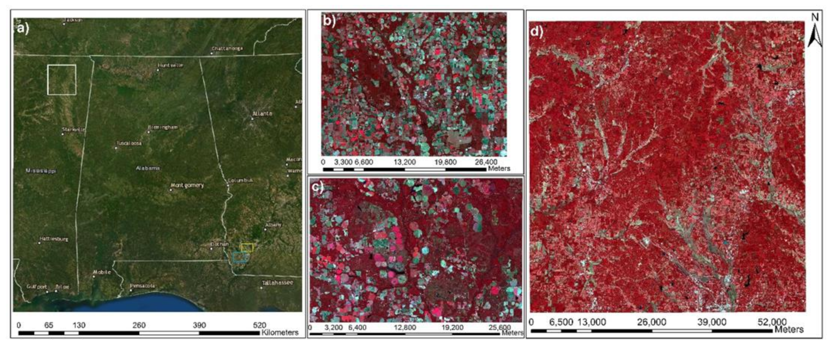
2.1. Study Sites

This study was conducted in three different locations of the southeastern USA in which cotton is an important crop (Figure 1) using imagery from the 2019 growing season. The first and second study sites are located in southwestern Georgia and centered around 84°44′28″W, 31°11′28″N, and 84°33′7″W, 31°26′42″N. The third study site is located in northeastern Mississippi centered around 88°51′42″W, 34°31′58″N. The Miller County scene (hereafter referred as to scene 1) is mostly composed of cotton fields, followed by woody wetlands, pine forest, and peanut fields. Land cover in scene 2, located in Baker County, Georgia, was 40% woody wetlands followed by pine forest, and cotton and peanut fields. The land cover in scene 3, located around Union County, Mississippi, was composed mostly of various types of forest, followed by pasture and soybean fields. All locations have similar subtropical climates with high humidity and hot summers, with the average air temperature of the hottest month (July) being equal to or greater than 22 °C [23,24]. The minimum and maximum average temperatures from July to November in the last 20 years were 15.6 and 27.4 °C [25].
The United States Department of Agriculture (USDA) National Agricultural Statistics Service’s (NASS) Cropland Data Layer (CDL) hosted by CropScape (https://nassgeodata.gmu.edu/CropScape/ (accessed on 9 July 2020)) was used to identify fields that were planted with cotton during the 2019 growing season. Extensive agricultural ground truth data acquired from the Common Land Unit (CLU) data from the USDA Farm Services Agency (FSA) is coupled with moderate resolution satellite images to create yearly crop-specific land cover maps of the whole continental United States [26]. A total of 22 cotton fields were identified for this study, with field sizes ranging from 14 to 164 ha (Table A1).

2.2. Satellite Images Acquisition and Processing

Thermal images from MODIS and Landsat-8 Operational Land Imager (OLI) were acquired in all three locations on dates within the cotton growing period ranging from August to November 2019 (Table 1). The MODIS product used was MODIS/Thermal Bands Daily L2B-Lite Global (MODTBGA), and it was download from the National Aeronautics and Space Administration (NASA) Earth Data Search website (https://search.earthdata.nasa.gov/search (accessed on 15 April 2020)). MODTBGA version 6 is available daily with a spatial resolution of 1 km (km) with sinusoidal projection, and it consists of brightness temperature data from three MODIS bands (bands 20, 31, and 32) [27]. After download, MODIS images were pre-processed using ArcGIS (Esri, Redlands, CA, USA). In ArcMap version 10.2.2 (Esri, Redlands, CA, USA), MODIS band 31 was re-projected to the World Geodetic System (WGS) 1984 zone 16, and a scale factor of 0.01 was used to obtain brightness temperature values. Landsat-8 OLI images were downloaded directly from the United States Geological Survey (USGS) Earth Explorer website (https://earthexplorer.usgs.gov/ (accessed on 20 April 2020)). Landsat-8 provides images with 15 (panchromatic), 30, and 100 m (thermal) spatial resolution. However, thermal bands are disaggregated to 30 m resolution images by the Landsat Science team and are made publicly available. Landsat-8 pre-processing was performed by using the Semi-Automatic Classification Plugin (SCP) in QGIS 3.14.0 (QGIS Development Team, 2020) [28]. SCP offers pre-processing and post-processing tools for a variety of satellite images [29]. Radiometric calibration was performed on Landsat-8 thermal infrared band 10 (10.6–11.19 μm), where the DOS1 (Dark Object Subtraction) atmospheric correction technique was used to convert data to Top of Atmosphere (TOA), and correct for solar irradiance effects. SCP was also used to convert values to brightness temperature in Celsius.
Visual-near infrared (VNIR) data from Sentinel-2 was used for sharpening in all three locations. Images were downloaded from the USGS Earth Explorer website. SCP was used to perform atmospheric correction in all Sentinel-2A images. The SCP used DOS1 atmospheric correction for Sentinel-2 images as well. Band 8 (842 nm) and band 4 (665 nm) were used to calculate NDVI. VNIR images from VENµS were also utilized for thermal sharpening of MODIS. VENµS data were only available for the scenes in Georgia (Miller and Baker counties). Images were download from the Theia Data and Services Center for continental surfaces (https://www.theia-land.fr/en/data-and-services-for-the-land/ (accessed on 20 April 2020)). VENµS-based NDVI was calculated using bands 11 (865 nm) and 5 (620 nm) from the level 2 product. VENµS level 2 product provides fine cloud and shadow mask, and it is already atmospherically corrected.
Due to the differences in satellite temporal resolution, and frequent cloud coverage during the summer in the study areas, the difference in acquisition date among the satellites used for TsHARP implementation (MODIS, Sentinel-2, and VENµS) was up to one day and up to five days for validation (MODIS and Landsat-8).

2.3. TsHARP Methodology

As described previously, the TsHARP technique is based on the inverse relationship between LST and vegetation cover. The fractional vegetation cover (fc) is estimated from NDVI using Equation (1) [30]:
f c = 1 NDVI max NDVI NDVI max NDVI min 0.625
where NDVImax and NDVImin are the maximum and minimum NDVI values in the scene and NDVI is the index value in an individual pixel.
The fc image is aggregated to a coarser resolution to match with the coarse resolution of the LST image, and an empirical linear regression model is fitted, as shown by Equation (2):
L S T c o a r s e = a + b f c c o a r s e
where a and b are the intercept and slope resulting from the linear regression between LST and fc at coarse resolution.
Coefficients a and b are then applied to the fine-resolution fc data (fc fine) and fine-resolution NDVI to predict LST at a finer resolution (Equation (3)) [19]. Coefficients a and b are also applied to the fc image at coarse resolution to derive a new LST image. The difference between the original LST image and the newly derived image is used to calculate the residual error image at coarse resolution. The residual error image is then disaggregated to a fine resolution and applied to the LST at finer resolution to increase the prediction accuracy (Equation (4)). A detailed explanation of the TsHARP algorithm was provided by Agam et al. [11].
L S T f i n e = a + b f c f i n e
L S T p r e d i c t e d = L S T f i n e + r e s i d u a l   e r r o r

2.4. TsHARP Validation and Assessment

The complete workflow of the TsHARP technique can be divided into two steps (Figure 2. Flowchart of the thermal sharpening (TsHARP) methodology, including inputs, outputs, and processing steps, and methodology validation using Landsat-8 images (modified after Huryna et al. [19]). The first step is the sharpening of MODIS images using Sentinel-2- and VENµS-derived NDVI to finer resolutions. The second step is the validation of the method by comparing the sharpened temperature with a reference temperature from Landsat-8 images at 30, 60, 120, and 240 m spatial resolution. The TsHARP validation was performed by fitting a linear regression model to MODIS BT and Landsat-8 BT images in the coarse and finer resolutions. The validation was performed at the scene scale for all dates for which images were downloaded and for selected dates at the field scale (See Table 1).
The methodology performance assessment was estimated using different quantitative statistics approaches [31]. Coefficient of determination (R2), root mean square error (RMSE), mean absolute error (MAE), and bias (Equations (5)–(8)) were calculated to estimate the level of agreement between predicted and reference temperatures:
R 2 = 1 T s h a r p T r e f   2 T s h a r p T r e f _ m e a n   2
R M S E =   n 1 i = 1 n T s h a r p T r e f 2 1 / 2
M A E =   n 1 i = 1 n T s h a r p T r e f
b i a s =   i n 1 T s h a r p T r e f n

3. Results and Discussion

3.1. Scene Scale

The thermal sharpening validation was performed for a total of 14 dates using the MODIS/Sentinel-2 and MODIS/VENµS BT-NDVI regressions (Table 1).

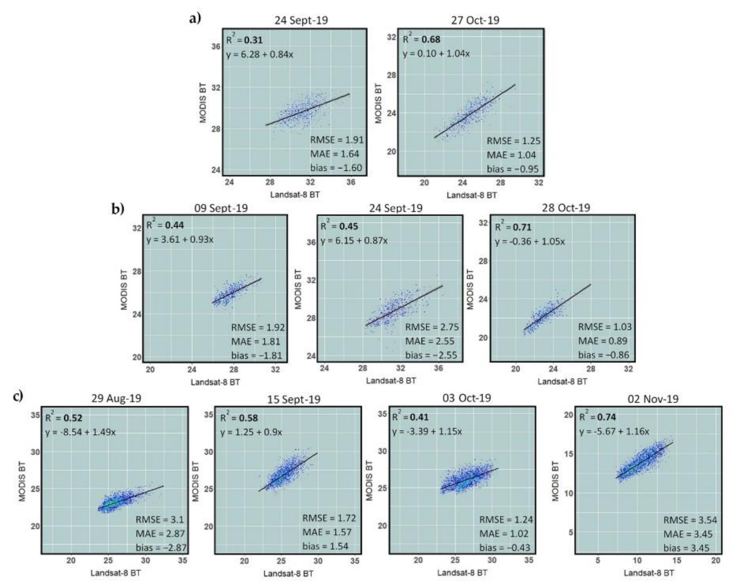
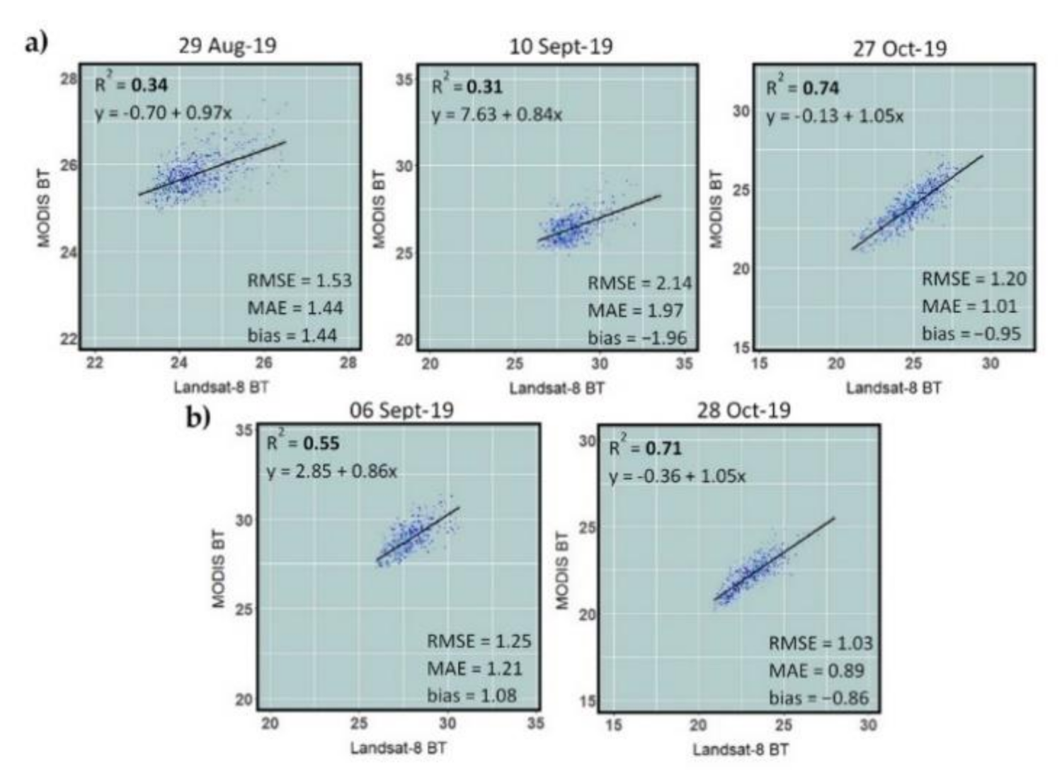
3.1.1. Sensors’ Comparison at Coarse Resolution

The correlations between MODIS brightness temperature (BT) and aggregated Landsat-8 BT at coarse resolution are shown in Figure 3. Results showed that the correlations between the BT of the two sensors were similar towards the end of the season (end of October and beginning of November) when average temperatures were in the low 20 °C or below, with coefficients of determination (R2) ranging from 0.68 in scene 1 to 0.74 in scene 3. The regression model coefficients, however, were different. Despite having the highest R2 among the three scenes, the sensor comparison of scene 3 presented the highest RMS error and positive bias of 3.54 °C. In scenes 1 and 2, the RMS errors in this period were below 1.25 °C, with a negative bias lower than 0.95.
In the months of August and September, correlations were overall lower, and varied with location. The lowest R2 values were observed in scene 1 (0.31) followed by the third date in scene 3 (0.41) and first date in scene 2 (0.44). The low relationship in these three dates can be attributed to cloud coverage in one or more images. Parts of the respective scenes were cropped to exclude areas affected by the clouds, substantially decreasing the number of pixels. In addition, methods utilized to mask clouds were not effective in removing areas under the clouds’ shadow. The combination of reduced number of pixels and BT values affected by cloud shadow led to a weaker relationship between sensor responses.
A negative bias was observed in 7 out of 9 dates and indicates that temperatures extracted from MODIS scene were cooler when compared to Landsat-8. The comparison between these two sensors yielded RMS errors no higher than 1.92 °C in 6 out of 9 dates. In the second date of scene 2, and the first and last dates in scene 3, the RMSE values observed were higher, with errors ranging from 2.75 to 3.45 °C. In 2 out of these 3 dates, the bias was positive and not negative like in most of the dates. No clear factors were found that can explain these deviations.
Similar results were observed in the selected dates for VENµS analysis (Figure 4). As mentioned earlier, VENµS images were only available for the two scenes in Georgia. The relationship between MODIS BT and Landsat BT was strong at the end of October when temperatures were lower, and weaker in the months of August and September. In the remaining dates, R2 values in scene 2 were again stronger than the ones observed in scene 1. The RMS errors varied between 1.03 to 2.14 °C in both locations. Similar to MODIS/Sentinel-2 sharpening, a negative bias was observed for 3 out of 5 dates, while a positive bias was obtained for the other 2 dates.
A study conducted in 2014 [32] reported differences between MODIS and Landsat satellite LST spatial distribution. Maximum temperatures showed a difference of about 15 °C. The range between minimum and maximum temperatures from Landsat were always wider than observed in MODIS (Table 2). In the study described here, towards the end of October, most of the crops were already harvested and fields had exposed soil, causing a more evident BT difference between dense vegetation and exposed soil, which could be more easily detected by the coarse spatial resolution from MODIS. During the months of August, September, and mid-October, most fields in the scenes still had vegetation cover from the crops, thus temperature changes were more subtle across different land covers. These subtle changes were depicted in the finer resolution from Landsat, leading to a wider range of temperature values compared to the smaller range from MODIS, resulting in a lower R2.
Coarse resolution sensor comparison showed that the BT range values of Landsat were always wider than observed in MODIS (Table 2). At one date (8/29), the Landsat BT range was double the MODIS BT and the max difference was as high as 6.4 °C. Similar results were observed by Weng et al. [32] when comparing Landsat TM LST to MODIS. In the two dates used in their study, similarities were observed only between minimum surface temperatures. Landsat TM maximum temperatures were considerably higher than in MODIS, causing great discrepancies in LST spatial patterns. Essa et al. [33] stated that surface temperature from MODIS were substantially lower than Landsat 7 ETM+ temperatures. A 5 °C mean temperature difference between the two sensors was achieved on six occasions. The results from 10 out of 14 dates examined in this paper showed a similar trend, where a negative bias was found between the two sensors. This consistently lower temperature presented by MODIS when comparing with Landsat sensors can be described as a systematic bias. Yet, the fact that some occasions showed different trends casts a shadow over this determination. The concept of systematic bias was discussed by Liu et al. [34]. A consistent bias between two satellites could be introduced by sensor measurement errors such as random noise. Satellite sensor-specific characteristics such as bandwidth, acquisition time, and orbit parameters are further causes of bias [32].

3.1.2. TsHARP Validation

Landsat-8 thermal images were aggregated to 60, 120, and 240 m to perform validation at the four spatial resolutions proposed, including Landsat’s original resolution of 30 m. Table 3 and Table 4 show the statistics of sharpened images compared to reference maps in all the scenes studied using both VENµS- and Sentinel-2-based NDVI, respectively. Validation of thermal sharpening resulted in an overall higher R2 than only comparing sensor brightness temperatures at coarse resolution. Sharpened accuracy was higher in coarser resolutions (120 and 240 m) in 10 of the 14 dates analyzed. In most remaining dates in which accuracy at 240 m was slightly lower than finer resolutions, portions of the scene had to be excluded prior to the analysis due to cloud cover. The decrease in the number of pixels in the 240 m resolution could have affected the sharpening accuracy. Based on the results, sharpening efficiency tended to decrease with increased targeted resolution. These findings are corroborated by results observed by Huryna et al. [19]. In their study, Landsat-8 and Sentinel-3 thermal imagery were resampled and then sharpened to 240, 120, and 60 m resolutions using Landsat-8 and Sentinel-2, respectively. In both cases, R2 values decreased and temperature uncertainty values increased as resolution increased, with highest error values of 1.17 and 1.45 °C for Landsat and Sentinel-3, respectively.
The coefficient of determination for Sentinel-2 validation dates in scene 1 ranged from 0.55 at 30 m resolution to 0.76 at 240 m, with highest values occurring on 28 October, while for VENµS dates, the lowest value was 0.48 at 30 m, and the highest value was 0.8 at 240 m (Table 4). In scene 2, the method’s accuracy in dates available tended to be higher than achieved in scene 1 for both Sentinel-2 and VENµS dates, with only three R2 values below 0.6. Remaining values for Sentinel-2 varied from 0.6 to 0.8 and for VENµS, from 0.63 to 0.79. In this scene (scene 1), the three weakest relationships were observed at the finer resolutions of 30 and 60 m. Scene 3 displayed a similar performance as the two previous scenes, with values ranging from 0.50 to 0.77, except on 3 October, wherein the Landsat-8 image had large areas in the middle of the scene covered by clouds and cloud shadow that were difficult to remove. The remaining affected pixels that were not excluded by the masking process affected the accuracy of validation. A 3 days difference in acquisition time between sharpened and reference images was observed and could have also been a cause of higher error, although no trend between error magnitude and time lag between satellites was observed.
Validation of sharpened maps had slightly higher RMS errors than the sensors’ BT comparison at coarse resolution, with uncertainty increasing as the aimed resolution became finer. The highest errors were observed in the first and third dates of scene 3, with error values around 3.04 and 3.78 °C. It is worth emphasizing that MODIS and Landsat had a 1-day difference in acquisition time when the highest error of almost 4 °C was observed. Lowest overall errors were observed in the last date of scene 2 for both Sentinel-2 and VENµS selected dates, with uncertainty around 1 °C at 240 m spatial resolution. Although MAE values also tended to increase with increased resolution, its response was not the same as RMSE. Images sharpened to 120 and 240 m resulted in MAEs similar or even lower than the mean errors from the temperature comparison at coarse resolution.
Figure 5 shows the temperature error (sharpened T (°C) − reference T (°C)) maps at 60 m resolution at the three individual scenes and their respective land cover types. Error maps were created from MODIS/Sentinel-2 from 27 October in scene 1, 28 October in scene 2, and 29 August in scene 3. Error maps were selected from dates in which there was a maximum of 1-day lag between images. In general, the sharpened BT was lower than the reference temperature. This corresponds with the systematic bias found with the sensor comparison in this paper. Scene 3 is composed in its majority by various types of forests with a lower percentage of grassland and small areas of sparse vegetation (crop fields) (Figure 5g). The low variability in land cover type in this scene led to a more homogeneous temperature error distribution (Figure 5h). Brightness temperatures were underestimated across the whole scene, with forest areas presenting the biggest differences in temperature between sharpened and reference maps. The land cover distribution in scenes 1 and 2 are more varied between dense and sparse vegetation (Figure 5a,d). Differently from scene 3, sharpened temperatures in scenes 1 and 2 were frequently overestimated in woody wetlands and underestimated in cultivated fields with sparse vegetation and/or exposed soil. The higher variability in temperature errors across different land covers resulted in a lower accuracy of sharpening in these two scenes in Georgia when compared to the scene in Mississippi.
Highest errors were observed in areas covered by wetland and bare soil. Huryna et al. [19] achieved conflicting results when sharpening Sentinel-3 images, with temperatures being underestimated over dense vegetation and overestimated over agricultural fields, with errors of 1.5 to 3 °C in riparian areas. The bias between original MODIS and Landsat-8 images at coarse resolution were similar to errors seen at finer resolution and might help explain the conflicting results between the two studies.
Great variability in the TsHARP performance was observed among the scenes and dates. LST–NDVI relationships were higher in the scenes with more homogenous land cover, resulting in overall higher accuracy. A high-temperature sharpening performance can be achieved when there is a good correlation between LST and vegetation cover [35]. Nevertheless, the linear relationship expected between LST and vegetation fraction does not always hold, leading to increased sharpening errors. Factors such as albedo and soil moisture can cause great variations in LST in areas with low NDVI [11]. The different moisture levels in these areas cause great variability in evaporation that drives surface temperatures to be lower or higher [35,36]. This temperature variation is hardly detected by the vegetation index, resulting in a triangular shape in the NDVI–LST feature space. Further causes of error can be associated to situations that do not follow the LST–NDVI inverse relationship. When in high air temperature and sunlight conditions with limited water availability, low LST values are expected in high NDVI areas such as dense vegetation due to high transpiration [37,38]. However, in a scenario in which energy is the limiting factor, transpiration and evaporation are decreased, leading to an often-positive correlation between NDVI and LST. These findings suggest that the LST–NDVI relationship is geographically variable. The use of geographically weighted regression-based algorithms might be beneficial to address local variations in LST–NDVI correlation [39].

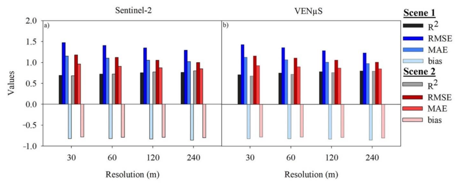
3.1.3. TsHARP Validation Comparison between VENµS and Sentinel-2

The validation results of MODIS coarse images’ thermal sharpening using VENµS VNIR was compared to results from sharpening using Setninel-2 on 28 October at scenes 1 and 2 (Figure 6). The sharpening performance using both satellites was comparable for both scenes, yielding similar temperature errors, accuracy, and bias. The relationship between sharpened and reference temperatures was strong in all instances with values ranging from 0.68 to 0.80, and temperature uncertainty ranging from 1 to 1.47 °C. Although similar, MODIS/Sentinel-2 performance was slightly higher at 120 and 240 m in scene 2 when compared to scene 1, with R2 values of 0.77 and 0.8, while VENµS sharpening showed higher accuracy in scene 1 at all four different spatial resolutions. MODIS/VENµS was also slightly more accurate than MODIS/Sentinel-2 in scene 1 in all spatial resolutions, with R2 values of 0.71 and 0.69 at 30 m, 0.75 and 0.72 at 60 m, 0.78 and 0.75 at 120 m, and 0.80 and 0.76 at 240 m resolutions for MODIS/VENµS and MODIS/Sentinel-2 respectively, while in scene 2, both models had the same R2 at 30 and 60 m, with Sentinel-2 achieving higher R2 at 120 and 240 m. Overall, scene 2 showed lower RMSE, MAE, and bias than scene 1 in both models, with highest values of 1.16, 0.93, and −0.80 for VENµS, and 1.18, 0.96, and −0.80 for Sentinel-2, respectively.

3.2. Field Scale

Field boundaries were extracted from sharpened and reference images at 30, 60, 120, and 240 m to perform validation at a field scale for each individual field. The field selection criteria relied solely on the crop cultivated. Cotton fields were identified using USDA-NASS CropScape data layer from 2019.

3.2.1. MODIS/Sentinel-2 TsHARP Validation

The validation of the sharpening algorithm in scene 2 was performed in eight fields on 9 September (Figure 7). An overall strong relationship between sharpened and reference temperatures was observed in fields 1 and 3 across all spatial resolutions, with R2 values ranging from 0.60 at 30 m to 0.94 at 240 m, and 0.64 at 30 m to 0.88 at 120 m, respectively. The weakest relationships were observed for fields 8 and 4, wherein the model’s accuracy was below 0.5 in all resolutions. Remaining fields showed strong relationships at 60, 120, and 240 m, with the exception of field 5, in which higher accuracy was obtained only at coarser resolutions of 120 and 240 m. Only three fields showed moderate to strong relationships at the finest targeted resolution, while for the other resolutions, temperature estimation results were more reliable, with most fields having higher accuracy maps. Temperature uncertainty of higher than 2 °C was obtained for fields 1, 2, and 5, while field 6 resulted in errors lower than 1 °C (Figure 7b).
The negative bias shown in all areas indicated an underestimation of BT when compared to reference data and it is consistent with the results obtained for the scene scale. The residual errors resulted from the linear regression between BT and NDVI showed errors ranging from −0.5 to 1 °C in the areas that fields were located. Nevertheless, temperature underestimation in sharpened maps was as high as 2.5 °C in some fields, likely due to a discrepancy in temperatures collected by both thermal sensors in these specific areas, rather than due to a weak relationship between BT and NDVI. This temperature difference can be a result of biases caused by sensor parameters such as bandwidth, acquisition time, and geolocation errors [32].
The field scale validation results for scene 3 are shown in Figure 8. Due to the lower number of cotton fields in this scene and their smaller size, only five fields were selected for analysis. Nevertheless, a higher number of dates throughout the growing season were available for validation.
High performances were observed in September (Figure 8b,e) and October (Figure 8c,f), in which most fields showed a strong relationship between sharpened and reference temperatures coupled with the low-temperature errors. A positive bias in September indicates that temperatures were overestimated at an average of 0.95 °C in all fields. Despite the high agreement between sharpened and reference temperatures observed for all fields in August, in one or more resolutions, temperature error was higher than in subsequent months (Figure 8a,d). Spatial resolutions of 60 and 120 m displayed the most consistent results along the three dates, with strong relationships in most fields. High R2 values were observed in four out of five fields at 60 m resolution on the second and third dates, and two fields on the first date, while at 120 m, all five fields had strong relationships on the first date, four on the third, and three on the second. Sharpened maps at 30 m had the weakest performance, with a maximum of 2 fields presenting moderate relationships and overall temperature errors higher than coarser resolutions. Maps at 240 m had weaker performance in this scene due to the low or insufficient number of pixels for correlation caused by the smaller field sizes.
The resulting statistics indicated that the thermal sharpening of coarse MODIS images at the four finer resolutions are field-specific. The accuracy of sharpened temperatures in field 5 was high at all resolutions on the first date and was consistently high at 60 and 120 m in subsequent months. High-temperature maps’ accuracy was observed in at least three resolutions at fields 2 and 3 in September and October, and at 240 m in the first month. The weakest performance was observed in field 4, in which sharpened maps had very low accuracy among all dates in most spatial resolutions when compared to Landsat reference temperatures. The fields that showed the strongest (field 5) and the weakest performances (field 4) were located side by side in the scene, suggesting that the sharpening results might be affected by field individual characteristics, planting date, and management practices.
High agreement between sharpened and reference maps at 60 m resolution was observed in field 1 for all three dates (Figure 9). Despite the higher temperature difference between sharpened and reference maps in August, the BT distribution patterns still showed great similarities. A high correlation between sharpened and reference maps was also shown on the subsequent dates. The high agreement between sharpened and reference maps shown in the validation process evidences great consistency in the TsHARP results. The robust results from the use of Sentinel-2 VNIR for sharpening presented in this study are corroborated by studies previously mentioned [19,20].

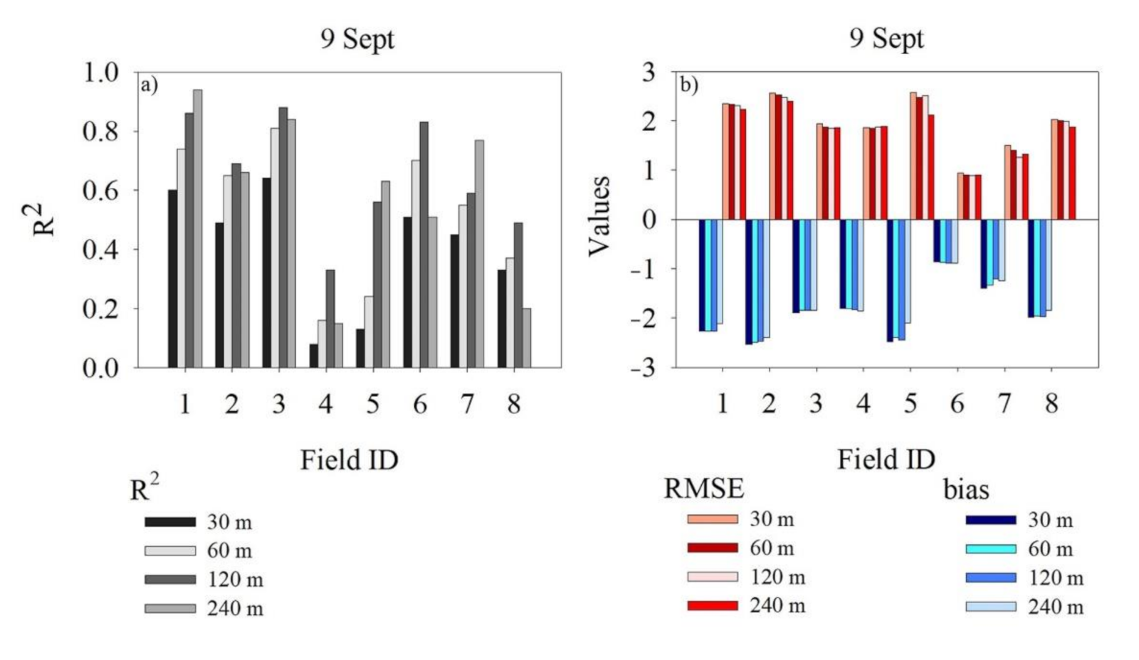
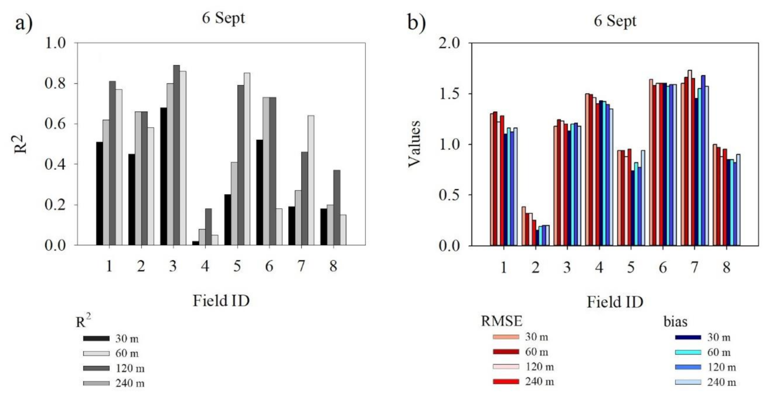
3.2.2. MODIS/VENµS TsHARP Validation

Figure 10 shows the quantitative statistics for TsHARP validation at two different dates in scene 1. The algorithm’s performance presented variability between dates and areas, as previously observed. The model’s accuracy was consistent across three out of the nine fields selected, with strong relationships in all resolutions in field 6 at both dates, and at the second date for fields 2 and 5. On 29 August, high-accuracy sharpened maps for fields 2 and 5 were observed at 60 and 120 m only. Fields 7 and 8 showed high R2 values between sharpened and reference temperatures only at the coarser resolutions of 120 and 240 m, while in remaining fields, the overall accuracy was low either on all or one of the dates. Disaggregated maps at 120, 240, and 60 m resolutions were the most consistent in terms of correlation with reference temperature maps. Temperature uncertainty was relatively low in most fields at both dates, with values ranging from 1.25 to 2.17 °C in August and 0.66 to 2.13 °C in September. An overestimation of sharpened temperatures was observed in August with a positive bias of 2.17 °C, while in September, sharpened temperatures were up to 2.01 °C lower than reference temperatures. On this date, temperature overestimation was observed only in field 4, in which sharpened temperatures were on average 0.66 °C higher than the reference.
In scene 2, the MODIS images’ sharpening using VENµS NDVI was validated on one date in the beginning of September, with three days difference from the MODIS/Sentinel-2-derived sharpened image (Figure 11). A field scale comparison between these two sharpened maps was not performed because of the time difference, however similarities in the results were observed. Fields 8 and 4 had weak relationships between sharpened and reference temperatures in all spatial resolutions, repeating the weak performance seen in the MODIS/Sentinel-2 scene. These results suggest that the poor accuracy of the sharpened maps was caused by subfield land cover variability that was not depicted in the coarse MODIS pixel resolution, such as a mix of exposed soil and canopy cover. The possible effects of different field conditions will be discussed in the next subsection.
Overall, sharpening accuracy was high at 60, 120, and 240 m, with at least half of the fields showing R2 values higher than 0.62. Only three fields had moderate to strong relationship at 30 m, with the highest value of 0.68. Overall, RMS errors were below 1.73 at all four resolutions. Temperature uncertainty as low as 0.25 °C was achieved at 240 m in field 2 and as low as 0.38 °C at 30 m. Bias indicated that sharpened temperatures were overestimated in all fields (Figure 11b). High-accuracy sharpened maps were achieved for all resolutions in field 3 (Figure 12). Sharpened map with 30 m pixel size provided the most detailed insight in the BT distribution in the field (Figure 12a). The same BT patterns were maintained when pixel size was doubled, and sharpening accuracy increased from 0.68 to 0.8 (Figure 12e,f). The two coarser maps presented even higher accuracy of 0.89 and 0.86, but temperature distribution patterns in the field became harder to identify (Figure 12c,d). Exposed soil at the northern part and in the middle of the lower half of the field, most likely caused by erosion processes over the years, resulted in an overestimation of sharpened temperatures in those pixels. In these areas, sharpened temperatures were around 30.8 °C, while in the reference image, the same pixels varied from 28 to 29 °C, causing a decrease in the overall accuracy at 30 m. Background soil reflectance can also affect the sharpening performance throughout the season, once the low vegetation cover in the first stages of crop development can lead to high amounts of mixed pixel reflectance and consequently, an overestimation of canopy sharpened temperatures.
Disaggregation methods are often studied in large scene scales. Few authors have attempted to use this methodology for small agricultural areas. Sánchez et al. [20] used Sentinel-2 to sharpen MODIS coarse thermal images to 10 m resolutions over a semi-arid agricultural area in southeast Spain. An average temperature uncertainty of 2 °C was observed. Temperature errors between 2 and 3 °C were observed by Bisquert et al. [14]. In a simulated experiment, Landsat 7 thermal images were aggregated to coarse resolution and then sharpened, achieving temperature uncertainty of ~1 °C [40]. In the present study, temperature errors for field scale ranged from 0.25 to 3.11 °C using both Sentinel-2 and VENµS, following results found by the other authors. Furthermore, it has been reported that absolute temperature errors of up to 1.5 °K are suitable for agricultural management decisions [20,41,42]. Results from this paper are encouraging. A great number of fields presented low errors at 240 and 120 m, and at the finer resolutions of 60 m and in lesser cases of 30 m. The high-accuracy maps generated from this methodology with relatively low errors show a great potential in the use of TsHARP in MODIS/Sentinel-2 and MODIS/VENµS combinations for field scale.
Figure 13 shows field 3 sharpened temperature distribution in relation to air temperature on 5 days throughout the growing season from June to September at 60 m resolution. Air-canopy temperature difference is a well-recognized indicator of water stress in cotton [43,44]. Field canopy temperatures in June were less than 3 °C below air temperature, while in August and September, this difference was as high as 5 °C. Air-canopy temperature distribution was very similar throughout the field in the first and last dates. In the dates from mid-June to early September, a slight variability in air-canopy temperature distribution is observed. The use of a high spatial resolution satellite such as VENµS with high revisit time to sharpen coarse thermal images presents great potential to enable a more frequent monitoring of canopy temperature changes across the field throughout the growing season, with a fine resolution with the aim to identify crop water stress patterns in the field for management zone delineation. It is important to note that for a better estimation of plant water status, the sharpened BT values should be converted to LST [45].

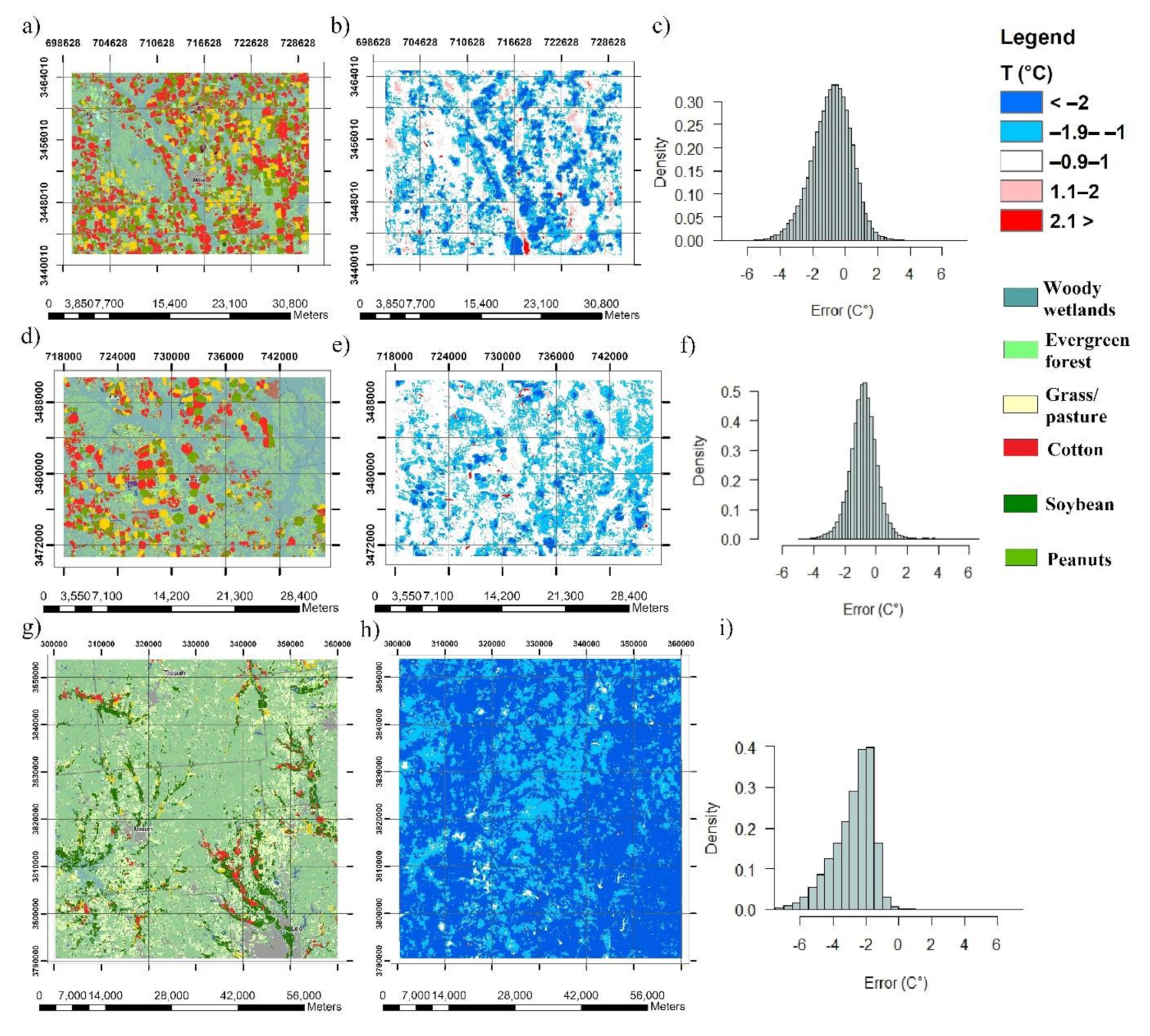
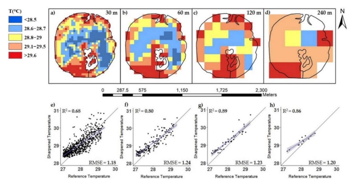
3.2.3. Effects of In-Field Land Cover Variability on TsHARP Performance

Two fields from scene 1 in Miller county were selected to demonstrate how different field conditions can positively or negatively affect the accuracy of resulting sharpened maps in a field scale. Figure 14 shows an example of the comparison between before and after exclusion of selected areas within fields 3 and 9. Land patches covered by vegetation other than the cultivated crop, roads, flow channels caused by erosion, exposed soil, and waterlogged areas were extracted from the field boundaries for validation (Figure 14e–h). These areas were usually responsible for decreasing the level of accuracy between reference (Figure 14a,c) and sharpened (Figure 14b,d) maps. This difference was likely caused by the sharpening technique reliance on the BT–NDVI relationship, once many of these land cover types mentioned have low NDVI values resulting in high sharpened temperatures, while reference images are dependent on the temperature variability itself and not on the NDVI patterns throughout the area.
Reference and sharpened maps after the pixel removal process of fields 3 and 9 are shown in Figure 14i–l. Note that the temperature distribution at sharpened and reference maps appear to become more alike in field 3 after removal of unwanted pixels. A circular area around the pivot, a narrow road, and a waterlogged area were excluded in this field, increasing the sharpening accuracy. This stronger relationship between the two maps was likely due to two factors: (1) exposed soil pixels from the road had low NDVI values, resulting in finer pixels with overestimated temperature at the sharpened map, and (2) the two remaining excluded areas had high moisture, which explains the lower temperature relative to the rest of the field in the reference map, while in the sharpened map, pixel temperatures were higher in these areas than in the remaining field due to the low NDVI values of water patches and wet soil. Conversely, the extraction process did not yield the same results for field 9 once BT pattern differences were still evident in the remainder of the field. Based on the temperature range in the reference image and on the premise that stressed cotton plants are usually up to 5 °C above air temperature [46,47], it is possible to infer that the whole field was well-watered either due to rain or irrigation events. The TsHARP algorithm may not detect the moisture variability caused by irrigation, since it accounts for the subpixel temperature variability related to the vegetation fraction, thus making irrigation events a common source of error [40].
Although little information about most of the fields studied is known, it can be assumed that field-specific conditions are a determinant factor in the accuracy of sharpened temperatures. For instance, different authors have pointed out the limitations of thermal disaggregation in irrigated fields [14,48]. Surface temperature can rapidly respond to water stress, while NDVI has a slower response after initial stress [36]. Agam et al. [40] discussed the importance of excluding selected pixels that do not conform to the inverse linear relationship between LST and vegetation fraction, such as water bodies that present both low NDVI and surface temperature. Furthermore, areas that have high NDVI variability may be a source of errors once this variability cannot be depicted by the coarse resolution pixels of MODIS images.
Temperature data from field 9 collected with Landsat resulted in higher temperature along the entire west edge of the field, potentially due to a mixed pixel response between the crop and the grassed area adjacent to the field. However, vegetation cover in the same area was high, leading to an opposing result in the sharpened image. The observations on the effect of undesirable pixels’ removal on the thermal pixel disaggregation performance are reinforced by statistics shown in Figure 15. A higher level of agreement between the sharpened and reference temperatures was displayed after pixel extraction in field 3 on both dates, as well as a decrease in temperature errors, whereas in field 9, the accuracy decreased at 30 and 120 m, despite slightly lower errors being achieved.

4. Conclusions

Corroborating findings found in the literature, results from this study highlighted the differences in coarse-resolution BT between MODIS and Landsat. For the five dates for which imagery from both sensors were acquired on the same day, observed average MAE was 1.63 °C. Coefficient of determination within the same dates varied from 0.34 to 0.74, with scene MODIS BT frequently being cooler than Landsat-8. Further research can benefit from implementation of intercalibration between MODIS and Landsat-8 before sharpening validation to attenuate errors caused by the sensors’ individual characteristics. Despite the inconsistent correlations in coarse resolution caused by these differences and the presence of clouds in one or both images, relationships between sharpened MODIS and Landsat were stronger at all finer resolutions.
Field-scale agreement between sharpened and reference temperatures showed some level of independence from the scene scale. Agricultural fields located in regions of the scene with smaller residual errors or not affected by cloud cover can show higher temperature accuracy than other areas. These findings suggest that sharpened maps can be used with caution for small scales even if coarse comparison between sensors in the scene scale shows weaker relationships.
Sharpened maps at 120 and 60 m resolution showed the highest consistency within all fields and dates using both VENµS and Sentinel-2. Maps sharpened to 240 m showed high accuracy, but greatly depended on the field size because of the lack of pixels available in smaller areas. Resolutions finer than 60 m presented the least consistent relationships, with accurate maps being very field-specific.
Very few studies have explored the performance of thermal sharpening in field scales, and the use of VENµS multispectral data. Findings from this research show that considering the combination of pixel size, and temperature estimation accuracy and error, sharpened MODIS at 60 m are the most reliable for season-long cotton monitoring. The comparison between sharpened images using VENµS and Sentinel-2 was performed to evaluate a potential agreement between results, due to the lack of information available in the use of VENµS for thermal disaggregation. VENµS results showed comparable or higher accuracy than Sentinel-2. The superior performance coupled with the better revisit time evidences the great potential of using VENµS for frequent in-season crop monitoring for IMZ delineation.
This work is the first to report the use of VENµS images for thermal sharpening. Nevertheless, only an initial study was performed to explore the possibility of using sharpening at field scale for monitoring purposes. Further research with ground data collection is needed to explore field use limitations of this methodology, but these results give useful insights of potential benefits of implementing the TsHARP technique as a tool for crop stress monitoring.

Author Contributions

The contribution of authors are as follows: conceptualization, Y.C. and H.H.; methodology, Y.C. and H.H; software, L.N.L. and H.H.; validation, L.N.L. and H.H.; formal analysis, L.N.L.; writing—original draft preparation, L.N.L.; writing—review and editing, Y.C., J.S., V.L., and G.V.; visualization, L.N.L., Y.C., J.S., H.H., V.L., and G.V.; funding acquisition, Y.C., J.S., V.L., and G.V. All authors have read and agreed to the published version of the manuscript.

Funding

This research was funded by US-Israel Binational Research and Development Fund (BARD) Research Project US-4991-1.

Acknowledgments

The authors thank the Israel Space Agency for providing us images from the VENµS mission.

Conflicts of Interest

The authors declare no conflict of interest.

Appendix A. Coordinates and Area of All Fields Selected for This Study

Table A1. List of study sites and cotton fields for all three locations.
LocationField IDCoordinatesArea (ha)
Miller County,
Georgia
(scene 1)
131°11′53″N, 84°45′45″W63.03
231°13′3″N, 84°35′2″W26.21
331°05′55″N, 84°43′27″W164.40
431°06′37″N, 84°43′35″W78.93
531°08′31″N, 84°36′01″W88.44
631°07′06″N, 84°45′34″W33.14
731°07′50″N, 84°52′26″W32.30
831°06′21″N, 84°51′45″W35.68
931°11′20″N, 84°45′41″W38.20
--------------------
Baker County,
Georgia
(scene 2)
131°26′17″N, 84°36′02″W66.80
231°28′38″N, 84°39′46″W59.07
331°26′17″N, 84°36′38″W63.11
431°26′27″N, 84°34′34″W48.30
531°23′55″N, 84°32′53″W58.45
631°27′51″N, 84°28′08″W56.74
731°28′46″N, 84°29′30″W33.47
831°28′01″N, 84°33′24″W90.91
--------------------
Union County,
Mississippi
(scene 3)
134°21′40″N, 89°08′10″W89.91
234°48′05″N, 88°56′42″W14.05
334°24′07″N, 88°45′16″W84.44
434°20′04″N, 89°01′27″W34.36
534°19′57″N, 89°01′12″W16.97

References

  1. Ishimwe, R.; Abutaleb, K.; Ahmed, F. Applications of Thermal Imaging in Agriculture—A review. Adv. Rem. Sens. 2014, 3, 128–140. [Google Scholar] [CrossRef] [Green Version]
  2. Ribeiro da Luz, B. Attenuated total reflectance spectroscopy of plant leaves: A tool for ecological and botanical studies. New Phytol. 2006, 172, 305–318. [Google Scholar] [CrossRef] [PubMed]
  3. Hsiao, T. Plant Responses to water stress. Ann. Rev. Plant Physiol. 1973, 24, 519–570. [Google Scholar] [CrossRef]
  4. Bodner, G.; Nakhforoosh, A.; Kaul, H.-P. Management of crop water under drought: A review. Agron. Sustain. Dev. 2015, 35, 401–442. [Google Scholar] [CrossRef]
  5. Falkenberg, N.R.; Piccinni, G.; Cothren, J.T.; Leskovar, D.I.; Rush, C.M. Remote sensing of biotic and abiotic stress for irrigation management of cotton. Agric. Water Manag. 2007, 87, 23–31. [Google Scholar] [CrossRef]
  6. Costa, J.O.; Coelho, R.D.; Barros, T.H.S.; Junior, E.F.F.; Fernandes, A.L.T. Canopy thermal responses to water deficit of coffee plants under drip irrigation. Irrig. Drain. 2020, 69, 472–482. [Google Scholar] [CrossRef]
  7. Panigada, C.; Rossini, M.; Meroni, M.; Cilia, C.; Busetto, L.; Amaducci, S.; Boschetti, M.; Cogliati, S.; Picchi, V.; Pinto, F.; et al. Fluorescence, PRI and canopy temperature for water stress detection in cereal crops. Int. J. Appl. Earth Obs. Geoinf. 2014, 30, 167–178. [Google Scholar] [CrossRef]
  8. Elsayed, S.; Elhoweity, M.; Ibrahim, H.H.; Dewir, Y.H.; Migdadi, H.M.; Schmidhalter, U. Thermal imaging and passive reflectance sensing to estimate the water status and grain yield of wheat under different irrigation regimes. Agric. Water Manag. 2017, 189, 98–110. [Google Scholar] [CrossRef]
  9. O’Shaughnessy, S.A.; Evett, S.R.; Colaizzi, P.D.; Howell, T.A. Using radiation thermography and thermometry to evaluate crop water stress in soybean and cotton. Agric. Water Manag. 2011, 98, 1523–1535. [Google Scholar] [CrossRef]
  10. Cohen, Y.; Alchanatis, V.; Saranga, Y.; Rosenberg, O.; Sela, E.; Bosak, A. Mapping water status based on aerial thermal imagery: Comparison of methodologies for upscaling from a single leaf to commercial fields. Precis. Ag. 2017, 18, 801–822. [Google Scholar] [CrossRef]
  11. Agam, N.; Kustas, W.P.; Anderson, M.C.; Li, F.; Neale, C.M.U. A vegetation index based technique for spatial sharpening of thermal imagery. Remote Sens. Environ. 2007, 107, 545–558. [Google Scholar] [CrossRef]
  12. Cohen, Y.; Agam, M.; Klapp, I.; Karnieli, A.; Beeri, O.; Alchanatis, V.; Sochen, N. Future approaches to facilitate large-scale adoption of thermal based images as key input in the production of dynamic irrigation management zones. Adv. Anim. Biosci. 2017, 8, 546–550. [Google Scholar] [CrossRef]
  13. Zhan, W.; Chen, Y.; Zhou, J.; Wang, J.; Liu, W.; Voogt, J.; Zhu, X.; Quan, J.; Li, J. Disaggregation of remotely sensed land surface temperature: Literature survey, taxonomy, issues, and caveats. Remote Sens. Environ. 2013, 131, 119–139. [Google Scholar] [CrossRef]
  14. Bisquert, M.; Sanchez, J.M.; Caselles, V. Evaluation of Disaggregation Methods for Downscalling MODIS Land Surface Temperature to Landsat Spatial Resolution in Barrax Test Site. IEEE J. Sel. Top. Appl. Earth Obs. Remote Sens. 2016, 9, 1430–1438. [Google Scholar] [CrossRef]
  15. Tom, V.T.; Carlotto, M.J.; Scholten, D.K. Spatial Sharpening of Thematic Mapper Data Using a Multiband Approach. Opt. Eng. 1985, 24, 1026–1029. [Google Scholar] [CrossRef]
  16. Kustas, W.P.; Norman, J.M.; Anderson, M.C.; French, A.N. Estimating subpixel surface temperatures and energy fluxes from the vegetation index-radiometric temperature relationship. Remote Sens. Environ. 2003, 85, 429–440. [Google Scholar] [CrossRef]
  17. Bindhu, V.M.; Narasimhan, B.; Sudheer, K.P. Development and verification of a non-linear disaggregation method (NL-DisTrad) to downscale MODIS land surface temperature to the spatial scale of Landsat thermal data to estimate evapotranspiration. Remote Sens. Environ. 2013, 135, 118–129. [Google Scholar] [CrossRef]
  18. Wang, R.; Gao, W.; Peng, W. Downscale MODIS Land Surface Temperature Based on Three Different Models to Analyze Surface Urban Heat Island: A Case Study of Hangzhou. Remote Sens. 2020, 12, 2134. [Google Scholar] [CrossRef]
  19. Huryna, H.; Cohen, Y.; Karnieli, A.; Panov, N.; Kustas, W.; Agam, N. Evaluation of TsHARP Utility for Thermal Sharpening of Sentinel-3 Satellite Images Using Sentinel-2 Visual Imagery. Remote Sens. 2019, 11, 2304. [Google Scholar] [CrossRef] [Green Version]
  20. Sánchez, J.M.; Galve, J.M.; González-Piqueras, J.; López-Urrea, R.; Niclòs, R.; Calera, A. Monitoring 10-m LST from the Combination MODIS/Sentinel-2, Validation in a High Contrast Semi-Arid Agroecosystem. Remote Sens. 2020, 12, 1453. [Google Scholar] [CrossRef]
  21. Ferrier, P.; Crebassol, P.; Dedieu, G.; Hagolle, O.; Meygret, A.; Tinto, F.; Yaniv, Y.; Herscovitz, J. VENµS (Vegetation and Environment Monitoring on A New Micro Satellite). In Proceedings of the Institute of Electrical and Electronics Engineers (IEEE) International Geoscience Remote Sensing Symposium, Honolulu, HI, USA, 25–30 July 2010; pp. 3736–3739. [Google Scholar] [CrossRef]
  22. Sharing Earth Obeservation Resources eoPortal Directory. Available online: https://directory.eoportal.org/web/eoportal/satellite-missions/v-w-x-y-z/venus (accessed on 25 August 2020).
  23. Kottek, M.; Grieser, J.; Beck, C.; Rudolf, B.; Rubel, F. World Map of the Köppen-Geiger climate classification updated. Meteorol. Z. 2006, 15, 259–263. [Google Scholar] [CrossRef]
  24. Beck, H.; Zimmermann, N.; McVicar, T.; Vergopolan, N.; Berg, A.; Wood, E. Present and future Köppen-Geiger climate classification maps at 1-km resolution. Sci. Data 2018, 5, 1–12. [Google Scholar] [CrossRef] [Green Version]
  25. NOAA National Centers for Environmental information, Climate at a Glance: Regional Time Series, Published December 2020. Available online: https://www.ncdc.noaa.gov/cag/ (accessed on 23 December 2020).
  26. Boryan, C.; Yang, Z.; Mueller, R.; Craig, M. Monitoring US agriculture: The US Department of Agriculture, National Agricultural Statistics Service, Cropland Data Layer Program. Geocarto Intern. 2011, 26, 341–358. [Google Scholar] [CrossRef]
  27. MODTBGA MODIS/Terra Thermal Bands Daily L2G-Lite Global 1 km SIN Grid V006. Available online: https://lpdaac.usgs.gov/products/modtbgav006/ (accessed on 24 August 2020).
  28. QGIS Development Team. QGIS Geographic Information System; Open Source Geospatial Foundation: Beaverton, OR, USA, 2020. [Google Scholar]
  29. Leroux, L.; Congedo, L.; Bellón, B.; Gaetano, R.; Bégué, A. Land Cover Mapping Using Sentinel-2 Images and the Semi-Automatic Classification Plugin: A Northern Burkina Faso Case Study. In QGIS and Application in Agriculture and Forest; Baghdadi, N., Mallet, C., Zribi, M., Eds.; Wiley: Hoboken, NJ, USA, 2018; pp. 119–151. [Google Scholar]
  30. Choudhury, B.; Ahmed, N.; Idso, S.; Reginato, R.; Daughtry, C. Relations between evaporation coefficients and vegetation indices studied by model simulations. Remote Sens. Environ. 1994, 50, 1–17. [Google Scholar] [CrossRef]
  31. Willmott, C.J. Some Comments on the Evaluation of Model Performance. Bull. Am. Meteorol. Soc. 1982, 63, 1309–1313. [Google Scholar] [CrossRef] [Green Version]
  32. Weng, Q.; Fu, P.; Gao, F. Generating daily land surface temperature at Landsat resolution by fusing Landsat and MODIS data. Remote Sens. Environ. 2014, 145, 55–67. [Google Scholar] [CrossRef]
  33. Essa, W.; Verbeiren, B.; Van Der Kwast, J.; Batelaan, O. Improved DisTrad for Downscaling Thermal MODIS Imagery over Urban Areas. Remote Sens. 2017, 9, 1243. [Google Scholar] [CrossRef] [Green Version]
  34. Liu, Y.; Hiyama, T.; Yamaguchi, Y. Scaling of land surface temperature using satellite data: A case examination on ASTER and MODIS products over a heterogenous terrain area. Remote Sens. Environ. 2006, 105, 115–128. [Google Scholar] [CrossRef]
  35. Chen, X.; Li, W.; Chen, J.; Rao, Y.; Yamaguchi, Y. A Combination of TsHARP and Thin Plate Spline Interpolation for Spatial Sharpening of Thermal Imagery. Remote Sens. 2014, 6, 2845–2863. [Google Scholar] [CrossRef] [Green Version]
  36. Sandholt, I.; Rasmussen, K.; Andersen, J. A simple interpretation of the surface temperature/vegetation index space for assessment of surface moisture status. Remote Sens. Environ. 2002, 79, 213–224. [Google Scholar] [CrossRef]
  37. Anderson, M.C.; Allen, R.G.; Morse, A.; Kustas, W.P. Use of Landsat thermal imagery in monitoring evapotranspiration and managing water resources. Remote Sens. Environ. 2012, 122, 50–65. [Google Scholar] [CrossRef]
  38. Karnieli, A.; Agam, N.; Pinker, R.T.; Anderson, M.; Imhoff, M.L.; Gutman, G.G.; Panov, N.; Goldberg, A. Use of NDVI and Land Surface Temperature for Drought Assessment: Merits and Limitations. J. Clim. 2010, 23, 618–633. [Google Scholar] [CrossRef]
  39. Li, X.; Xin, X.; Jiao, J.; Peng, Z.; Zhang, H.; Shao, S.; Liu, Q. Estimating Subpixel Surface Heat Fluxes through Applying Temperature-Sharpening Methods to MODIS Data. Remote Sens. 2017, 9, 836. [Google Scholar] [CrossRef] [Green Version]
  40. Agam, N.; Kustas, W.P.; Anderson, M.C.; Li, F.; Colaizzi, P.D. Utility of thermal sharpening over Texas high plains irrigated agricultural fields. J. Geophys. Res. 2007, 112, D19110. [Google Scholar] [CrossRef] [Green Version]
  41. Sobrino, J.A.; Jiménez-Muñoz, J.C.; Sòria, G.; Ruescas, A.B.; Danne, O.; Brockmann, C.; Ghent, D.; Remedios, J.; North, P.; Merchant, C.; et al. Synergistic use of MERIS and AATSR as a proxy for estimating Land Surface Temperature from Sentinel-3 data. Remote Sens. Environ. 2016, 179, 149–161. [Google Scholar] [CrossRef]
  42. Ghent, D.J.; Corlett, G.K.; Remedio, J.J. Global Land Surface Temperature From the Along-Track Scanning Radiometers. J. Geophys. Res. Atmos. 2017, 122, 12167–12193. [Google Scholar] [CrossRef] [Green Version]
  43. Jackson, R.D.; Idso, S.B.; Reginato, R.J.; Pinter, P.J., Jr. Canopy Temperature as a Crop Water Stress Indicator. Water Resour. Res. 1981, 17, 1133–1138. [Google Scholar] [CrossRef]
  44. Wanjura, D.F.; Upchurch, D.R. Canopy temperature characterizations of corn and cotton water stress. Trans. ASAE 2000, 43, 867–875. [Google Scholar] [CrossRef]
  45. Li, F.; Jackson, T.J.; Kustas, W.P.; Schmugge, T.J.; French, A.N.; Cosh, M.H.; Bindlish, R. Deriving land surface temperature from Landsat 5 and 7 during SMEX02/SMACEX. Remote Sens. 2004, 92, 521–534. [Google Scholar] [CrossRef]
  46. Idso, S.B.; Jackson, R.D.; Pinter, P.J., Jr.; Reginato, R.J.; Hatfield, J.L. Normalizing the stress-degree-day parameter for environmental variability. Agric. Meteorol. 1981, 24, 45–55. [Google Scholar] [CrossRef]
  47. Cohen, Y.; Alchanatis, V.; Meron, Y.; Saranga, Y.; Tsipris, J. Estimation of leaf water potential by thermal imagery and spatial analysis. J. Exp. Bot. 2005, 56, 1843–1852. [Google Scholar] [CrossRef] [Green Version]
  48. Merlin, O.; Duchemin, B.; Hagolle, O.; Jacob, F.; Coudert, B.; Chehbouni, G.; Dedieu, G.; Garatuza, J.; Kerr, Y. Disaggregation of MODIS surface temperature over an agricultural area using a time series of Formosat-2 images. Remote Sens. Environ. 2010, 114, 2500–2512. [Google Scholar] [CrossRef] [Green Version]
Figure 1. Study locations for (a) the polygons used to define the satellite scenes and Sentinel-2 false color composite of scenes used for thermal sharpening for study sites in (b) Miller County, Georgia (Scene 1) (c) Baker County, Georgia (Scene 2) and (d) Union County, Mississippi (Scene 3).
Remotesensing 13 01155 g001
Figure 2. Flowchart of the thermal sharpening (TsHARP) methodology, including inputs, outputs, and processing steps, and methodology validation using Landsat-8 images (modified after Huryna et al. [19]).
Remotesensing 13 01155 g002
Figure 3. Relationship between MODIS BT and Landsat-8 BT at coarse resolution (930 m) in selected periods for Sentinel-2 at (a) scene 1 (Miller County, GA, USA), (b) scene 2 (Baker County, GA, USA), and (c) scene 3 (Union County, MS, USA). MODIS acquisition dates were used as the reference date.
Remotesensing 13 01155 g003
Figure 4. Relationship between MODIS BT and Landsat-8 BT at coarse resolution (930 m) in selected periods for VENµS at (a) scene 1 and (b) scene 2. MODIS acquisition dates were used as the reference date.
Remotesensing 13 01155 g004
Figure 5. Land cover maps of (a) scene 1, (d) scene 2, and (g) scene 3, (b,e,h) are the respective temperature error maps (sharpened T (°C) − reference T (°C)) at 60 m resolution, and (c,f,i) are the respective error histograms. Error maps/histograms presented were created from MODIS/Sentinel-2 sharpening from the last date of scenes 1 and 2, and first date of scene 3.
Remotesensing 13 01155 g005
Figure 6. Quantitative statistics of TsHARP validation yielded by MODIS sharpening using (a) scheme 2 and (b) VENµS at scenes 1 and 2.
Remotesensing 13 01155 g006
Figure 7. Quantitative statistics between sharpened and reference temperatures at field scale for fields selected in scene 2, including (a) coefficient of determination (b) RMSE, and bias.
Remotesensing 13 01155 g007
Figure 8. Quantitative statistics between sharpened and reference temperatures at field scale for fields selected in scene 3 on three different dates, including coefficient of determination on (a) 29 August (b) 15 September and (c) 3 October, and (df) RMSE and bias for the same dates, respectively.
Remotesensing 13 01155 g008
Figure 9. Field 1 sharpened temperature maps at 60 m resolution in Mississippi on (a) 29 August (b) 15 September and (c) 3 October, in comparison with respective (df) reference temperature maps. (gi) Temperature error maps (sharpened T (°C)–reference T (°C)) for each date at 60 m resolution. Quantile method was used for classification.
Remotesensing 13 01155 g009
Figure 10. Quantitative statistics between sharpened and reference temperatures at field scale for fields selected in scene 1 including coefficient of determination, (a) 29 August and (b) 10 September, and (c,d) RMSE and bias for respective dates.
Remotesensing 13 01155 g010
Figure 11. Quantitative statistics between sharpened and reference temperatures at field scale for fields selected in scene 2 including (a) coefficient of determination and (b) RMSE and bias.
Remotesensing 13 01155 g011
Figure 12. Field 3 sharpening maps of MODIS images using VENµS at (a) 30 (b) 60 (c) 120 and (d) 240 m resolution, and (eh) the respective validation regressions.
Remotesensing 13 01155 g012
Figure 13. Field 3 time series of canopy temperature (Tc) - air temperature (Tair) distribution throughout the season. Canopy temperature used was extracted from the sharpened temperature maps.
Remotesensing 13 01155 g013
Figure 14. Field map comparison between reference and sharpened (MODIS/VENµS) maps before and after pixel removal. (ad) Reference and sharpened maps of the whole area within fields 3 and 9. (eh) Visual imagery and field boundary for both fields. (il) Reference and sharpened maps after pixel extraction for fields 3 and 9.
Remotesensing 13 01155 g014
Figure 15. Fields 3 and 9 comparison statistics between sharpened and reference temperatures before and after pixel removal on 29 August and 10 September, including (a) coefficient of determination and (b) RMSE.
Remotesensing 13 01155 g015
Table 1. Satellites’ data acquisition dates for all three locations and selected dates for field scale validation of the Moderate Resolution Imaging Spectrometer MODIS for both Sentinel-2 and VENµS (gray).
LocationLandsat-8MODISSentinel-2VENµS
Acquisition Date
Miller County24 August 201929 August 2019-29 August 2019
Georgia09 September 201910 September 2019-10 September 2019
(scene 1)25 September 201924 September 201924 September 2019-
27 October 201928 October 201927 October 201928 October 2019
--------------------
Baker County09 September 20196 September 2019-6 September 2019
Georgia09 September 201909 September 201909 September 2019-
(scene 2)25 September 201924 September 201924 September 2019-
27 October 201928 October 201927 October 201928 October 2019
--------------------
Union, County29 August 201929 August 201929 August 2019-
Mississippi14 September 201915 September 201915 September 2019-
(scene 3)30 September 20193 October 20193 October 2019-
1 November 20192 November 20192 November 2019-
Table 2. Scene minimum, maximum, and temperature ranges for MODIS (1 km) and Landsat-8 (30 m) original images.
SatelliteLocationMODIS Landsat-8
DateMinmaxRangeLag (days)DateminmaxRange
Sentinel-2Scene 124 Sept.27.031.94.9+125 Sept.27.635.98.3
28 Oct.21.027.26.2−127 Oct.21.029.58.5
--------------------
Scene 29 Sept.23.827.73.909 Sept.25.330.75.4
24 Sept.24.532.47.9+125 Sept.28.336.48.1
28 Oct.20.125.04.9−127 Oct.20.928.27.3
--------------------
Scene 329 Aug.21.726.04.3029 Aug.23.632.48.8
15 Sept.24.230.56.3−114 Sept.21.929.98
3 Oct.24.128.84.7−330 Sept.23.030.97.9
2 Nov.11.217.26.0−11 Nov.7.314.57.2
--------------------
VENµSScene 129 Aug.24.927.52.6−524 Aug.23.026.53.5
10 Sept.24.929.95.0−19 Sept.26.333.67.3
28 Oct.21.027.46.4027 Oct.21.029.58.5
--------------------
Scene 206 Sept.27.331.34.0+309 Sept.26.030.94.9
28 Oct.20.125.04.9−127 Oct.20.928.07.1
Landsat-8 acquisition time-scenes 1 and 2: 16:13 h, scene 3: 16:31 h; MODIS acquisition time: 100:05 h.
Table 3. Quantitative analysis of sharpened thermal maps using VENµS-derived normalized difference vegetation index (NDVI) in comparison to reference images from Landsat. Lag shows the difference in days between sharpened and Landsat-8 images.
SceneDateLagResolutionVENµS
R2RMSEMAEbias
129 August 2019−5300.481.701.571.48
600.511.691.571.48
1200.521.671.561.48
2400.491.631.531.47
10 September 2019 *−1300.522.372.12−2.09
600.542.312.07−2.03
1200.532.262.02−1.98
2400.492.201.98−1.94
28 October 20190300.711.431.13−0.82
600.751.361.07−0.82
1200.781.291.01−0.83
2400.801.230.98−0.85
--------------------
26 September 2019 *+3300.591.461.221.14
600.631.411.201.14
1200.661.371.191.14
2400.671.321.171.13
28 October 2019−1300.681.160.93−0.78
600.721.110.90−0.78
1200.761.060.87−0.79
2400.791.010.85−0.80
* Scenes with areas removed because of cloud cover.
Table 4. Quantitative analysis of sharpened thermal maps using Sentinel-2-derived NDVI in comparison to reference images from Landsat. Lag shows the difference in days between sharpened and Landsat-8 images.
SceneDateLagResolutionSentinel-2
R2RMSEMAEBias
124 September 2019 *+1300.552.141.71−1.44
600.572.111.69−1.45
1200.582.071.66−1.45
2400.552.011.63−1.48
28 October 2019−1300.691.471.15−0.82
600.721.411.10−0.82
1200.751.351.05−0.83
2400.761.291.02−0.86
--------------------
29 September 2019 *0300.601.961.78−1.77
600.641.941.77−1.77
1200.641.931.77−1.77
2400.631.911.78−1.77
24 September 2019+1300.562.812.49−2.43
600.592.772.49−2.43
1200.612.742.48−2.44
2400.612.712.48−2.46
28 October 2019−1300.681.180.96−0.78
600.721.120.91−0.79
1200.771.050.87−0.79
2400.801.000.85−0.80
--------------------
329 August 20190300.503.062.79−2.79
600.553.052.79−2.79
1200.593.032.79−2.79
2400.603.022.81−2.81
15 September 2019 *−1300.571.961.711.67
600.621.921.701.67
1200.641.871.681.65
2400.661.811.651.62
3 October 2019 *−3300.451.451.15−0.52
600.481.431.13−0.50
1200.491.401.12−0.48
2400.481.351.09−0.45
2 November 2019−1300.643.853.673.67
600.693.823.663.66
1200.743.763.653.65
2400.773.713.613.61
* Scenes with areas removed because of cloud cover.
Publisher’s Note: MDPI stays neutral with regard to jurisdictional claims in published maps and institutional affiliations.

