Abstract
Site-specific irrigation management for perennial crops such as grape requires water use assessments at high spatiotemporal resolution. In this study, small unmanned-aerial-system (UAS)-based imaging was used with a modified mapping evapotranspiration at high resolution with internalized calibration (METRIC) energy balance model to map water use (UASM-ET approach) of a commercial, surface, and direct-root-zone (DRZ) drip-irrigated vineyard. Four irrigation treatments, 100%, 80%, 60%, and 40%, of commercial rate (CR) were also applied, with the CR estimated using soil moisture data and a non-stressed average crop coefficient of 0.5. Fourteen campaigns were conducted in the 2018 and 2019 seasons to collect multispectral (ground sampling distance (GSD): 7 cm/pixel) and thermal imaging (GSD: 13 cm/pixel) data. Six of those campaigns were near Landsat 7/8 satellite overpass of the field site. Weather inputs were obtained from a nearby WSU-AgWeatherNet station (1 km). First, UASM-ET estimates were compared to those derived from soil water balance (SWB) and conventional Landsat-METRIC (LM) approaches. Overall, UASM-ET (2.70 ± 1.03 mm day−1 [mean ± std. dev.]) was higher than SWB-ET (1.80 ± 0.98 mm day−1). However, both estimates had a significant linear correlation (r = 0.64–0.81, p < 0.01). For the days of satellite overpass, UASM-ET was statistically similar to LM-ET, with mean absolute normalized ET departures (ETd,MAN) of 4.30% and a mean r of 0.83 (p < 0.01). The study also extracted spatial canopy transpiration (UASM-T) maps by segmenting the soil background from the UASM-ET, which had strong correlation with the estimates derived by the standard basal crop coefficient approach (Td,MAN = 14%, r = 0.95, p < 0.01). The UASM-T maps were then used to quantify water use differences in the DRZ-irrigated grapevines. Canopy transpiration (T) was statistically significant among the irrigation treatments and was highest for grapevines irrigated at 100% or 80% of the CR, followed by 60% and 40% of the CR (p < 0.01). Reference T fraction (TrF) curves established from the UASM-T maps showed a notable effect of irrigation treatment rates. The total water use of grapevines estimated using interpolated TrF curves was highest for treatments of 100% (425 and 320 mm for the 2018 and 2019 seasons, respectively), followed by 80% (420 and 317 mm), 60% (391 and 318 mm), and 40% (370 and 304 mm) of the CR. Such estimates were within 5% to 11% of the SWB-based water use calculations. The UASM-T-estimated water use was not the same as the actual amount of water applied in the two seasons, probably because DRZ-irrigated vines might have developed deeper or lateral roots to fulfill water requirements outside the irrigated soil volume. Overall, results highlight the usefulness of high-resolution imagery toward site-specific water use management of grapevines.
1. Introduction
Wine grape production at the desired quantity and quality is critical for commercial growers, factors that are strongly influenced by irrigation management. Vineyards are mostly located in arid and semi-arid regions that receive low rainfall and are irrigated using under-vine surface drip systems. Drip irrigation allows the flexibility of adequate irrigation during the vegetative growth stages to increase yields and deficit irrigation in later stages in order to improve grape quality, sugar content, pigment formation, and acidity [1,2]. Mapping of vine-level crop water use, i.e., evapotranspiration (ET), and pertinent spatial variation in commercial production is critical for irrigation management. In the absence of large-scale precision ET-mapping techniques, growers rely on destructive plant- and field-intensive methods such as leaf water potential [3], sap flow sensing [4,5], and soil moisture measurements [6]. Methods based on eddy covariance systems [7,8] or interpolated standard crop coefficients with reference ET from local weather data [9] are also useful. However, these methods can be laborious and costly and often lack needed sampling resolution for precision irrigation management [10].
Satellite-based remote sensing and energy balance models provide regional-scale estimates of actual ET [11]. One such model is mapping evapotranspiration at high resolution with internalized calibration (METRIC) [12,13,14]), which utilizes Landsat 5, 7, and 8 and Terra and Aqua multispectral and thermal infrared imagery inputs to compute ET as an energy balance residue within a blending height (200 m above ground level (AGL)). METRIC is independent of surface specifics, performs stabilized sensible heat flux (H) computations, and performs internal calibrations based on hot (dry bare soil) and cooler (well-irrigated vegetation) surface temperature anchor pixels to compensate computation and input measurement biases [12,15,16]. Globally, satellite-based METRIC has been shown to reliably estimate ET for a range of field and tree fruit crops in different agroclimatic zones [11,17]. Studies have reported maximum ET estimation errors of 5% for heterogeneous olive orchards compared against sap flow, soil water balance (SWB), and eddy covariance estimates [18,19,20,21], 16% for a drip-irrigated apple orchard [22], and 15% for vineyards when compared against eddy covariance fluxes [15,23].
The conventional METRIC model uses high-orbital satellite imagery to provide ET maps at low spatial (~30 m/pixel for Landsat) and temporal resolution (~16 days for Landsat). Cloud interference is an additional major challenge that restricts timely ET mapping during the crop-growing season [16,17]. Low spatiotemporal resolution may also limit ET estimation in sparse crops or vineyards irrigated by drip or similar localized methods and non-irrigated inter-row regions [24,25,26].
Subsurface irrigation, where water is applied at direct-root-zone (DRZ) depths of grapevines, has been reported to improve water use efficiency, reduce evaporation, and restrict competing weed growth [27,28,29,30]. Water use of surface drip- and DRZ-irrigated vineyards can be improved by mapping ET at vine or row level using small unmanned-aerial-system (UAS)-based remote sensing [31,32]. A small UAS offers on-demand quality imagery for spatial heterogeneity assessments with minimized cloud and atmospheric interferences [16,17,33]. However, limited research has been conducted to map the water use of commercial grapevine blocks and the impacts of deficit water conditions using high-resolution UAS imagery. This was a major aim of this two-year study. Grapevines were also irrigated at different rates, 100%, 80%, 60%, and 40% of commercial rates (CRs), and at DRZ depths of 0, 30, 60, and 90 cm below ground level [29,30,34] for the 2018 and 2019 growth seasons, and UAS imagery data were collected concurrently. The CR was determined by the cooperating grower based on the non-stressed season-average crop coefficient of grapevines (Kc,grass = 0.5) as well as reference ET (short grass based), and soil moisture data to meet the seasons’ production goal based on his historic yields. Study objectives were to (1) map high-resolution ET of a surface- and DRZ drip-irrigated vineyard compared to ET estimates from conventional satellite-METRIC, soil water balance, and standard basal crop coefficient (FAO-Kcb) approaches; (2) assess differences in water use (transpiration) on selected days within a season for grapevines irrigated at different rates through DRZ treatments; and (3) estimate the seasonal water use of grapevines under DRZ treatments using spatial transpiration maps and compare those with the amount determined by the soil water balance and amount of applied water.
2. Materials and Methods
2.1. Study Site
The study was conducted in the commercial Kiona vineyards of Red Mountain in Benton City, Washington (46°16′59′′N, 119°26′32′′W). Ten-year average data (2009–2019) suggest that the site annually received a total precipitation of about 157 mm and had average air temperatures of 12.4 °C (minimum: 5.5 °C, maximum: 18.9 °C) (WSU AgWeatherNet: https://weather.wsu.edu (accessed on 5 February 2021)). The site was planted in 2008 with the Cabernet Sauvignon (Vitis vinifera L.) grape cultivar in modified vertical-shoot-positioned architecture. The soil is characterized as a Hezel loamy fine sand [35]. For this study, the vineyard was divided into two blocks. Block 1 (~3.25 ha) was used for water use estimation using UAS and satellite imagery as well as the FAO-Kcb approach (Obj-1). Block 2 (~0.46 ha), adjacent to Block 1, was used to assess water use variations (Obj-2) and estimate the total water use of vines under different treatments (Obj-3). Block 1 uses surface drip for irrigation at the CR from bud break until post-harvest. Surface and DRZ drips were used to irrigate experimental grapevines in Block 2. Grapevines in Block 2 were divided using a split-split plot design and treated at three different deficit irrigation rates (80%, 60%, and 40% of the CR) and at four DRZ depths (0, 30, 60, and 90 cm below ground). In addition, 100% of the CR was applied as a control to the surface drip irrigation treatment (0 cm DRZ depth). Each treatment had 15 vines in three continuous rows with 5 vines in each row.
CR irrigation was applied at an interval of 3–7 days determined by the grower to maintain 65% of soil moisture at field capacity. Each CR irrigation event was divided for 80%, 60%, and 40% of the time using flow rate controllers to apply irrigation treatments of 80%, 60%, and 40% of the CR, respectively. Overall, the installed drip system applies 17.80 mm of water in 24 h at the CR. The irrigation treatments were initiated on the 98th and 82nd day before harvest (DBH) in the 2018 and 2019 seasons, respectively. They were terminated just before harvest. The growing season in 2018 was from April 20 (bud break) to September 21 (harvest), while that in 2019 was from April 18 (bud break) to October 3 (harvest). The delayed treatment in the 2019 season was due to a prolonged preseason winter, high winter snowpack moisture in soil (Figure 1), and delayed canopy growth. Three replicates from each treatment were selected randomly for analysis (Obj-2 and Obj-3) in this study. Three central vines in the middle row of those replicates were selected to avoid any possible interferences between the treatments. Large variations were observed in the soil moisture content down to root zone depths of 80 cm (Figure 1) and lower variations thereafter (down to 200 cm) until the end of the growth seasons. The site received <78 mm of total precipitation during either of the two growing seasons. However, precipitation from late fall and early spring was 127 and 143 mm during 2017–2018 and 2018–2019, respectively. Table 1 summarizes related monthly weather parameters in the years 2018 and 2019.

Figure 1.
Soil moisture for surface-drip-irrigated (100% of the commercial rate (CR)) grapevine treatment blocks pertinent to the (a) 2018 and (b) 2019 growth seasons.

Table 1.
Monthly weather summary for the study site in the years 2018 and 2019.
2.2. Imaging Campaigns
A small UAS (position accuracy: ±0.5 m) with a multispectral and a thermal infrared imaging sensor onboard was deployed for high-resolution imagery acquisition (Figure 2). All imaging configurations were adopted as described by Chandel et al. [16], and real-time kinematics (RTK)-marked ground control points were used on ground for georectification of imagery data. A total of 14 imaging campaigns were conducted for the 2018 and 2019 seasons. Three campaigns in both seasons over Block 1 overlapped with Landsat 7/8 overpass. The remaining four campaigns in each season were conducted over Block 2 during the irrigation treatment period and supported Obj-2- and Obj-3-specific analysis. Landsat 7/8 imagery and 1-arc Shuttle Radar Topography Mission (SRTM) digital elevation models (DEMs) were downloaded for pertinent days. Weather data logged at 15 min intervals was also downloaded from the nearest (1 km) open-field weather station (AgWeatherNet, Washington State University, Pullman, WA, USA).
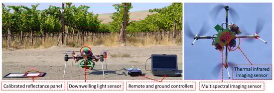
Figure 2.
Unmanned aerial system (UAS) used for multispectral and thermal infrared imaging of grapevines.
2.3. METRIC Implementation
UAS-based imagery was preprocessed as described by Chandel et al. [16], and five surface reflectance, one surface temperature, and one digital elevation model (DEM) orthomosaics were obtained. Figure 3 shows a sample normalized difference vegetation index (NDVI) orthomosaic with irrigation treatments in Block 2.
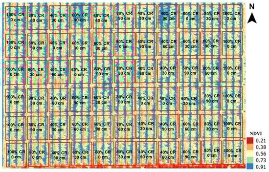
Figure 3.
Small UAS imagery-derived, high-resolution normalized difference vegetation index (NDVI) orthomosaic layer (season: 2019, day before harvest (DBH): 71) showing the surface and direct-root-zone (DRZ) irrigation treatment layout in Block 2.
The implementation of the METRIC model with UAS imagery inputs (UASM approach) was similar to our earlier publication [16], except for momentum roughness length parametrization (Zom, Equation (1), Table 2) described by Carrasco-Benavides et al. [15], Paco et al. [19], Ortega [21], and Perrier [36].
Zom = [(1 − exp(−a × LAI/2) × exp(−a × LAI/2)] × h
a = 2 × f for f ≥ 0.5 and (2 × (1 − f)) − 1 for f < 0.5
Table 2.
Summary of small UAS and conventional Landsat 7/8 imagery-based METRIC model parameters used for grapevine ET estimation.
In Equation (1), the leaf area index (LAI) was estimated using a background adjustment factor (L) of 0.5 in the soil-adjusted vegetation index (SAVI) (Table 2, [37,38,39]). The mean vine height (h) was assumed constant as 2 m. The variability in height was neglected (i) as it resulted in only 3–10% of the variation in Zom, a maximum of 3% in sensible heat flux (H), and 2–3% in the daily ET [15] and (ii) to avoid excessive measurement needs from the grower perspective. Factor f was estimated as the proportion of the LAI above half of the tree height. In the case of vines, f was 1 (a = 2) as nearly the entire canopy foliage exists above 1 m AGL [29,30,40]. Zom was forced to 0.005 m for bare soil surfaces captured at high spatial resolution (7 cm/pixel).
The hot and cold anchor pixels for the METRIC model calibration were selected automatically. Surfaces at the highest temperature, having a low NDVI (<0.3) and Zom (≤0.005 m), were the hot anchors (bare soil). Well-irrigated surfaces at the lowest temperatures with a high NDVI (>0.85), LAI (2.5–6), and Zom (0.03–0.08 m) were the cold pixels. The ET for a cold anchor pixel is assumed to be 1.05 times the ETr (alfalfa-based), with an upper limit of 1.1 for at least 1% of the vegetation within the orthomosaiced imagery that will be healthy and well irrigated throughout the growing season [12,13,14]. The energy-balance-derived instantaneous ET (ETinst, mm h−1) was extrapolated using the 24 h reference ET (ETr24, [12,16]) to obtain the daily ET (mm day−1). Key modified parameters for UASM are summarized in Table 2. UASM was implemented in R (RStudio, Inc., Boston, MA, USA), with the water package as a reference [41].
Additionally, the soil background was segmented in the UASM-ET maps to obtain grapevine canopy transpiration (T) maps. Using the histogram-based segmentation technique, an NDVI of <0.4 was considered as soil background. The resultant UASM-T was compared with the T calculated from the conventional basal crop coefficient (Kcb) approach (FAO 56 [9]), as detailed in Section 2.4.
The Landsat 7/8 cloud-free imagery was also processed using the conventional METRIC model to derive ET maps of the vineyard ([41,42], Table 2), hereafter referred to as the Landsat-METRIC (LM) approach. Surface reflectance products were downloaded for Landsat 8 (source: https://earthexplorer.usgs.gov/ (accessed on 7 April 2020)), while such products for Landsat 7 datasets were calculated within the water package [41].
2.4. Soil-Water-Balance- and Grapevine Basal-Crop-Coefficient-Derived Evapotranspiration
For ET estimation using the SWB approach (Equation (2)), soil moisture data from probes (Sentek Drill & Drop probes, Sacramento, CA, USA; precision: ±0.03%) installed at five locations within Block 2 were used as inputs. Probes were down to 200 cm depth with sensing elements at 20, 40, 60, 80, 100, 140, 160, and 200 cm. Measurements (mm) were logged at 30 min interval, and ET was calculated for a 24 h period on the imaging day. The soil moisture sensor probes were calibrated for local soil conditions using the procedure detailed by the manufacturer.
where, I and P refer to irrigation and precipitation, respectively, that were zero for the imaging days. Dp is the deep percolation, R is the runoff, and Cr is the capillary rise from groundwater that were assumed negligible for drip-irrigated vines. Si and Sf are the soil moisture content at the start and end of the calculation period, respectively.
ET = I + P + Si − Sf − Dp − R + Cr
Tabulated short-grass-based Kcb values (Kcb vine,grass) for three growth stages of wine grapes in arid and semi-arid climates were selected, adjusted as per local conditions, and converted to alfalfa-based Kcb values (Kcb vine,alfalfa, [9], Equations (3)–(6)). These Kcb values were then used to construct seasonal Kcb curves through linear interpolation for the 2018 and 2019 seasons, and T on imaging days was calculated using such curves and pertinent 24 h reference ET (ETr24). ETr24 was calculated using weather data and the Penman–Monteith equation parameterized for an alfalfa reference crop [9].
where u2 is the mean daily wind speed (m s−1), RHmin is the mean daily minimum relative humidity (%) at the pertinent growth stage, Kratio is the ratio for converting the grass-based crop coefficient (Kcb vine,grass) to the alfalfa-based crop coefficient (Kcb vine,alfalfa), and h is the mean vine height (2 m).
Kcb vine(ini/mid/end),grass = Kcb vine (Tab: ini/mid/end),grass + [0.04 × (u2 − 2) − 0.004 × (RHmin − 45)] × (h/3)0.3
Kratio = 1.2 + [0.04 × (u2 − 2) − 0.004 × (RHmin − 45)] × (0.5/3)0.3
Kcb vine,alfalfa = Kcb vine,grass/Kratio
T = Kcb vine,alfalfa × ETr24
2.5. Water Use Analysis
UASM-ET estimates were first compared against SWB-calculated ET estimates. Regions of interest (ROIs) were selected over the five grapevines installed with soil moisture probes, and root-mean-square difference (RMSD) and Pearson’s linear correlation (r) between ET were assessed. UASM-ET estimates were compared with LM-ET estimates. The ET map from the LM approach (36 pixels of 30 × 30 m size each) was clipped to the same area (~3.25 ha) as UASM. The UASM-ET map was then resampled to the LM-ET map (36 pixels). For each campaign, 12 ROIs (30 × 30 m size) were randomly selected in both maps and normalized RMSD (RMSDN, Equation (7)), r, and normalized absolute departures of the mean ET (ETd,MAN, Equation (8)) were assessed between ET estimates. Coefficients of variation (CV, %) were also accessed to compare the spatial water use assessment potentials of UASM and LM approaches.
where i is the pixel number (0–12) and N is the total number of pixels (12).
RMSDN (%) = (∑(ETUASM,I − ETLM,i)2/N)0.5 × 100/Mean(ETLM)
ETd,MAN (%) = |ETUASM − ETLM/FAO-Kcb| × 100/ETLM/FAO-Kcb
Mean T estimates from UASM-T maps were compared to the pertinent T calculated by the FAO-Kcb approach using r and normalized absolute departures of the mean (Td,MAN). For water use (or T) variation assessments due to irrigation treatments, ROIs (100 × 200 cm size) were drawn on the segmented UASM-T map on three central vines in the middle row of each treatment (discussed in Section 2.1). Two-way ANOVAs were then formulated to observe the effects of irrigation rates, DRZ depths, and their interaction on the grapevine T. The mean Kcb for grapevines under all four irrigation rates (100%, 80%, 60%, and 40% of the CR) was estimated from UASM-T maps (TrF, i.e., reference T fraction from T and ETr24) for the same ROIs. Linear interpolated Kcb curves were established and multiplied to the daily ETr to estimate the total water use under each treatment. Total water uses during the treatment period were also calculated using the SWB approach (Equation (2)) and used as a reference to UASM water use estimates. All analyses were conducted at 5% significance (RStudio, Inc., Boston, MA, USA).
3. Results
3.1. Evapotranspiration and Transpiration Mapping
3.1.1. UASM and LM Approaches
For the 2018 season, mean UASM-ET estimates (Figure 4a) ranged from 2.11 to 3.48 mm day−1, while those from the LM approach (Figure 4b) ranged from 1.77 to 3.34 mm day−1. For the 2019 season, such estimates from respective approaches were in the ranges of 2.56–4.08, and 3.61–4.61 mm day−1, respectively. The mean daily ET from the UASM approach was 0.31 mm day−1 (ETd,MAN = 4.29%) less than that from the LM approach, and the mean RMSD for two years did not exceed 0.76 mm day−1 (<22%). Strong and significant correlations (r = 0.70–0.81, Figure 5) were also observed between the UASM and LM-ET estimates. As shown in Figure 4, the GSD plays a key role in UASM capturing high spatial variations (CV = 68 ± 6.67%, (mean ± std. dev.)) compared to the LM (11.85 ± 1.77%) approach (two-sample t-test, t-stat = 20.50, p < 0.001).
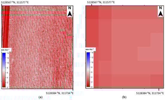
Figure 4.
Sample daily ET maps from (a) UASM and (b) LM approaches for grapevines irrigated at the commercial rate (day of the year: 207, season: 2018).
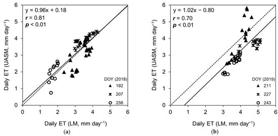
Figure 5.
Comparison plots between daily ET estimates from UASM and LM approaches for grapevines irrigated at the commercial rate on selected days for the (a) 2018 and (b) 2019 growing seasons. DOY: day of the year.
3.1.2. UASM and SWB Approaches
UASM-derived daily ET estimates (2.70 ± 1.03 mm day−1) were significantly higher (two-sample t-test, t-stat = −4.14, p < 0.001) than the ET calculated by the SWB approach (1.80 ± 0.98 mm day−1). However, ET estimates were strongly correlated (r = 0.64–0.81, p < 0.01, Figure 6) with each other in both seasons.
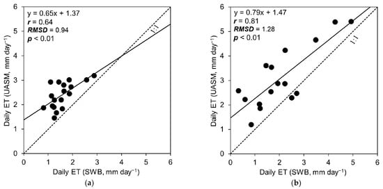
Figure 6.
Comparison between daily ET estimates from UASM and SWB approaches on imaging days for the (a) 2018 and (b) 2019 growing seasons.
3.1.3. UASM and Basal Crop-Coefficient (FAO-Kcb) Approaches
In comparison to the standard FAO-Kcb approach that estimated T in the range of 1.97–5.24 mm day−1 (4 ± 1.54), UASM-T maps derived the mean T in the range of 2.58–5.86 mm day−1 (4.49 ± 1.44). The differences were statistically not significant (two-sample t-test, t-stat = 0.63, p = 0.54). Transpiration trends from both approaches were also strongly correlated (r = 0.95, p < 0.001, Table 3). The UASM approach slightly overestimated T compared to the FAO-Kcb approach (ETd,MAN = ~14%) and was able to estimate spatial water use variability (CV = 29–45%) unlike the FAO-Kcb approach.
Table 3.
Daily transpiration (T) estimates from UASM and FAO-Kcb approaches on the days of flight for grapevines irrigated at the commercial rate.
3.2. Effect of DRZ Irrigation Treatments
The UASM-T maps showed a significant effect of irrigation rates on grapevine water use, as quantified by T for both seasons (two-way ANOVA, F-stat = 7.38–7.78, p < 0.001). However, the DRZ irrigation depth or its interaction with irrigation rates did not have significant effects on water use estimates (p > 0.05). Moreover, no effects were observed at the start of irrigation treatments (DBH: 99 (2018) and DBH: 78 (2019)). For all other imaging campaigns, the mean T of grapevines irrigated at 100% or 80% of the CR was highest, followed by that of grapevines irrigated at 60% and 40% of the CR (Figure 7). The treatment effect was also insignificant on the 10th DBH of the 2019 season, possibly due to a recent irrigation activity (11 DBH).
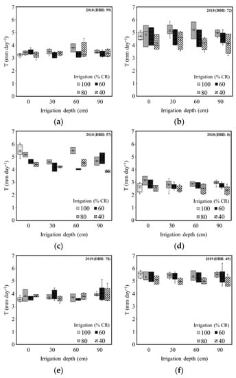
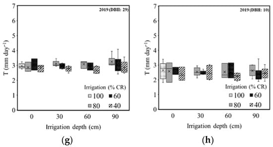
Figure 7.
Daily UASM-T for DRZ-irrigated grapevines at different rate and depth treatments on selected days in the 2018 (a–d) and 2019 (e–h) growing seasons. DBH: days before harvest.
3.3. Seasonal Water Use
Basal crop coefficients (Kcb or TrF) estimated from UASM-T maps for the treatment periods not only followed similar trends as the standard interpolated Kcb curve (FAO approach, non-water-stressed) but also showed high spatiotemporal effects of irrigation rates and canopy growth (Figure 8). Higher magnitudes and temporally advanced trends were observed for the 2019 season (Figure 8b). The grapevine TrF (or Kcb from UASM-T maps) differences for different irrigation rates were non-significant but were notable (Figure 8).
Figure 8.
Basal crop coefficient curves derived from UASM-T maps (non-dotted lines) for grapevines irrigated at different rates in the (a) 2018, and (b) 2019 growth seasons (Ts: treatment start day; S represents locally adjusted standard basal crop coefficient curve pertinent to non-stressed canopy; 40%, 60%, and 80% of the CR were DRZ, and 100% of the CR was surface drip irrigation).
Total water use estimates of grapevines from UASM-T maps for the experimental treatment period were higher compared to the actual amount of water applied for both seasons, but within the range of 5–11% of the actual water use calculated by the SWB approach (Figure 9). Water use was highest for grapevines irrigated at the CR, followed by those irrigated at 80%, 60%, and 40% of the CR. These trends were similar to the amounts of water applied, but they did not decrease in similar proportions. The amounts of applied water and estimated water uses were comparatively lower for the 2019 season for the shorter treatment period (82 days) and low cumulative ETr (Table 1 and Figure 9).
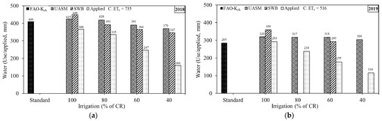
Figure 9.
Crop water use (or total T) and actual water applied during treatments in the (a) 2018 and (b) 2019 growing seasons (C. ETr: cumulative ETr for the treatment period).
4. Discussion
A high CV in the UASM-ET maps (~68%) reflects the potential to geospatially map crop water use variations in an entire vineyard block unlike point measurements (e.g., soil moisture probe, sap flow, and lysimeters) or larger-area estimates (e.g., eddy covariance, crop coefficient approaches). UASM-ET and LM-ET were mostly similar on the days of flight, and a higher ETd,MAN (ET departure) of 16.80% (LM-ET > UASM-ET) was observed for a flight day in the 2019 season. Such differences could be due to variation in the sensible heat flux computation as a result of surface temperatures captured by two imaging platforms and internal model calibrations. Landsat imagery has a coarser resolution (30 × 30 m), with temperatures representing canopy and soil mixes due to large inter-row distances in the vineyards and also restricting identification of uniform anchor pixels near the study area, unlike small UAS imagery [16,43]. A similar mean ET estimation suggests that Zom parameterization did not affect ET computations for bias compensation features of METRIC, as also observed by [15,23].
UASM-T maps estimated a similar mean T as from the FAO-Kcb approach, but the latter does not provide information useful for precision irrigation management. UASM-T maps were able to quantify the effect of DRZ irrigation during the treatment periods of two years. Grapevines irrigated at 100% or 80% of the CR transpired more than those irrigated at 60% and 40% of the CR. In recent studies in the same vineyard block, leaf water potentials [19] and stomatal conductance [32] have been reported to show significant effects of irrigation rates. In some cases, a slightly lower T was estimated for grapevines under 100% of the CR than 80% of the CR, probably because 100% of the CR was surface irrigation at a higher rate that could have contributed to higher evaporation. The non-significant effect of DRZ depths on transpiration estimates could be because DRZ-irrigated grapevines tend to grow their roots near the point of water delivery or water stored in other soil layers to fulfill their evaporative demand [29,34,44,45,46,47].
Trends of UASM-TrF for all treatments were similar as the standard Kcb curve showing variations within 0.3 to 0.8 for the Cabernet Sauvignon cultivar grown in the eastern Washington State [48]. However, notable differences were evident due to the DRZ irrigation rates. Trends of Kcb from UASM-T maps were delayed than the standard curve for the 2019 season most probably due to a cooler temperature in early growth stages (Table 1), delayed canopy growth, and higher preseason snowpack, leading to high soil moisture (Figure 1) [49,50]. Such observations (Figure 8) suggest that FAO-Kcb can be off the mark if standard phenology periods are used, which differ from actual field phenology that does not affect UASM. Furthermore, UASM assesses spatial water use to potentially aid site-specific management, unlike FAO-Kcb that calculates a single value for an entire area and is restricted to seasonal water application management [51,52].
Cumulative water use estimated from UASM approach was within 5–11% of the SWB-based water use calculations. Overall, water usage for grapevines under different irrigation rates did not decrease as the actual amount of applied water. These differences may be possibly due to the water utilization from non-irrigated zones [45,46,47,53,54,55]. The non-irrigated zones could store water in deeper or lateral soil layers from precipitation and snowpack of the previous growing season until initiation of irrigation treatments in the current season. Such supplemented water usage was higher in the 2018 season due to higher evaporative demand compared to the 2019 season. Pertinent water uptake by grapevines would have minimized the differences between deficit irrigation (80%, 60%, and 40% of the CR) and those under 100% of the CR. The lower the amount of water applied, the more was the compensation from stored water until all of that was exhausted. Higher UASM-estimated transpiration compared to SWB estimates for deficit-irrigated grapevines could most probably be due to additional water use from lateral soil zones, as reflected in UASM but outside the volume sensed by the moisture probes. For the surface-drip-irrigated grapevines at 100% of the CR, the UASM-estimated transpiration was lower compared to SWB estimates. This could be due to higher water evaporation from soil surface in those treatments [56].
The study site typically receives high preseason snowpack. The site comprises sandy soil at the surface and highly stratified, silty soil layers beyond a 1 m depth [35]. Since the water-holding capacity is very high for silty soil, the melted snow water could have been stored in those deep silt layers that would be potentially available for use during the growth season. This enhances the chances of deficit-irrigated grapevines to maintain their Kcb in healthy ranges using supplementary water stored in other soil layers through deeper or lateral roots. Such root behavior was also observed by Bauerle et al. [57] for Merlot grapevines, where drought-resistant varieties had higher root production in deeper soil layers during summer. A similar study by Soar and Loveys [58] on Cabernet Sauvignon reported that the vines converted from an under-sprinkler to a drip irrigation system had significantly larger root systems compared to those under constant sprinkler irrigation. Deeper and lateral root development was also observed in related studies on the experimental site [30,34] used in this study. These studies reported that DRZ-irrigated grapevines had 80% roots down to a 160 cm depth, and the remaining 20% roots were much deeper in the soil profile. For the surface irrigation treatments, almost all the roots were accumulated in the top 60 cm of the soil. Such root growth under DRZ treatments would use stored water from other soil layers for uncompromised photosynthesis rates and yield.
5. Conclusions
UAS imagery was successfully used with the METRIC model (UASM) to map spatiotemporal water use for two growth seasons of a surface and sub-surface drip-irrigated vineyard. For days of Landsat overpass, the UASM approach estimated higher but comparable ET as the SWB approach (r = 0.64–0.81, p < 0.01) and conventional LM approach (mean RMSDN = ~22%, mean r = 0.83, ETd,MAN = ~4.30%). UASM also had similar grapevine transpiration estimates as the standard FAO-Kcb approach (r = 0.95, Td,MAN = ~14%, p < 0.01). This supports the suitability of small UAS-based multispectral and thermal imaging for reliably estimating ET and T at high geospatial resolution for heterogeneous crops. Furthermore, a high spatial variation in crop water use could be assessed by the UASM approach (CV = 68 ± 6.67%), which other standard or point measurement approaches could not assess. The high-resolution (GSD: 7 cm/pixel) UASM-T maps could adequately assess crop water use variations of grapevines as an effect of irrigation rates (p < 0.01), where grapevines under 100% or 80% of the CR transpired consistently higher than those irrigated at 60% and 40% of the CR. UASM-estimated basal crop coefficients (TrF or Kcb) also reflected the effects of deficit irrigation treatments. Using those crop coefficients, UASM estimated the total crop water use for grapevines under surface and DRZ treatments, unlike the proportions of the actual amount of applied water. With such observations, the UASM approach highlighted the phenomena reported in other studies that deficit-irrigated grapevines might be fulfilling their evaporative demand from water stored in other soil layers through deeper or laterally developed roots. Overall, study findings indicate that UAS-based high-resolution imagery may be useful for site-specific spatial irrigation management of grapevines and other perennial specialty crops.
Author Contributions
Conceptualization, A.K.C., L.R.K., C.O.S., R.T.P., and B.M.; data curation, A.K.C., L.R.K., and B.M.; funding acquisition, L.R.K., R.T.P., and C.O.S.; drone flights, A.K.C. and B.M.; investigation, A.K.C. and B.M.; methodology, A.K.C., L.R.K., and C.O.S.; project administration, L.R.K., R.T.P., and C.O.S.; resources, L.R.K., R.T.P., C.O.S., and P.W.J.; software, A.K.C. and L.R.K.; supervision, L.R.K., R.T.P., and C.O.S.; validation, A.K.C. and B.M.; visualization, A.K.C., B.M., L.R.K., R.T.P., and C.O.S.; writing—original draft, A.K.C.; writing—review and editing, A.K.C., L.R.K., B.M., R.T.P., C.O.S., and P.W.J. All authors have read and agreed to the published version of the manuscript.
Funding
This research was funded, in part, by the United States Department of Agriculture—National Institute of Food and Agriculture projects 1016467, WNP0745, and WNP0839 and the Washington State University—CAHNRS Office of Research Emerging Research Issues Internal Competitive Grant Program.
Acknowledgments
We thank the grower cooperator Scott Williams, the general manager of Kiona Vineyards and Winery near Benton City, Washington, DC, USA.
Conflicts of Interest
The authors declare no conflict of interest.
References
- McCarthy, M.G. Developmental variation in sensitivity of Vitis vinifera L. (Shiraz) berries to soil water deficit. Aust. J. Grape Wine Res. 2000, 6, 136–140. [Google Scholar] [CrossRef]
- Santesteban, L.G.; Miranda, C.; Royo, J.B. Regulated deficit irrigation effects on growth, yield, grape quality and individual anthocyanin composition in Vitis vinifera L. cv. ‘Tempranillo’. Agric. Water Manag. 2011, 98, 1171–1179. [Google Scholar] [CrossRef]
- Styles, J.; Stevens, R.; Grigson, G.; Ewenz, C.; Williams, C. Seasonal Variation of Crop Water Use, Soil Water Balance and Vine Transpiration in a Riverland Vineyard. SARDI Publication Number F2009/000000-1; South Australian Research and Development Institute: Urrbrae, Australia, 2015. [Google Scholar]
- Yunusa, I.A.M.; Walker, R.R.; Lu, P. Evapotranspiration components from energy balance, sap flow and microlysimetry techniques for an irrigated vineyard in inland Australia. Agric. For. Meteorol. 2004, 127, 93–107. [Google Scholar] [CrossRef]
- Ferreira, M.I.; Silvestre, J.; Conceição, N.; Malheiro, C.A. Crop and stress coefficients in rainfed and deficit irrigation vineyards using sap flow techniques. Irrig. Sci. 2012, 30, 433–447. [Google Scholar] [CrossRef]
- Fooladmand, H.R.; Sepaskhah, A.R. A soil water balance model for a rain-fed vineyard in a micro catchment based on dual crop coefficient. Arch. Agron. Soil Sci. 2009, 55, 67–77. [Google Scholar] [CrossRef]
- Ortega-Farias, S.; Poblete-Echeverria, C.; Brisson, N. Parameterization of a two-layer model for estimating vineyard evapotranspiration using meteorological measurements. Agric. For. Meteorol. 2010, 150, 276–286. [Google Scholar] [CrossRef]
- Rodríguez, J.C.; Grageda, J.; Watts, C.J.; Garatuza-Payan, J.; Castellanos-Villegas, A.; Rodríguez-Casas, J.; Saiz-Hernández, J.; Olavarrieta, V. Water use by perennial crops in the lower Sonora watershed. J. Arid Environ. 2010, 74, 603–610. [Google Scholar] [CrossRef]
- Allen, R.G.; Pereira, L.S.; Raes, D.; Smith, M. FAO Irrigation and Drainage Paper No. 56; Food and Agriculture Organization of the United Nations: Rome, Italy, 1998; Volume 56, p. e156. [Google Scholar]
- Phogat, V.; Skewes, M.A.; McCarthy, M.G.; Cox, J.W.; Šimůnek, J.; Petrie, P.R. Evaluation of crop coefficients, water productivity, and water balance components for wine grapes irrigated at different deficit levels by a sub-surface drip. Agric. Water Manag. 2017, 180, 22–34. [Google Scholar] [CrossRef]
- McShane, R.R.; Driscoll, K.P.; Sando, R. A Review of Surface Energy Balance Models for Estimating Actual Evapotranspiration with Remote Sensing at High Spatiotemporal Resolution over Large Extents. In Scientific Investigations Report 2017; U.S. Department of the Interior, U.S. Geological Survey: Reston, VA, USA, 2017. [Google Scholar]
- Allen, R.G.; Tasumi, M.; Trezza, R. Satellite-based energy balance for mapping evapotranspiration with internalized calibration (METRIC)-Model. J. Irrig. Drain. Eng. 2007, 133, 380–394. [Google Scholar] [CrossRef]
- Allen, R.G.; Tasumi, M.; Morse, A.; Trezza, R.; Wright, J.L.; Bastiaanssen, W.; Kramber, W.; Lorite, I.J.; Robison, C.W. Satellite-based energy balance for mapping evapotranspiration with internalized calibration (METRIC)—Applications. J. Irrig. Drain. Eng. 2007, 133, 395–406. [Google Scholar] [CrossRef]
- Allen, R.; Irmak, A.; Trezza, R.; Hendrickx, J.M.; Bastiaanssen, W.; Kjaersgaard, J. Satellite-based ET estimation in agriculture using SEBAL and METRIC. Hydrol. Process. 2011, 25, 4011–4027. [Google Scholar] [CrossRef]
- Carrasco-Benavides, M.; Ortega-Farías, S.; Lagos, L.; Kleissl, J.; Morales-Salinas, L.; Kilic, A. Parameterization of the satellite-based model (METRIC) for the estimation of instantaneous surface energy balance components over a drip-irrigated vineyard. Remote Sens. 2014, 6, 11342–11371. [Google Scholar] [CrossRef]
- Chandel, A.K.; Molaei, B.; Khot, L.R.; Peters, R.T.; Stöckle, C.O. Small UAS-based multispectral and thermal infrared imagery driven energy balance model for high-resolution evapotranspiration estimation of irrigated field crops. Drones 2020, 4, 52. [Google Scholar] [CrossRef]
- Chávez, J.L.; Torres-Rua, A.; Boldt, W.E.; Zhang, H.; Robertson, C.; Marek, G.; Wang, D.; Heeren, D.; Taghvaeian, S.; Neale, C.M. A Decade of Unmanned Aerial Systems in Irrigated Agriculture in the Western US. Appl. Eng. Agric. 2020, 36, 423–436. [Google Scholar] [CrossRef]
- Santos, C.; Lorite, I.J.; Allen, R.G.; Tasumi, M. Aerodynamic Parameterization of the Satellite-Based Energy Balance (METRIC) Model for ET Estimation in Rainfed Olive Orchards of Andalusia, Spain. Water Resour. Manag. 2012, 26, 3267–3283. [Google Scholar] [CrossRef]
- Paço, T.A.; Pôças, I.; Cunha, M.; Silvestre, J.C.; Santos, F.L.; Paredes, P.; Pereira, L.S. Evapotranspiration and crop coefficients for a super intensive olive orchard. An application of SIMDualKc and METRIC models using ground and satellite observations. J. Hydrol. 2014, 519, 2067–2080. [Google Scholar] [CrossRef]
- Pôças, I.; Paço, T.A.; Cunha, M.; Andrade, J.A.; Silvestre, J.; Sousa, A.; Santos, F.L.; Pereira, L.S.; Allen, R.G. Satellite-based evapotranspiration of a super-intensive olive orchard: Application of METRIC algorithms. Biosyst. Eng. 2014, 128, 69–81. [Google Scholar] [CrossRef]
- Ortega, S. EVALUATION of the METRIC Model for Mapping Energy Balance Components and Actual Evapotranspiration for a Super-Intensive Drip-Irrigated Olive Orchard. Ph.D. Thesis, University of Nebraska-Lincoln, Lincoln, NE, USA, 2019. [Google Scholar]
- la Fuente-Sáiz, D.; Ortega-Farías, S.; Fonseca, D.; Ortega-Salazar, S.; Kilic, A.; Allen, R. Calibration of metric model to estimate energy balance over a drip-irrigated apple orchard. Remote Sens. 2017, 9, 670. [Google Scholar] [CrossRef]
- Carrasco-Benavides, M.; Ortega-Farías, S.; Lagos, L.O.; Kleissl, J.; Morales, L.; Poblete-Echeverría, C.; Allen, R.G. Crop coefficients and actual evapotranspiration of a drip-irrigated Merlot vineyard using multispectral satellite images. Irrig. Sci. 2012, 30, 485–497. [Google Scholar] [CrossRef]
- Cammalleri, C.; Anderson, M.C.; Gao, F.; Hain, C.R.; Kustas, W.P. A data fusion approach for mapping daily evapotranspiration at field scale. Water Resour. Res. 2013, 49, 4672–4686. [Google Scholar] [CrossRef]
- Zipper, S.C.; Loheide II, S.P. Using evapotranspiration to assess drought sensitivity on a subfield scale with HRMET, a high-resolution surface energy balance model. Agric. For. Meteorol. 2014, 197, 91–102. [Google Scholar] [CrossRef]
- Xia, T.; Kustas, W.P.; Anderson, M.C.; Alfieri, J.G.; Gao, F.; McKee, L.; Prueger, J.H.; Geli, H.M.; Neale, C.M.; Sanchez, L.; et al. Mapping evapotranspiration with high-resolution aircraft imagery over vineyards using one-and two-source modeling schemes. Hydrol. Earth Syst. Sci. 2016, 20, 1523–1545. [Google Scholar] [CrossRef]
- Fandino, M.; Cancela, J.J.; Rey, B.J.; Martinez, E.M.; Rosa, R.G.; Pereira, L.S. Using the dual-Kc approach to model evapotranspiration of Albarino vineyards (Vitis vinifera L cv. Albarino) with consideration of active ground cover. Agric. Water Manag. 2012, 112, 75–87. [Google Scholar] [CrossRef]
- Cancela, J.J.; Fandino, M.; Rey, B.J.; Martínez, E.M. Automatic irrigation system based on dual crop coefficient, soil and plant water status for Vitis vinifera (cv Godello and cv Mencía). Agric. Water Manag. 2015, 151, 52–63. [Google Scholar] [CrossRef]
- Ma, X.; Sanguinet, K.A.; Jacoby, P.W. Performance of direct root-zone deficit irrigation on Vitis vinifera L. cv. Cabernet Sauvignon production and water use efficiency in semi-arid southcentral Washington. Agric. Water Manag. 2019, 221, 47–57. [Google Scholar] [CrossRef]
- Ma, X.; Sanguinet, K.A.; Jacoby, P.W. Direct root-zone irrigation outperforms surface drip irrigation for grape yield and crop water use efficiency while restricting root growth. Agric. Water Manag. 2020, 231, 105993. [Google Scholar] [CrossRef]
- Baluja, J.; Diago, M.P.; Balda, P.; Zorer, R.; Meggio, F.; Morales, F.; Tardaguila, J. Assessment of vineyard water status variability by thermal and multispectral imagery using an unmanned aerial vehicle (UAV). Irrig. Sci. 2012, 30, 511–522. [Google Scholar] [CrossRef]
- Espinoza, C.Z.; Khot, L.R.; Sankaran, S.; Jacoby, P.W. High resolution multispectral and thermal remote sensing-based water stress assessment in subsurface irrigated grapevines. Remote Sens. 2017, 9, 961. [Google Scholar] [CrossRef]
- Chávez, J.L.; Gowda, P.H.; Howell, T.A.; Garcia, L.A.; Copeland, K.S.; Neale, C.M.U. ET mapping with high-resolution airborne remote sensing data in an advective semiarid environment. J. Irrig. Drain. Eng. 2012, 138, 416–423. [Google Scholar] [CrossRef]
- Ma, X.; Jacoby, P.W.; Sanguinet, K.A. Improving Net Photosynthetic Rate and Rooting Depth of Grapevines Through a Novel Irrigation Strategy in a Semi-Arid Climate. Front. Plant Sci. 2020, 11, 575303. [Google Scholar]
- Busacca, A.J.; Norman, D.K.; Wolfe, W. Geologic Guide to the Yakima Valley Wine-Growing Region, Benton and Yakima Counties, Washington; Washington State Department of Natural Resources: Washington, DC, USA, 2008.
- Perrier, A. Land surface processes: Vegetation. In Land Surface Processes in Atmospheric General Circulation Models; Eagleson, P.S., Ed.; Cambridge University Press: Cambridge, UK, 1982; pp. 395–448. [Google Scholar]
- Candiago, S.; Remondino, F.; De Giglio, M.; Dubbini, M.; Gattelli, M. Evaluating Multispectral Images and Vegetation Indices for Precision Farming Applications from UAV Images. Remote Sens. 2015, 7, 4026–4047. [Google Scholar] [CrossRef]
- Aboutalebi, M.; Torres-Rua, A.F.; McKee, M.; Kustas, W.; Nieto, H.; Coopmans, C. Behavior of vegetation/soil indices in shaded and sunlit pixels and evaluation of different shadow compensation methods using UAV high-resolution imagery over vineyards. In Autonomous Air and Ground Sensing Systems for Agricultural Optimization and Phenotyping III; International Society for Optics and Photonics: Orlando, Florida, USA, 2018; Volume 10664, p. 1066407. [Google Scholar]
- Jorge, J.; Vallbe, M.; Soler, J.A. Detection of irrigation in homogeneities in an olive grove using the NDRE vegetation index obtained from UAV images. Eur. J. Remote Sens. 2019, 52, 169–177. [Google Scholar] [CrossRef]
- Espinoza, C.Z.; Rathnayake, A.P.; Chakraborty, M.; Sankaran, S.; Jacoby, P.W.; Khot, L.R. Applicability of time-of-flight-based ground and multispectral aerial imaging for grapevine canopy vigour monitoring under direct root-zone deficit irrigation. Int. J. Remote Sens. 2018, 39, 8818–8836. [Google Scholar] [CrossRef]
- Olmedo, G.F.; Ortega-Farías, S.; de la Fuente-Sáiz, D.; Fonseca-Luego, D.; Fuentes-Peñailillo, F. Water: Tools and Functions to Estimate Actual Evapotranspiration Using Land Surface Energy Balance Models in R. R. J. 2016, 8, 352–369. [Google Scholar] [CrossRef]
- Jaafar, H.H.; Ahmad, F.A. Time series trends of Landsat-based ET using automated calibration in METRIC and SEBAL: The Bekaa Valley, Lebanon. Remote Sens. Environ. 2020, 238, 111034. [Google Scholar] [CrossRef]
- Elarab, M. The Application of Unmanned Aerial Vehicle to Precision Agriculture: Chlorophyll, Nitrogen, and Evapotranspiration Estimation. Ph.D. Thesis, Utah State University, Logan, UT, USA, 2016. [Google Scholar]
- van Leeuwen, C.; Friant, P.; Choné, X.; Tregoat, O.; Koundouras, S.; Dubourdieu, D. Influence of climate, soil, and cultivar on terroir. Am. J. Enol. Vitic. 2004, 55, 207–217. [Google Scholar]
- Grigg, D.; Methven, D.; de Bei, R.; Rodríguez López, C.M.; Dry, P.; Collins, C. Effect of vine age on vine performance of Shiraz in the Barossa Valley, Australia. Aust. J. Grape Wine Res. 2018, 24, 75–87. [Google Scholar] [CrossRef]
- Nader, K.B.; Stoll, M.; Rauhut, D.; Patz, C.D.; Jung, R.; Loehnertz, O.; Schultz, H.R.; Hilbert, G.; Renaud, C.; Roby, J.P.; et al. Impact of grapevine age on water status and productivity of Vitis vinifera L. cv. Riesling. Eur. J. Agron. 2019, 104, 1–12. [Google Scholar] [CrossRef]
- Scholasch, T.; Rienth, M. Review of water deficit mediated changes in vine and berry physiology; Consequences for the optimization of irrigation strategies. OENO One 2019, 53. [Google Scholar] [CrossRef]
- Moyer, M.; Mills, L.J. Grapevine Crop Coefficient (Kc); Washington State University Extension: Washington, DC, USA, 2017. [Google Scholar]
- Pearce, I.; Coombe, B.G. Grapevine phenology. In Viticulture Volume 1—Resources, 2nd ed.; Dry, P.R., Coombe, B.G., Eds.; Winetitles: Adelaide, Australia, 2005; pp. 150–166. [Google Scholar]
- Chalmers, Y. Insights into the relationships between yield and water in wine grapes. In Grape and Wine Research and Development Corporation; Department of Agriculture, Fisheries and Forestry of the Government of Australia: Canberra, Australia, 2012. [Google Scholar]
- Poblete-Echeverría, C.A.; Ortega-Farias, S.O. Evaluation of single and dual crop coefficients over a drip-irrigated M erlot vineyard (Vitis vinifera L.) using combined measurements of sap flow sensors and an eddy covariance system. Aust. J. Grape Wine Res. 2013, 19, 249–260. [Google Scholar] [CrossRef]
- Vanino, S.; Pulighe, G.; Nino, P.; De Michele, C.; Bolognesi, S.F.; D’Urso, G. Estimation of evapotranspiration and crop coefficients of tendone vineyards using multi-sensor remote sensing data in a mediterranean environment. Remote Sens. 2015, 7, 14708–14730. [Google Scholar] [CrossRef]
- Dry, P.R.; Loveys, B.R.; During, H. Partial drying of the rootzone of grape. II. Changes in the pattern of root development. Vitis 2000, 39, 9–12. [Google Scholar]
- Kriedemann, P.E.; Goodwin, I. Regulated Deficit Irrigation and Partial Rootzone Drying; Land & Water: Canberra, Australia, 2003. [Google Scholar]
- Munitz, S.; Netzer, Y.; Schwartz, A. Sustained and regulated deficit irrigation of field-grown Merlot grapevines. Aust. J. Grape Wine Res. 2017, 23, 87–94. [Google Scholar] [CrossRef]
- Evett, S.R.; Colaizzi, P.D.; Howell, T.A. Drip and evaporation. In Proceedings of the 2005 Central Plains Irrigation Conference, Sterling, CO, USA, 16–17 February 2007. [Google Scholar]
- Bauerle, T.L.; Smart, D.R.; Bauerle, W.L.; Stockert, C.; Eissenstat, D.M. Root foraging in response to heterogeneous soil moisture in two grapevines that differ in potential growth rate. New Phytol. 2008, 179, 857–866. [Google Scholar] [CrossRef] [PubMed]
- Soar, C.J.; Loveys, B.R. The effect of changing patterns in soil-moisture availability on grapevine root distribution, and viticultural implications for converting full-cover irrigation into a point-source irrigation system. Aust. J. Grape Wine Res. 2007, 13, 2–13. [Google Scholar] [CrossRef]


Publisher’s Note: MDPI stays neutral with regard to jurisdictional claims in published maps and institutional affiliations. |
© 2021 by the authors. Licensee MDPI, Basel, Switzerland. This article is an open access article distributed under the terms and conditions of the Creative Commons Attribution (CC BY) license (http://creativecommons.org/licenses/by/4.0/).