Abstract
In the frame of an SMOS follow-on operational mission, a new instrument design is being developed based on the lessons learned from MIRAS, the SMOS payload. To reduce hardware complexity and mass, digital In-phase Quadrature (IQ) demodulation is considered. In this schema, Q components are obtained by delaying one clock of the digitized IF signals instead of using phase quadrature analog mixers. The purpose of this article is to formulate this concept for application to interferometric radiometry, establish the required data processing methods, and provide experimental results.
1. Introduction
Interferometric radiometry is a technique to obtain brightness temperature images using large arrays of antennas in order to achieve a spatial resolution similar to that of real apertures of a similar size. It has been used for decades in radio astronomy and has been successfully applied for Earth observation in the ESA’s (European Space Agency) SMOS (Soil Moisture and Ocean Salinity) mission.
SMOS is an eleven-year-old satellite currently providing sea surface salinity, soil moisture, ice sheet cover, ocean winds, and other scientific products on a continuous basis from its launch in 2009 [1,2]. In the frame of developing an SMOS follow-on operational mission, a new instrument design was proposed taking into account the lessons learned [3] from the SMOS single payload MIRAS [4] (Microwave Interferometric Radiometer with Aperture Synthesis). The new instrument includes, for each individual antenna, two independent receiver chains, one for each polarization, to reduce smearing in the horizontal/vertical maps and facilitate the full polarimetric operation. Furthermore, to increase radiometric performances, a hexagonal structure is considered [5], so the total number of receivers becomes larger (74% increase) than its counterpart MIRAS.
In order to reduce hardware complexity and mass while keeping performances, all receivers use digital In-phase Quadrature (IQ) demodulation instead of the classical analog mixers with phase and quadrature local oscillators. A single frequency conversion shifts the Radio Frequency (RF) signal spectrum to an Intermediate Frequency (IF) low enough to allow using standard hardware for analog-to-digital conversion. The quadrature component is obtained by delaying one quarter of a period, equivalent to shifting the phase of the IF signal. The sampling frequency is chosen as four times the center frequency in order to implement the delay just by selecting the previous sample of a given epoch, so greatly simplifying the signal processing. This technique is used in digital communication receivers, and the purpose of this paper is to formulate it for interferometric radiometry taking into account that input signals are Gaussian band-pass processes.
The study is carried out as part of an ESA project for developing two units of the Advanced Receiver for the Future L-Band Radiometer (ALR). Each receiver is composed of two high gain superheterodyne chains operating at a center frequency of 1413.5 MHz and producing one-bit digitized IF outputs, as well as low frequency signals from analog power detectors. The purpose of the project is to serve as a demonstrator of an interferometric radiometer baseline for the SMOS follow-on mission. The receiver and the characterization equipment were designed and manufactured by the Spanish company SENER TAFS S.A.U. in Barcelona.
The paper shows the theoretical formulation and expected performances of the digital IQ demodulation, as well as results from digital correlation measurements and a comparison with theoretical predictions.
2. Materials and Methods
2.1. Visibility and Correlation
Visibility is the fundamental measurement of an interferometric radiometer. It is a complex function of the relative antenna positions linearly related to the brightness temperature of the source through an integral transform [6]. For any baseline formed by two antennas, it is proportional to the complex cross-correlation of the corresponding analytic signals [7,8] representing the thermal noise waves collected by the antennas. If and are the analytic signals out of receivers k and j, respectively, their cross-correlation at zero lag is:
where k is the Boltzmann constant, and respectively the available power gain and noise equivalent bandwidth of the receivers, the correlator complex gain, and the visibility. To be precise and consistent with [6], the visibility function is here normalized with respect to the fringe washing function (see Appendix A) at the origin, equal to the correlator gain . By using this normalization, used also in SMOS processing [9], the integral relation between visibility and brightness temperature only includes the shape of the fringe washing function , which is unity for by definition.
The particular case when both antennas collapse into a single one is the autocorrelation, proportional to the system temperature:
A one-bit, two-level digital correlation, as the one used in MIRAS and considered throughout this paper, measures the normalized cross-correlation:
In an interferometric radiometer such as MIRAS, is measured by a complex correlator, the system temperatures by “Power Measurement Systems” (PMS) included in each receiver, and by internal calibration injecting correlated noise [9,10]. The visibility is then solved from the above equation, and the brightness temperature is finally obtained by inverting the visibility equation [11].
2.2. In-Phase and Quadrature
A correlator is a piece of hardware that multiplies two input voltages (real waveforms) and filters the output. The result is a low frequency signal proportional to the real part of the complex cross-correlation of the corresponding analytic signals (numerator of (3)). The imaginary part is obtained by multiplying one of the the analytic signals by :
or, equivalently in signal theory terms, by correlating one signal with the Hilbert transform of the other. In the frequency domain, this transform is equivalent to applying a 90-degree constant phase shift, so this signal can be said to be in “quadrature” with the original one. In an analog IQ demodulator, such as the one used in MIRAS, this 90-degree phase difference is achieved by using two mixers driven by corresponding local oscillators in quadrature to each other, as shown in the block diagram of the left of Figure 1. Note that differences in the two band-pass filter responses are responsible for the quadrature error, which can be corrected using the algorithms provided in [9].
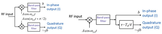
Figure 1.
Two systems of implementing a Hilbert transform, or producing a quadrature signal. Left: An analog IQ mixer. Right: Using a quarter period delay.
The method proposed here is depicted in the block diagram on the right of Figure 1. It uses a time delay equal to a quarter of a period of the center frequency to generate the quadrature output. Of course, the 90-degree shift is only achieved exactly at the center frequency, so the method is only strictly applicable to narrow to moderate band signals. There is no quadrature error, but there is center frequency error and decorrelation. The analog version hardware is much more complex: it needs both Radio Frequency (RF) and Local Oscillator (LO) splitters, a phase shifter, two mixers, and two band-pass filters. Furthermore, there are two output signals to be sent to the correlator, while in the digital version, there is only one since the delay is produced by selecting the previous sample (see Section 2.4). The main purpose of this paper is to propose a digital implementation and also analyze the limitations and error correction techniques of this strategy.
2.3. Normalized Cross-Correlation Function
A time-domain real waveform is, by definition, the real part of its analytic signal. Without loss of generality, this one can be written in terms of the “complex envelope” [7] referenced to an arbitrary frequency . Using this representation, the output waveforms (typically at IF) of two receivers forming a baseline of an interferometric radiometer can be written as:
where are the corresponding complex envelopes and the terms inside the brackets are the analytic signals. The cross-correlation function of the real signals and is readily computed as:
in which it has been taken into account that the term at vanishes. Now, it must be recalled that, by definition, the cross-correlation function is the Fourier transform of the cross-power spectral density. Then, using the methods outlined in the Appendix of [6], the cross-power spectral density of the complex envelopes can be expressed in terms of the visibility and the filters’ response. After some manipulations, (6) can be written as:
where is the fringe washing function (see Appendix A) referenced to and normalized to its value at the origin . It is a function of the frequency domain signal spectra and depends ultimately on the receivers’ frequency responses. Similar equations hold for the autocorrelation functions of each signal, in this case as a function of the system temperatures instead of the visibility. Now, using the definition (3), the normalized cross-correlation function between both time-domain real waveforms becomes:
The following property is a direct consequence of (8):
and for the particular case of a single receiver (for example, unit k), (8) reduces to:
in which the fringe washing function need not be normalized since always . Note that (9) implies that and are even functions of .
As indicated in the block diagram in the right part of Figure 1, the quadrature signal used to get the imaginary part of the visibility is obtained by introducing a delay. In digital systems, this is easily implemented after Analog-to-Digital (A/D) conversion by shifting one or more one-bit samples, so any delay must be a multiple of the sampling period , with the sampling frequency. Furthermore, the delay must be one quarter of a period of the center frequency. Considering a single bit shift, the sampling frequency is then set to four times the nominal center frequency. If this one is also used as the reference frequency of the fringe washing function (see Appendix A), then:
which substituted into (8) yields:
Since the actual receivers’ center frequency may differ from the nominal one , the fringe washing function is in general complex and not-symmetrical around the origin (see Appendix A). In any case, (12) implies that , and neglecting the normalized fringe washing function, , demonstrating that this concept is able to recover both the real and the imaginary parts of the normalized complex correlation and hence of the visibility. In general, due to the time delay, the imaginary part is affected by some degree of decorrelation quantified by the normalized fringe washing function. This one can be important for systems with a large bandwidth, but can be compensated by proper processing, as explained in Section 2.4.1.
2.4. Data Processing
A digital correlator based on this concept measures all correlation products between the I and Q signals defined in the block diagram of the right of Figure 1. Both of them are obtained by sampling the output IF signal at the clock period . At a given epoch, the I signal is just the measured sample, and the Q signal is the one at the previous epoch. According to this schema, Figure 2 provides a representation of the sampling strategy to measure all four correlation products.
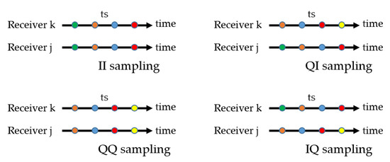
Figure 2.
Sampling strategy to measure the four real correlation products. Each color represents a complete and consistent set for a given snapshot and is the sampling period. Note that, for example, the II measurement of the blue snapshot is the same as the QQ of the red snapshot. In this drawing, green and yellow snapshots are not complete.
Particularizing (12), they can be written as:
and the self-“IQ” correlation of a single receiver (k):
In all above equations, the zero in parenthesis indicates “zero delay” apart from the one used to get the Q signal. Later in Section 2.5, additional delays will be considered. Using now the following definitions:
and defining also the nominal and redundant complex correlations as:
Equations (13)–(15) can be solved for , resulting in:
where the constant M is:
in which the plus sign applies to redundant correlation and the minus sign to nominal. In fact, only one kind of correlation, either nominal or redundant, is needed since both of them provide exactly the same measurement. In summary, provided the fringe washing function at is known, the above equations allow retrieving the corrected complex normalized correlation out of the raw measurements.
2.4.1. Decorrelation of the Imaginary Part
If, according to the property 5 of the fringe washing function (Appendix A), this one is approximated by just a function, then (21) simplifies to , and (20) approximates to:
so the real part of is correctly retrieved, while the imaginary part needs a correction for the decorrelation quantified by the fringe washing function. Substituting for example MHz and MHz, it follows that, for the nominal case, .
Equation (22) can be used to get a first estimation of the corrected normalized correlation directly from the correlation products’ measurements. Note that the constant affecting the imaginary part is only an educated guess based on the approximated shape of the fringe washing function. For narrow band systems with , the denominator of (22) becomes close to one, so the error is small. If the receiver’s bandwidth increases, the denominator decreases, incrementing the retrieval noise. The term becomes singular if , and then, no retrieval is possible.
2.4.2. Center Frequency Error
Consider that the frequency response of a given receiver is centered on , different from the nominal value , so that:
Then, still using the approximation, the fringe washing function of the single receiver k is:
where the property 4 of the fringe washing function was used. Introducing this result into (16), the correlation of adjacent samples becomes:
Note that, if the nominal center frequency coincides with the actual value (), then this correlation vanishes. Otherwise, it can be used to estimate the center frequency as:
in which (11) was used. This operation can be carried out for each individual receiver to obtain its corresponding center frequency, which in general are different from each other.
On the other hand, using the same approximations, the normalized fringe washing function of the baseline becomes identical to that of a single receiver (24) and can be written as:
where is the center frequency error for the baseline, which can be set equal to the average of those estimated from the self-IQ correlation of each receiver (25). The above Equation (27) can be directly introduced into (21) to get the correction factor M for the imaginary part of the correlation:
which in turn is substituted into (20) to obtain the corrected normalized correlation . Without additional information, this is the best correction that can be applied to the raw measurements in order to estimate the corrected normalized correlation .
2.5. Fringe Washing Function Shape
In the MIRAS instrument, the fringe washing function shape is characterized by measuring correlations at three time delays , zero, and [12]. This procedure is neat since at each delay, a complete and consistent set of correlation products is measured. However, in the proposed digital IQ demodulator, some correlation products include already a time delay to retrieve the imaginary part of the complex correlation. To avoid conflict, the three delays must be set to , zero, and .
2.5.1. Three-Delay Measurements
Delay 0 means using directly the sampling strategy depicted in Figure 2. Taking as the reference the red dots in this figure, delaying two clock periods, the signals of either receiver k or j mean using the sampling strategy schematized in Figure 3 and Figure 4, respectively.
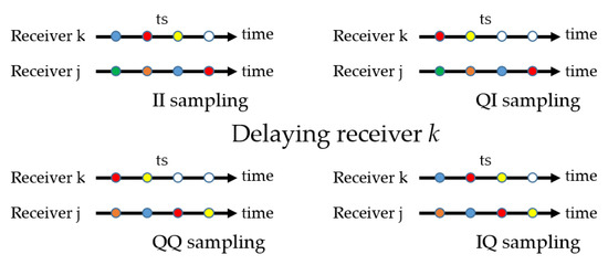
Figure 3.
Sampling strategy for delaying receiver k two clock periods based on the non-delayed reference of Figure 2. Only the red snapshot is complete.
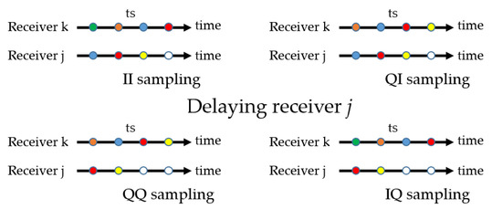
Figure 4.
Sampling strategy for delaying receiver j two clock periods based on the non-delayed reference of Figure 2. Only the red snapshot is complete.
The combination of delaying one clock to measure the IQ or QI product and the additional delay of one or other signals results in different overall delays that must be analyzed with care. For example, the IQ product with receiver k delayed (bottom right of Figure 3) for the red snapshot coincides with the QI product with no delay (top right of Figure 2) for the blue snapshot. The same happens between the product QI with receiver j delayed and IQ with no delay.
Using the general Equation (12), the measured correlation products for both cases become:
- Delaying receiver k (Figure 3):
- Delaying receiver j (Figure 4).
2.5.2. The system of Equations
Equations (13)–(15) and (29)–(34) is first re-ordered as:
where is the normalized cross-correlation function (8). Except for the first and last equations above, all the rest correspond each to two independent measurements, which have to be averaged before using.
It is convenient now to use as the reference frequency of the fringe washing function the actual (unknown) center frequency instead of the nominal . Since a change in reference frequency produces a linear phase (Property 4, Appendix A), the center frequency of the baseline is conveniently defined as the frequency at which the slope of the fringe washing function phase vanishes. In this case, assuming selective filters and using (A4) and (A6), the fringe washing function referenced to the actual center frequency can be approximated by:
where B is the equivalent bandwidth and the group delay difference between receivers k and j, both of them unknown. The normalized fringe washing function is then:
Introducing (44) into (8) and taking into account that this fringe washing function is referenced to , the cross-correlation function for becomes:
where and are respectively the amplitude and phase of . Substituting this result into Equations (36)–(42) for , a system of seven equations with five unknowns (, , , B, and ) is obtained. A numerical optimization algorithm is used to solve the system and retrieve them. Finally, the normalized fringe washing function referenced to the nominal center frequency is obtained by applying Property 4, resulting in:
where , , and .
Note that the amplitude and phase of the corrected complex correlation obtained in the optimization process are not used. This can be the basis of a different data processing methodology in which multiple delays are introduced at each snapshot, not only to get the fringe washing function, but also to retrieve the corrected complex correlation.
3. Results
The technique is demonstrated in the Advanced Receiver for the Future L-Band Radiometer (ALR) developed by SENER-TAFS under an ESA contract. The simplified block diagram is shown on the left of Figure 5. It is a dual-polarization receiver formed by two independent chains. Each one has an RF section with a highly selective filter of bandwidth MHz and a single-ended mixer driven by a common local oscillator at MHz to convert the RF to an IF centered at about MHz. Both chains include a detector diode as a Power Measurement System (PMS) and a sampler with a one-bit analog-to-digital converter. The sampling frequency is chosen as MHz, which is four times the IF center frequency and one twelfth of that of the local oscillator, which is synthesized from the same clock signal.
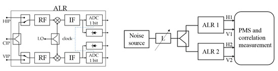
Figure 5.
Left: Simplified block diagram of an Advanced Receiver for the Future L-Band Radiometer (ALR). Labels HIP, VIP, and CIP refer respectively to the Horizontal, Vertical, and Calibration Input Planes. The additional position of the input switch to a matched load and IF switched attenuation, needed for offset measurement, are not shown for simplicity. Right: Test bench to measure the cross-correlation and power of a baseline formed by two ALR units.
The test bench uses two different ALR units driven by correlated noise provided by a single source and a power divider (see Figure 5, right). Eleven levels are injected in-phase to both units by means of a variable attenuator. Within each ALR unit, the input power is further divided into both H and V channels, as seen in the block diagram at the left of the figure. The digitized output signals are sent to a data processing unit (labeled “PMS and correlation measurement” in the figure) that includes one-clock delays to get the Q signals. The data processing unit includes a matrix of 1-bit two-level digital correlators [13] to compute all correlation pairs between the different ALR output digital signals (H1, V1, H2, V2), including self-IQ for each one. Correlation with additional delays to measure the fringe washing function shape are also implemented. The analog detected output from the diode is converted to a square signal by a voltage to a frequency converter. Both correlation and power data are saved in text files for further processing by a dedicated software.
3.1. Power Measurements
Figure 6 shows the noise equivalent temperature injected at each ALR unit for all eleven levels. The twelfth one corresponds to switching all inputs to matched resistors (not shown in Figure 5) in order to inject ambient uncorrelated noise. The level of noise at each level is computed from the S-parameters of the noise distribution network, measured independently, and the Excess Noise Ratio (ENR) of the source using the procedures of [14]. The insertion loss of the switches inside the ALR units was also taken into account in order to provide the level of noise at the Horizontal Input Plane (HIP) and VIP, respectively (see Figure 5, left). As seen in Figure 6, the noise distribution network is highly symmetrical and injects the same amount of noise to both units.
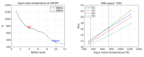
Figure 6.
Left: Noise equivalent temperature injected at the HIP/VIP for each level. Right: Corresponding PMS measurements by all receivers.
In the same figure, right, the PMS output is shown as a function of the injected power. Units are kHz due to the voltage-to-frequency converter implemented in the PMS. As seen, all four chains show high linearity and similar gains. Using the four-point technique [15] with the hot and warm points marked in the figure, the parameters summarized in Table 1 are obtained. All four receiver chains have similar parameters with a somewhat better noise figure in the case of ALR Unit 1. Both the gain and noise figure are referenced to the HIP/VIP (see Figure 5).

Table 1.
Parameters of PMS characterization.
3.2. Correlation Measurements
The correlation counts measured by the setup of Figure 5 are first converted to the normalized correlation of the input Gaussian signals using the same method as for the MIRAS instrument on board SMOS and detailed in Equation (2) of [9]. This first step needs the measurement of the correlation of all signals with all ones and all zeroes in order to calibrate the correlator offset. While in MIRAS, this correction was important (see Figure 14 of [10]), in this case, this correction was shown to be almost negligible due to the improved design of the samplers and the correlators. Figure 7 shows the percentage of zeroes and ones in all signals and also the estimated offset due to the zero-one unbalance expressed in correlation units (cu), defined as . Results for all I and Q signals are provided; however, as expected, the zero-one unbalance for any Q signal is identical to the corresponding I signal since they are both the same, and only a delay is introduced to get one from the other.
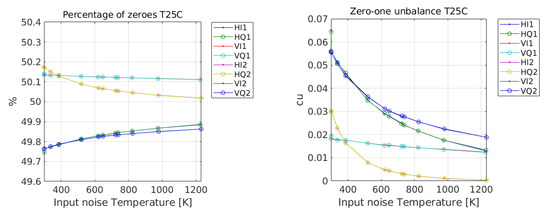
Figure 7.
Percentage of zeroes and estimated samplers offset as a function of the total noise temperature at the HIP/VIP.
3.2.1. Self-IQ Correlation
Figure 8 shows the correlations measured between the I and Q signals of each receiver with this last one obtained just by delaying one clock. According to the theoretical predictions of Section 2.4.2, this correlation is related to the center frequency of the signal. The plot on the left shows the measured correlation and the plot on the right the estimated center frequency according to (26), both as a function of the total input power at each level provided in Figure 6. The nominal value (11) MHz is marked with a dashed line. These results confirm that the center frequency error can be measured by this technique and show that it is small in all units, ranging in this case from about 900 kHz to −60 kHz. It is observed that Unit 2 is better centered in the nominal intermediate frequency in both channels.
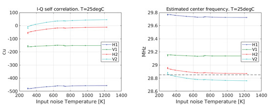
Figure 8.
Self-IQ correlation and estimated center frequency. The average errors with respect to the nominal value are 890.6, 294.0, 43.4, and −58.6 kHz for receivers H1, V1, H2, and V2, respectively.
3.2.2. Cross-Correlation
The complex cross-correlation, both nominal and redundant, is computed out of the raw measurements provided by the setup of Figure 5 according to Equations (20) and (21) and using the approximation (28), the nominal bandwidth, and the center frequency error estimated in Figure 8. Figure 9 shows the results in amplitude (correlation units) after averaging nominal and redundant retrievals as a function of the correlated input noise temperature (48). Shown also in the plot (circles) is the expected theoretical cross-correlation computed using Equation (29) of [14], repeated here for convenience:
where is the “correlated input temperature”, also used in the horizontal axis of the figure and defined as:
where is the noise temperature of the source determined from its excess noise ratio, the physical temperature of the network, assumed constant and measured simultaneously with a sensor, and the S-parameters of the noise injection network when the noise source is in port 0. They were independently measured by a network analyzer. The system temperatures in (47) are computed as:
where the receiver noise temperature is the one in Table 1 retrieved with the four-point technique. Finally, the term in (47) is the fringe washing function at the origin, computed from the four-point characterization directly with Equation (15) of [16]. Retrieved values for all six baselines are given in Table 2.
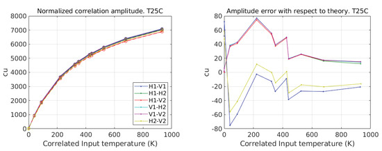
Figure 9.
Left: Amplitude of the normalized correlation after correction and theoretical values in circles. The right plot shows the error with respect to the theoretical values. The legend of the left plot applies.
Table 2.
Measured fringe washing function at the origin.
As seen in Figure 9, the consistency between measured and corrected correlations and theory is remarkable, even though the S-parameters used in the computations are only approximate. Referring to Figure 5, the actual measurements using a network analyzer were only done for the external part of the distribution network. All the part that is inside the ALR to be divided into both H and V chains is only approximated by a fixed 5-dB loss, and no phase is available. Furthermore, the isolation parameters between these inner ports was not measured.
Figure 10 shows the phase of the complex correlation as a function of correlated input temperature. As seen, it is almost constant for all baselines with variations lower than , except for the baseline H1-V1, which has a larger variation. For low values of input power, the uncertainty in the phase is very large, as expected.
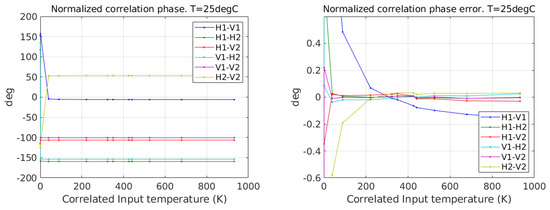
Figure 10.
Phase of normalized correlation. The right plot shows the same phase with the average removed to see the variations.
3.2.3. Fringe Washing Function Shape
Equations for retrieving the fringe washing function are derived in Section 2.5. They are based on introducing additional delays to each one of the signals and measuring the corresponding correlation. This feature has been implemented in the setup of Figure 5, and the results are given below. Figure 11 shows the measured real correlation between signals H1 and V1 for Noise Level 6 (see Figure 6) at the seven time delays specified in Equations (36)–(42). For points where there are two measurements (all except the first and the last ones), the average value is used. The theoretical value computed from (45) is drawn in the same figure using first-guess values of the unknown parameters. Specifically, and are the amplitude and phase of the correlation obtained in Section 3.2.2; and B are set to their nominal values; and is set to zero. As seen, even though using approximate parameters, the measured values of correlation match quite well with the theoretical expectations.
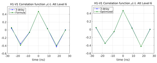
Figure 11.
Correlation function measured at different delays. On the left, it is compared with the theoretical formula using initial parameter values. On the right, after optimizing the parameters.
In the plot on the right, the result of a numerical optimization of these parameters is shown. In this case, both lines just superimpose each other, indicating that the correct parameters have been found. Parameters for the fringe washing function shape are then computed as indicated after Equation (46).
The procedure was repeated for all baselines, resulting in the parameters specified in Table 3.
Table 3.
Measured fringe washing function shape parameters. cu, correlation units.
As expected, the A parameter is close to unity for all baselines. The B parameter is the actual signal bandwidth retrieved by this procedure and is compatible with a nominal value of 19 MHz. The parameter C represents the differential group delay between the two receivers forming the baseline. It is of the order of some nanoseconds in all cases and some of them out of the one-sigma margin obtained in SMOS-LICEF, probably due to the lack of symmetry of the H and V channels. Finally, the E parameter is the center frequency displacement and is compatible with the values obtained for each receiver individually in Section 3.2.1.
As an example of the shape of the fringe washing function, Figure 12 shows the plot for two baselines (H1-H2 and V1-V2). The vertical lines indicate plus/minus the clock period. As seen, the decorrelation for this delay is not negligible, and the effect of group delay is noticeable in the shift of the maximum of the function.
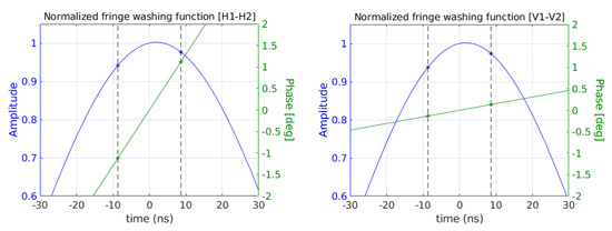
Figure 12.
Normalized fringe washing function for baselines H1-H2 and V1-V2. The rest of the baselines have similar functions.
3.2.4. Sensitivity Circles
In order to assess the correct retrieval of the correlation phase, a test was performed by changing the phase of the local oscillator by steps of 30 deg from zero to 360. This change must be reflected in the phase of the measured correlation, so that the result must be a circle centered at the origin. Failure to calibrate correctly will result in a distorted circle, as for example an ellipse. This test is important to check that the decorrelation of the imaginary part mentioned in Section 2.4.1 is well corrected by the procedure proposed.
Figure 13 shows the results for a circle corresponding to injecting about 15k of correlated noise. Only four baselines are shown since the local oscillator distribution between the H and V channels within the ALR is fixed, and its phase cannot be changed. These are applied only to baselines formed by ALR 1 and ALR 2. As seen, for all baselines, a circle is correctly retrieved. The radius and the center is indicated in the figure.
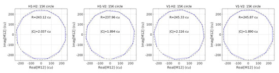
Figure 13.
Sensitivity circles.
3.3. Effective Integration Time
For the proposed digital IQ demodulation, the sampling rate must be set equal to four times the center IF. This is larger than the minimum Nyquist rate of twice the signal bandwidth, so some level of oversampling is present, which is beneficial in terms of noise reduction. The effective integration time taking into account actual filters’ response and one-bit digital correlator is estimated as a function of the sampling frequency using the method outlined in [17]. The result for the parameters of the hardware designed are provided in Figure 14, left. It should be pointed out that the filters used in this simulation are prototypes measured for SMOS, not the actual units used in the ALR, so some discrepancy is expected. As seen, the oversampling allows having an effective integration time of about times the actual value for the sampling frequency of used in the test. This result is much better than the ratio of of SMOS [17]. Note the local maximum at MHz and also the stabilization after about 80 MHz, compatible with twice the maximum frequency of the signal spectrum MHz. For an ideal case of no quantization and ideal rectangular filters, the effective integration time is equal to the actual one in these two cases and keeps constant beyond the last one.
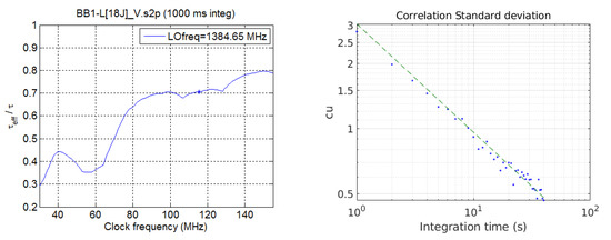
Figure 14.
Left: Effective integration time as a function of clock frequency. The actual clock is marked with a star. Right: Standard deviation of measurements as a function of integration time.
The right plot of Figure 14 shows the measured variance of the correlation for uncorrelated input signals corresponding to baseline H1 V1as a function of integration time. These data were obtained by continuously measuring the PMS and correlation during a couple of hours using the setup of Figure 5. Drawn in the same plot also is a straight line corresponding to the expected standard deviation using the theoretical effective integration time of . The agreement is quite considerable, and even the measured standard deviation for a 1-s integration time is smaller than expected theoretically. According to these measurements and using the result for a 1-s integration time, the effective integration time is about times the actual one.
4. Discussion
The ALRs are the new receiving units currently being developed for a follow-on SMOS operational mission. They include a number of improvements with respect to the LICEF presently implemented in SMOS. One of the main differences between both is that the analog phase/quadrature mixer of the LICEF is substituted in the ALR by a digital design based on a simple one-clock delay. This difference has to be taken into account for the correct formulation of the complex correlation and to properly define its requirements. Most of the equations used in the SMOS level 1A data processing [9] are no longer valid, and they have to be substituted by the ones developed here in Section 2. The new formulation is based on the equations governing the cross-correlation of Gaussian random signals and is rigorous. It provides the expected values of the correlation for given input signals and proposes an analytical method to correct for the two errors associated with this technique: center frequency and decorrelation.
The technique makes no assumption regarding the type of digital correlator used, but in this paper, it is specifically applied to a one-bit two-level design. It is the one implemented in SMOS and has the advantage of simplicity and easiness to fabricate large correlator arrays needed for an instrument with a large number of elements such as SMOS or its future version.
Experiments using correlated noise injection are very encouraging as they demonstrate that the digital technique is able to measure both amplitude and phase just as the analog counterpart. Furthermore, the proposed error correction technique compensates effectively the distortion of raw measurements, as clearly demonstrated by the recovery of perfect circles in the complex plane when only the phase of the local oscillator is changed (Figure 13). Moreover, the cross-correlation amplitude as a function of the input power is found to behave in a compatible manner with the expected one computed from only the noise distribution network characterization. The small discrepancies found can be attributed to uncertainties in the distribution network. The fringe washing function at the origin, which is actually the correlator complex gain, is successfully retrieved.
The equations presented predict that the autocorrelation of a given signal is directly related to the center frequency difference with respect to the nominal one. This is perfectly demonstrated experimentally by retrieving the actual center frequency in all four channels characterized (Figure 8).
The fringe washing function accounts for signal decorrelation due to a finite bandwidth. In any interferometric radiometer, especially if it includes large baselines, it has to be taken into account in the image reconstruction process. Moreover, in the proposed digital IQ demodulator, this function has also an impact on the decorrelation of the imaginary part. A simplified guess of this function is obtained just from the signal bandwidth, but for better results, it must be measured using delays introduced in the signals. The technique is already applied to SMOS where delays at plus and minus the sampling period are periodically introduced in all calibration events performed every two months [18]. The same strategy cannot be implemented when the digital IQ demodulator is used since the Q signal is already delayed. However, a method based on extra delays is proposed in this paper and allows measuring the fringe washing function shape after a fast optimization procedure. Experimental results are provided in Section 3.2.3 demonstrating that the measured correlation function is well described by the theoretical development. Furthermore, as a result of the optimization, an improved value of the cross-correlation is obtained, both in amplitude and in phase, which could be the basis for defining still an enhanced method to get the complex correlation in future developments. In any case, the fringe washing function shape to be applied in the image reconstruction processor is clearly retrieved with the method proposed.
The sampling rate at four times the center IF frequency assures a large effective integration time, estimated to about 0.8 times the actual one when using a 1-bit two-level correlator, much larger than the case of SMOS, so reducing the thermal noise associated with the correlation measurement and ultimately improving the radiometric sensitivity.
5. Conclusions
Digital IQ demodulation is successfully implemented in a baseline of an interferometric radiometer by a one-clock delay of the output IF signal of one receiver with respect to the other. If the sampling frequency is chosen as four times the center IF frequency, for a narrow-band signal, this schema provides approximately the correct complex cross-correlation. The quadrature error of analog IQ demodulators is no longer present, but two new ones appear: the center frequency error and the decorrelation of the imaginary part. Both of them are successfully corrected by data processing based on the new formulation presented. In a simplified version, only the nominal signal bandwidth is needed as additional information, but the complete one needs to know the normalized fringe washing function. A technique to retrieve this function using additional delays is proven to be robust and to provide accurate values for this function, which can be ultimately used to improve the correlation measurements. The experimental results in a single baseline are highly consistent with the theoretical predictions and provide a solid path in the development of a large instrument, eventually to take over the successful SMOS mission for Earth observation.
Author Contributions
Conceptualization, I.C. and M.M.N.; methodology, M.M.N., I.C., and R.V.; software, I.C. and R.V.; validation, M.M.N. and A.C.; formal analysis, I.C. and M.M.N.; investigation, I.C., M.M.N. and R.V.; resources, R.V. and A.C.; data curation, R.V. and A.C.; writing—original draft preparation, I.C.; writing—review and editing, M.M.N., R.V., and F.T.; visualization, I.C.; supervision, F.T.; project administration, A.C., M.S., and I.C.; funding acquisition, M.S., M.M.N., and F.T. All authors read and agreed to the published version of the manuscript.
Funding
This research was funded by the European Space Agency through Subcontract ALR-RP-0017-TA with SENER TAFS S.A.U. (Barcelona-Spain) and by Ministerio de Economía, Industria y Competitividad, Gobierno de España, Project TEC2017-88850-R.
Institutional Review Board Statement
Not applicable.
Informed Consent Statement
Not applicable.
Data Availability Statement
Not applicable.
Conflicts of Interest
The authors declare no conflict of interest.
Abbreviations
The following abbreviations are used in this manuscript:
| ALR | Advanced Receiver for the Future L-Band Radiometer |
| DUT | Device Under Test |
| ESA | European Space Agency |
| EBB | Elegant Breadboard |
| IF | Intermediate Frequency |
| IQ | In-phase and Quadrature |
| LICEF | Lightweight Cost-Effective Front-end |
| LO | Local Oscillator |
| MIRAS | Microwave Imaging Radiometer with Aperture Synthesis |
| NOSU | Noise Source |
| PMS | Power Measurement System |
| RF | Radio Frequency |
| SMOS | Soil Moisture and Ocean Salinity |
Appendix A. The Fringe Washing Function
Given two receivers k and j, the fringe washing function with respect to an arbitrary reference frequency is defined as (see [6]):
where are the receivers’ frequency responses normalized to their maximum value and their noise-equivalent bandwidths defined as:
Equation (A1) is the inverse Fourier transform of the conjugated product of the receivers’ frequency responses (for positive frequencies) shifted to the origin by an amount equal to . For a single receiver, a fringe washing function can also be defined by collapsing in (A1) both frequency responses into one:
The fringe washing function is in general complex and has the following general properties:
- If the product is real, then , so the real part is even and the imaginary part odd. This happens either if both receivers have identical frequency responses or if a single receiver is considered (the case of or ).
- If both frequency responses are symmetrical around the reference frequency (that is, if ), then the fringe washing function is real.
- A group delay difference between both receivers, defined as , is equivalent to a linear phase shift in the frequency domain. As a consequence, the integrand of (A1) can be written as the product of two filter responses with equal group delay multiplied by . After some mathematical operations, it is easily found that the fringe washing function becomes:where is the fringe washing function corresponding to filters with equal group delay. As expected, this result is compatible with adding a delay of to (8).
- Changing the reference frequency of the fringe washing function only adds a linear term to the phase, with no change in the amplitude:
- If the product can be approximated by a rectangular function of width B centered at , then the fringe washing function referenced to this frequency becomes:simplifying to just if . For filters centered at another frequency, (A5) applies.
- Independent of the reference frequency, the fringe washing function at the origin is:which is complex in general and normally has an amplitude close to unity (if the filters are similar enough).
References
- Barré, H.; Duesmann, B.; Kerr, Y. SMOS: The mission and the system. IEEE Trans. Geosci. Remote Sens. 2008, 46, 587–593. [Google Scholar] [CrossRef]
- McMullan, K.; Brown, M.; Martín-Neira, M.; Rits, W.; Ekholm, S.; Marti, J.; Lemanzyk, J. SMOS: The payload. IEEE Trans. Geosci. Remote Sens. 2008, 46, 594–605. [Google Scholar] [CrossRef]
- Martín-Neira, M.; Oliva, R.; Corbella, I.; Torres, F.; Duffo, N.; Durán, I.; Kainulainen, J.; Closa, J.; Zurita, A.; Cabot, F.; et al. SMOS instrument performance and calibration after six years in orbit. Remote Sens. Environ. 2016, 180, 19–39. [Google Scholar] [CrossRef]
- Martín-Neira, M.; Goutoule, J.M. MIRAS A Two-Dimensional Aperture-Synthesis Radiometer for Soil Moisture and Ocean Salinity Observations. ESA Bull. 1997, 95–104. [Google Scholar]
- Zurita, A.M.; Corbella, I.; Martín-Neira, M.; Plaza, M.A.; Torres, F.; Benito, F.J. Towards a SMOS Operational Mission: SMOSOps-Hexagonal. IEEE J. Sel. Top. Appl. Earth Obs. Remote Sens. 2013, 6, 1769–1780. [Google Scholar] [CrossRef]
- Corbella, I.; Duffo, N.; Vall-llossera, M.; Camps, A.; Torres, F. The visibility function in interferometric aperture synthesis radiometry. IEEE Trans. Geosci. Remote Sens. 2004, 42, 1677–1682. [Google Scholar] [CrossRef]
- Dugundji, J. Envelopes and Pre-Envelopes of Real Waveforms. IRE Trans. Inf. Theory 1958, 4, 53–57. [Google Scholar] [CrossRef]
- Franks, L.E. Signal Theory; Prentice Hall, Inc.: Upper Saddle River, NJ, USA, 1969. [Google Scholar]
- Corbella, I.; Torres, F.; Camps, A.; Colliander, A.; Martín-Neira, M.; Ribó, S.; Rautiainen, K.; Duffo, N.; Vall-llossera, M. MIRAS End-to-End Calibration. Application to SMOS L1 Processor. IEEE Trans. Geosci. Remote Sens. 2005, 43, 1126–1134. [Google Scholar] [CrossRef]
- Corbella, I.; Torres, F.; Duffo, N.; Martín-Neira, M.; González-Gambau, V.; Camps, A.; Vall-llossera, M. On-Ground Characterization of the SMOS Payload. IEEE Trans. Geosci. Remote Sens. 2009, 47, 3123–3133. [Google Scholar] [CrossRef]
- Corbella, I.; Torres, F.; Duffo, N.; Duran, I.; González-Gambau, V.; Martín-Neira, M. Wide Field of View Microwave Interferometric Radiometer Imaging. Remote Sens. 2019, 11, 682. [Google Scholar] [CrossRef]
- Camps, A.; Torres, F.; Corbella, I.; Bará, J.; Monzón, F. Automatic calibration of channels frequency response in interferometric radiometers. Electron. Lett. 1999, 35, 115–116. [Google Scholar] [CrossRef]
- Hagen, J.B.; Farley, D.T. Digital-correlation techniques in radio science. Radio Sci. 1973, 8, 775–784. [Google Scholar] [CrossRef]
- Corbella, I.; Camps, A.; Torres, F.; Bará, J. Analysis of noise injection networks for interferometric radiometer calibration. IEEE Trans. Microw. Theory Tech. 2000, 48, 545–552. [Google Scholar] [CrossRef]
- Piironen, P. PMS Offset Determination Using an IF Attenuator; Technical Note 14629/00/NL/SF; ESA-ESTEC: Noordwijk, The Netherlands, 2002. [Google Scholar]
- Torres, F.; Corbella, I.; Camps, A.; Duffo, N.; Vall-llossera, M.; Beraza, S.; Martín-Neira, M. Denormalization of Visibilities for In-orbit Calibration of Interferometric Radiometers. In Proceedings of the International Geoscience and Remote Sensing Symposium, IGARSS 2005, Seoul, Korea, 25–29 July 2005; Volume VIII, pp. 5554–5557. [Google Scholar]
- Corbella, I.; Torres, F.; Camps, A.; Bará, J.; Duffo, N.; Vall-llossera, M. L-band aperture synthesis radiometry: Hardware requirements and system performance. In Proceedings of the International Geoscience and Remote Sensing Symposium, IGARSS 2000, Honolulu, HI, USA, 24–28 July 2000; Volume 7, pp. 2975–2977. [Google Scholar]
- Brown, M.; Torres, F.; Corbella, I.; Colliander, A. SMOS calibration. IEEE Trans. Geosci. Remote Sens. 2008, 46, 646–658. [Google Scholar] [CrossRef]


Publisher’s Note: MDPI stays neutral with regard to jurisdictional claims in published maps and institutional affiliations. |
© 2021 by the authors. Licensee MDPI, Basel, Switzerland. This article is an open access article distributed under the terms and conditions of the Creative Commons Attribution (CC BY) license (http://creativecommons.org/licenses/by/4.0/).