Article

A Bayesian Model to Forecast the Time Series Kinetic Energy Data for a Power System

by
Ashish Shrestha
1,*,
Bishal Ghimire
2 and
Francisco Gonzalez-Longatt
1
1
Department of Electrical Engineering, Information Technology and Cybernetics, University of South-Eastern Norway, 3918 Porsgrunn, Norway
2
Department of Electrical and Electronics Engineering, Kathmandu University, Dhulikhel 45200, Nepal
*
Author to whom correspondence should be addressed.
Energies 2021, 14(11), 3299; https://doi.org/10.3390/en14113299
Submission received: 3 May 2021 / Revised: 26 May 2021 / Accepted: 2 June 2021 / Published: 4 June 2021

Abstract

:
Withthe massive penetration of electronic power converter (EPC)-based technologies, numerous issues are being noticed in the modern power system that may directly affect system dynamics and operational security. The estimation of system performance parameters is especially important for transmission system operators (TSOs) in order to operate a power system securely. This paper presents a Bayesian model to forecast short-term kinetic energy time series data for a power system, which can thus help TSOs to operate a respective power system securely. A Markov chain Monte Carlo (MCMC) method used as a No-U-Turn sampler and Stan’s limited-memory Broyden–Fletcher–Goldfarb–Shanno (LM-BFGS) algorithm is used as the optimization method here. The concept of decomposable time series modeling is adopted to analyze the seasonal characteristics of datasets, and numerous performance measurement matrices are used for model validation. Besides, an autoregressive integrated moving average (ARIMA) model is used to compare the results of the presented model. At last, the optimal size of the training dataset is identified, which is required to forecast the 30-min values of the kinetic energy with a low error. In this study, one-year univariate data (1-min resolution) for the integrated Nordic power system (INPS) are used to forecast the kinetic energy for sequences of 30 min (i.e., short-term sequences). Performance evaluation metrics such as the root-mean-square error (RMSE), mean absolute error (MAE), mean absolute percentage error (MAPE), and mean absolute scaled error (MASE) of the proposed model are calculated here to be 4.67, 3.865, 0.048, and 8.15, respectively. In addition, the performance matrices can be improved by up to 3.28, 2.67, 0.034, and 5.62, respectively, by increasing MCMC sampling. Similarly, 180.5 h of historic data is sufficient to forecast short-term results for the case study here with an accuracy of 1.54504 for the RMSE.

1. Introduction

With the increasing concern over clean and sustainable energy and rapid growth in electronic power converter (EPC)-based technologies, modern power systems are experiencing vast transformation in all sectors, including generation, transmission, distribution, and even utilization. The generation sector is presently integrating EPC-based renewable energy resources (RESs), including photovoltaic panels and wind turbines, whereas the control mechanisms of other sectors are dependent on EPCs. At the same time, the proportion of synchronous generators is reducing in modern power systems, and synchronous generators are considered to be the main source of system inertia. In comparison to the conventional operation mode, the huge penetration of EPC-based technologies presents several changes in the operating dynamics of a modern power system. The major change is a significant drop in system inertia, which may directly affect the frequency quality, and operational security of power supply [1,2]. Frequency quality has an important role regarding the smooth operation of a power system, where low system inertia can initiate accidental system blackouts [3]. Furthermore, the transient stability of a modern power system is also highly sensitive to the penetration level of EPC-based technologies, along with the given fault location and its severity [4].
Estimating power system performance indicators is an important task that must be conducted for the secure and reliable operation of a power system, especially after disturbance. Numerous studies have been conducted and many are still in the research and development phase to obtain the best solution for estimating system inertia and securing a power system from potential disturbances. Most of studies have focused on frequency quality measurement and monitoring techniques which are further used to estimate the inertia. The work in [5] presented an ambient wide-area measurement technique to estimate power system inertia, in which the authors took the ambient frequency and the active power of the power system by using phasor measurement units (PMU). Similarly, Zhang et al. proposed a synchrophasor measurement-based method to estimate the equivalent inertia of a system containing a wind power plant [6]. Fereidouni et al. proposed an online security assessment tool for the South West Interconnected System in Australia, which monitored and forecasted system inertia on an online basis and estimated parameters such as load damping factors and demand-side inertia [7]. Dynamic regressor extension and mixing procedures have been proposed with the aim to develop an online estimator of power system inertia. In such case, some authors have used a non-linear and aggregated power system model [8]. A swing equation and PMU-based inertia estimation technique for wind power plants has been proposed, where the synchrophasor measurements are taken from a real-time digital simulator using industrial PMUs [9]. Similarly, another study has utilized frequency and voltage response just after disturbance to estimate the inertia by combining two separate approaches (i.e., R for the frequency response and V for the power change due to the load voltage dependency) [10].
The main complication for system inertia estimation methods is that the inertial response between controllers and stabilizers cannot be distinguished, and the system dynamics cannot be analyzed during the normal operation [5]; however, there have been no attempts to estimate system inertia more accurately by forecasting the continuously available data from the power system, such as kinetic energy and power deviations. As such, the discussed issues can be addressed in a more practical way. There are some research articles in which system frequency, nadir frequency, power generation, and load have been used to forecast system performance [11,12,13]. A number of studies have been conducted to forecast the short-term time series data of load as an indicator for a power system [14,15,16]. A previous paper from the authors presented a structural time series-based model to forecast the kinetic energy of a power system for a short period, which concluded that the identified value of kinetic energy can be used to estimate the system inertia on a real-time basis [17]. This research article is based on further investigation of that research article and presents a new forecasting method to estimate system performance indicators. Though described in detail further below, the following summarizes the main contributions of this paper:
(a)
A Bayesian model used to forecast the univariate time series data of kinetic energy is presented. One year of data for the kinetic energy of the INPS are used to forecast for the next 30 min of data. The results of the presented model are evaluated with other performance metrics and are found to within acceptable limits. Further, the results are cross-checked with the results of the ARIMA model.
(b)
The optimum training dataset size required to forecast 30-min values of the kinetic energy via an optimization technique is identified. There may be a considerable number of historical data, and this will result in a greater computational time if all of the data are used in the forecasting process. It is also very important to obtain results as quickly as possible, since decisions (i.e., control actions) must be made at the right time. Hence, determining the optimal training dataset size could be significant in terms of optimizing the required computational time and memory.
The authors of this paper aim to present a method that forecasts the time series data of kinetic energy as an important parameter of a power system. A dataset containing a year of time series data for the INPS (1 sample per minute) is used to forecast short-term results (i.e., the next 30 min) using the Bayesian model presented here. The forecasted time series data of the kinetic energy can be utilized to estimate the system indicators and manage the whole system during normal operation, as well as in case of contingencies. This paper first introduces the background and the problems that arise because of the huge penetration of EPC-based technologies in power grids. The issues regarding a modern power system with massively EPC-based technologies are briefly discussed. In Section 2, the adopted methodologies are described in detail. The models for time series forecasting, their mathematical formulations, and the performance measurement metrics are additionally discussed in detail. Section 3 presents the results of this paper. Finally, the conclusions of this work are presented in Section 4.

2. Methodology

This section is focused on the description of the adopted methodology, which can be seen in Figure 1. A detailed description of the adopted methodology may be seen below.

2.1. Data Types and Preparation

The data for the kinetic energy of the INPS for 2019 were taken from the web portal of FINGRID (Finland’s transmission system operator). Data were collected each minute, amounting to 525,604 samples in total. The minimum and maximum values of the kinetic energy in 2019 were recorded as 126 GW and 273 GW. Similarly, the mean and median values of the total samples were obtained to be 194.1 GW and 191 GW with a standard deviation of 27.6.
It is important to have reliable and accurate data to correctly analyze performance and visualize results. Incorrect visualization is a result of unreliable data and may mislead viewers. Hence, the raw data here were first processed to minimize possible errors by filtering and fulfilling missing values. In this study, the raw sample sets were passed through a kernel filter to reject errors and a regression impulsion method was used to fulfil the missing values. Overall, 9273 samples were missed among the total set of 525,604 samples (i.e., 1.76%), which were then fulfilled via the regression impulsion method.

2.2. Model Selection

The samples that the authors took were of a univariate type, and the best way to analyze univariate data is with a structural time series model. Various research articles [18,19] have presented structure time series models based on the concept of decomposition for univariate samples. Authors have segregated time series data into different components, like the trend, seasonal, and irregular components. In this research article, the authors adopted the same concept of the structural time series model and decomposed the whole time series model into three components as shown in Equation (1).
y ( t )   =   g ( t )   +   s ( t )   +   ϵ t
where g(t) is the logistic growth (i.e., trend of the data), s(t) is periodic changes, and ϵt is the error that provides some random nature of the result. In the presented model, the logistic growth is just a regressor of time with several linear and non-linear fitting and calculated by using Equation (2). In Equation (2), C is the carrying capacity, r is the growth rate, and m is the offset parameter.
g ( t )   =   C 1 + e r ( t m )
The carrying capacity and growth rate are not constant values and instead vary with time. Incorrect assumptions may lead to incorrect interpretations. Hence, time-dependent carry capacity (i.e., Ct) and growth rate (i.e., rt) were considered. Now, the revised relation for the logistic growth is given by Equation (3).
g ( t )   =   C t 1 + e ( r + a [ t ] T δ ) ( t m a [ t ] T   Υ )
where δ is the rate of change within the rate adjustment vector (δ ϵ ℝS) with Sj change points and Υ is the adjustment correction vector for offset parameters. Similarly, a[t]T is a vector which is defined as below:
a j [ t ]   =   {   1 ,   i f   t   S j ,   0 ,   | O t h e r w i s e   a n d   a j [ t ]   ϵ   ( 0 , 1 ) S
Similarly, the seasonal variation s(t) of the time series parameters can be determined using the Fourier series given in Equation (5). The seasonal variation contains multi-period constraints, such as seasonal changes and human behaviors, which cannot be forecasted by the logistic growth accurately, hence the Fourier series is used to model the periodic functions of time. In the presented model, the parameters (i.e., a1, b1, a2, b2, …, aN, bN) with the N Fourier order are used in modeling to identify the seasonal variation for P period.
s ( t )   =   n = 1 N ( a n c o s 2 n π t P + b n s i n 2 n π t P )
After segregating the time series data into three components, the authors implemented a Bayesian model to forecasting the time series data of kinetic energy. A Bayesian model was selected for this study because it forecasts the future by using a combination of available information and a source of uncertainty in the form of a predictive distribution with improved accuracy. Later, the ARIMA model was used to compare the results of these two models. The details of these two models are discussed below.

2.2.1. Bayesian Approach

Bayes theorem is widely used in the field of data analysis and is often used to analyze the conditional probability of numerous events, such as forecasting hierarchically structured time series data [20], seasonal time series data [21,22], multi-step-ahead time series prediction [23], general estimation and prediction [24], and statistical analysis [25,26]. A Bayesian approach has been presented to forecast univariate time series data by implementing a technique of sampling the future in [27]. A Bayesian time series forecasting model with the change point and anomaly detection was proposed in [28], where the authors implemented an iterative algorithm with a Kalman filter and smoothing in their analysis, along with a Markov chain Monte Carlo (MCMC) method. Maarten et al. presented that learning Bayesian networks could be used to analyze the time series data of clinical parameters and concluded that the model learning methods could find a good predictive model with a reduced computational time and good interpretation [29]. In [23], the combination of a Kalman filtering model and echoing neural networks was used to predict multi-step-ahead time series data (i.e., a dynamic Bayesian network). Panagiotelis et al. presented a Bayesian density method to forecast intraday electricity prices by using multi-variate skewed t-distributions and a MCMC method [30]. Not only these but there are also the diverse applications of the Bayes theorem.
Theoretically, in Bayes theorem, if X and Y are two events, then the probability of event X with the occurrence of event Y can be calculated using Equation (6). This is the joint probability of two events and does not suggest symmetrical characteristics. In Equation (6), Bayes theorem is defined with the following terms: P(X|Y), posterior probability; P(X), prior; P(Y|X), likelihood; and P(Y), evidence. If the value of the prior, likelihood, and evidence is known, the posterior probability can be calculated mathematically.
P ( X | Y )   =   P ( X ) ·   P ( Y | X ) P ( Y ) ,   for   P ( Y )   0
For the specific case of kinetic energy, the relation for the joint distribution over the random inputs is described by Equation (7). Here, P indicates the joint probability distribution function for the conditional probability in the form of P(KE|pa(KE)), where KEi (KEi ϵ KE) denotes the variables to be analyzed (i.e., kinetic energy) with the influence of their parent variables pa(KEi). The parent variables include the historical values of the parameter (i.e., historical values of KE), which must be considered during the forecasting of new values.
P ( K E 1 ,   K E 2 ,   K E 3 ,   ,   K E n )   =   i = 1 n P ( K E i   | p a ( K E i ) )
In the conventional manner of estimation via linear regression, Equation (8) is applied with the normally distributed error (ϵt~Normal(0, σ2)); however, by using Bayes theorem, the estimation can be made more accurate, since, in estimation, Bayesian theory minimizes the posterior expected values of the loss function. In a single sentence, the Bayesian model minimizes the posterior expected loss and maximizes the posterior expectation of a given function. By adopting the Bayes theorem in the linear regression, Equation (9) presents the revised posterior distribution, and Equation (10) gives the likelihood function. In the equations, β is the coefficient and σ2 is the variance.
Y t   =   B X t   +   ϵ t
H(β, σ2|Yt) ∞ F(Yt|β, σ2) * P(β, σ2)
F ( Y t | β , σ 2 ) = ( 2 π σ 2 ) T / 2   e   ( Y t β X t ) T   ( Y t β X t ) 2 σ 2
As given by Equation (6), the probabilities of conditional events can be identified if the values of the other three parameters are known. In this paper, the authors have calculated the probability of a posterior event and applied it in the forecasting of kinetic energy by using Stan’s limited-memory Broyden–Fletcher–Goldfarb–Shanno (LM-BFGS) [31] algorithm as an optimization technique. The LM-BFGS algorithm is very popular in parameter estimation applications and is a quasi-network method, which approximates the BFGS algorithm by utilizing the potential less memory and computational time. The main objective of LF-BFGS is to minimize the unhindered errors within functions. Also, the new value ( x t + 1 ) can be obtained using Stan’s LM-BFGS algorithm as given in Equation (11) [32], where α t is the step length that should be satisfy the Wolfe conditions (i.e., sufficient decrease and curvature conditions in line searching method), ∇ f t is the gradient, and H t is the updated Hessian approximation (n*n symmetric) at the iteration.
x t + 1 = x t α t H t f t
In the LM-BFGS algorithm, the estimation of H t is quite sensitive, which determines the accuracy and efficiency of the model. In comparison to a BFGS algorithm, the LM-BFGS algorithm is capable of computing problems in large iterations with less cost and storage by maintaining simple and compact approximations [32]. The workflow that was followed for the LM-BFGS algorithm in this study is shown in Figure 2. In this approximation, the vector pair in the set of ( s i , y i ) is replaced by the newest set of pairs ( s t , y t ) at each new iteration and is updated accordingly. For example, if the latest iteration is x t , then the set of vector pair will be ( s i , y i ) at the t-th iteration (i = tm, …, t − 1). The initial Hessian approximation H t 0 is considered and continuously identifies updates up to t-th iteration until H t satisfies the relationship given in Equation (12).
H t = ( V t 1 T     V t m T )   H t 0   ( V t m V t 1 ) + ρ t m   ( V t 1 T   V t m + 1 T )   s t m s t m T ( V t m + 1 V t 1 ) + ρ t m + 1   ( V t 1 T   V t m + 2 T )   s t m + 1 s t m + 1 T ( V t m + 2 V t 1 ) + + ρ t 1   s t 1 s t 1 T
where, ρ t   = 1 y t T   s t   , V t   = I ρ t s t T y t , s t = x t + 1 x t , and y t = f t + 1   f t .
Further, a MCMC method is used as a No-U-Turn sampler in this study. With an auxiliary variable u and target distribution f( θ ), Equation (13) is used to find the sample θ , and Equation (14) is used to find the marginal distribution of joint distribution f (u, θ ). In these equations, π ( θ )   is a kernel of the target distribution and z is equal to     π ( θ ) d θ . Using these equations, θ can be sampled from the joint distribution and the auxiliary variable can be neglected, which is simply referred to as slice sampling [33]. In this sampling process, the alternative sampling of u and θ is carried out, where θ is fixed initially and sampled for u such that the condition given in Equation (13) will be satisfied (i.e.,   0   u   π ( θ ) p(u| θ )~uniform(0, π ( θ ) ). After that, a horizontal slice region S is formed from the sample θ (S = ( θ : u   π ( θ ) ) [34].
f ( u ,   θ )   =   { 1 z   i f   0   u     π ( θ ) , 0   o t h e r w i s e
  f   ( u ,   θ ) d u   =   0 π ( θ ) 1 z   d u   =   π ( θ ) Z   =   f ( θ )
After slice sampling, the No-U-Turn sampler initiates with the uniformity as given in Equation (15); however, its efficiency is highly dependent on the probability of the acceptance. The step size will be small for a high acceptance probability that requires many leapfrog steps to generate the subset of candidate ( θ |p) states [34].
p ( u | θ ) ~ u n i f o r m ( 0 , e ( l o g f ( θ ) 1 2   p M 1 p )   )

2.2.2. ARIMA Approach

An autoregressive integrated moving average (ARIMA) model is a statistical method which is highly used in statistical analysis and the forecasting of time series data. This method uses the concept of a linear combination of past events/values by identifying the dependency of observation and residual errors (ϵt). In an ARIMA model, the process (Zt = YtYt-d) is modeled as Zt = μ + ϵt, where the residual errors can be described with Equation (16) [25] and the forecasting of the time series predictors (Yt) can be performed with the autoregressive method as given in Equation (17). In the equations, L is the lag operator, θ i is the moving average parameters, p is the order of the lagged observation, d is the degree of difference, and ut is the white noise defined by (ut~Normal (0, σ2)). This study uses these concepts and equations to forecast the short-term values of the kinetic energy for validation. A platform called EXPLORATORY has previously been used to perform short-term forecasting with an ARIMA model [35].
ϵt = ϕ1 ϵ t−1 + … + ϕp ϵt−p + utθ1 ut−1 − … − θq ut−q
where ϕ(L) ϵt = θ (L) ut for polynomials with the lag operator (Ld Xt = Xtd).
Y t = ( 1 L ) d X t   and   ( 1 i = 1 p φ i L i ) Y t = ( 1 + i = 1 q θ i L i ) ϵ t  

2.2.3. Optimization

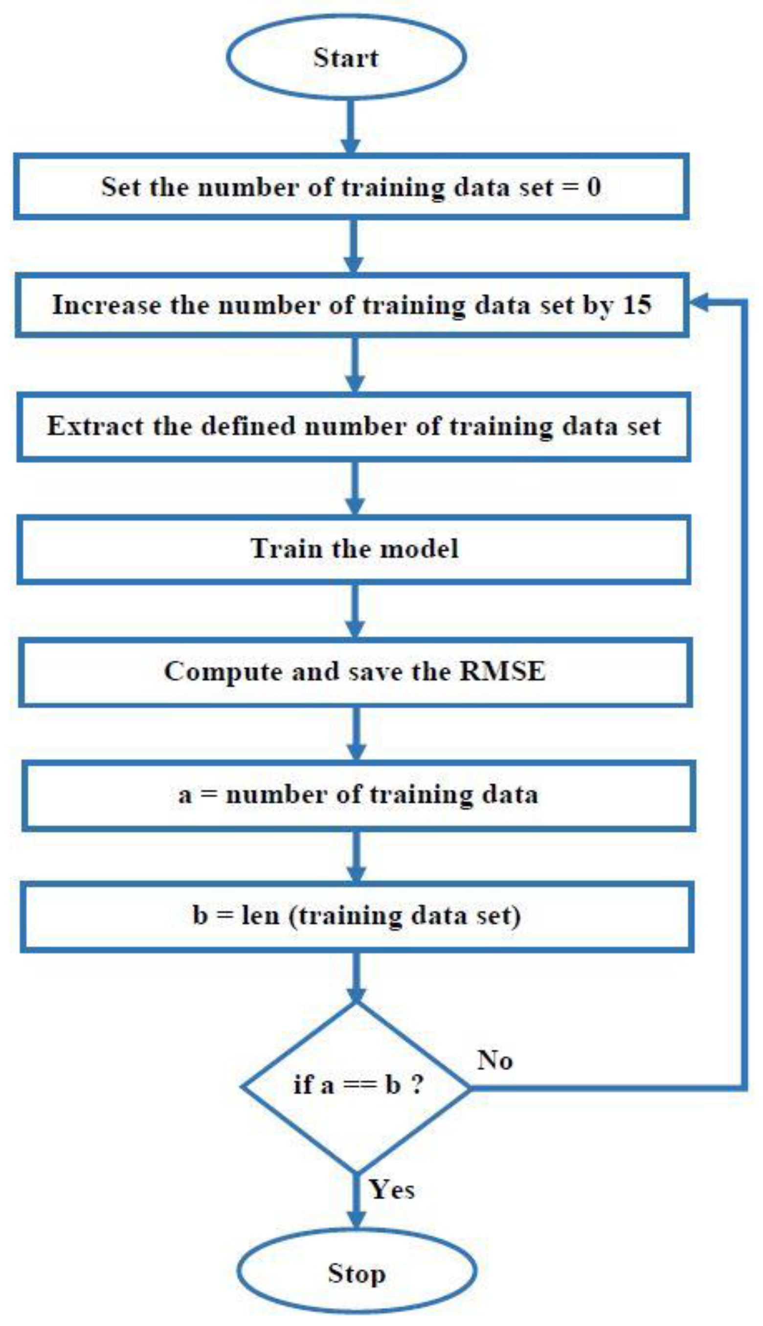
A set of data can most often, but not always, be observed in terms of equally spaced time intervals and can thus be termed as time series data. Unlike other models that account for a temporally dependent structure in the data, the presented model treats the forecasting problem as a curve-fitting exercise. Since these data are a function of time, while modeling, it is assumed that the factors affecting these data are a function of time as well and are not dealt with separately. As this model does not account for temporal dependencies and the output of the model is strictly a function of time, one of the methods to optimize the model is to experiment with the training datasets. This suggests the following question: What training dataset size does the model require for the short-term forecasting of kinetic energy with the least margin error? Hence, an optimization model was created to answer this question and is shown in Figure 3. At first, the available data (i.e., 525,604 samples) were divided into training and test sets, where the test set contained the last 30 min of data (arranged in minute intervals), and the rest of the data were considered to belong to the training set. Then, with the help of the training dataset, the model predicts the kinetic energy for the next 30 min. The forecasted output and the test dataset are then used to compute the RMSE. The number of training sets was incremented by 15 and the aforementioned process was repeated continuously. The RMSE computed at each step was recorded and plotted against the number of training samples. In the end, the number of the samples with the lowest resulting value for RMSE was considered to be optimal.

2.3. Performance Evaluation and Validation

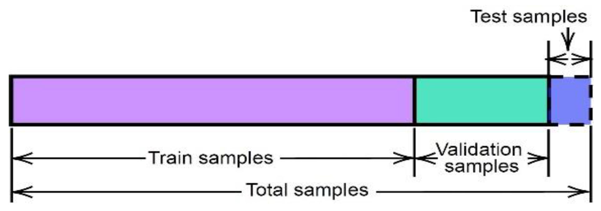
After developing a model, performance evaluation and validation are critical in research and development activities. In this study, a Bayesian model is used to forecast the time series data of kinetic energy within the INPS. The pre-processed data are firstly trained with ideal regression coefficients and an in-sample forecast is produced. In this process, a group of test samples is used for the validation of the results. The size of the test sample was considered to be 30 (i.e., 30 min), since this study is focused on forecasting for a short-term period. Similarly, the proportion of training and validation samples was considered to be 70/30. Figure 4 presents the distributions of the training, testing, and validation samples among the total samples. The forecasting technique used in this study was of an in-sample type. After analyzing the performance of the model and the nature of the kinetic energy, model validation was computed using popular measures like the mean absolute percentage error (MAPE), mean absolute error (MAE), root-mean-square error (RMSE), and mean absolute scaled error (MASE) as given in Equation (18). In Equation (18), yi and ŷi indicate the actual and forecasted values, ej is the error (i.e yiŷi) at the j-th iteration, and the training set is considered for time t (t = 1, 2, … T). A platform called EXPLORATORY is used for the performance evaluation and validation of the datasets [35]. EXPLORATORY uses R as the programming platform and provides the facility of data extraction, data wrangling, data analysis, data visualization, and so on via machine learning algorithms.
MAPE = 1 n i = 1 n | y i y ^ i y i | ,   MAE = 1 n i = 1 n | y i y ^ i | ,   RMSE = 1 n i = 1 n ( y i y ^ i ) 2   and   MASE = 1 j   0 j | e j | 1 T 1   t = 2 T | y i y i 1 |

3. Results

The main objective of this research paper was to analyze the time series data of kinetic energy and forecast short-term results that could be used for the estimation of power system performance indicators to ensure the secure operation of that system. To achieve this objective, the authors selected the case of the INPS, which interconnects the transmission systems of Norway, Sweden, and eastern Denmark. The respective TSOs have time series data of kinetic energy since 2015, which presents a great opportunity for performance estimation. Hence, the authors took the time series data (one sample per minute) of kinetic energy within the INPS for the whole year of 2019 and utilized the data for further investigation. The characteristics of the data can be visualized as per the box plots given in Figure 5. As shown in Figure 5a, the kinetic energy of the case study was found to be dependent on the weather, where it was comparatively high in winter and low in summer. Figure 5b,c present the weekly and daily characteristics of the kinetic energy, from which it may be observed that the amount of kinetic energy is above average during working hours and below average during non-working hours and holiday periods. Figure 6a,b gives the actual trend of the kinetic energy for the daily and annual period of 2019. A trend with the recorded maximum and minimum values of the kinetic energy can be observed. Overall, for the specific case study of the INPS, the nature of kinetic energy was found to be dependent on the working period and the weather.
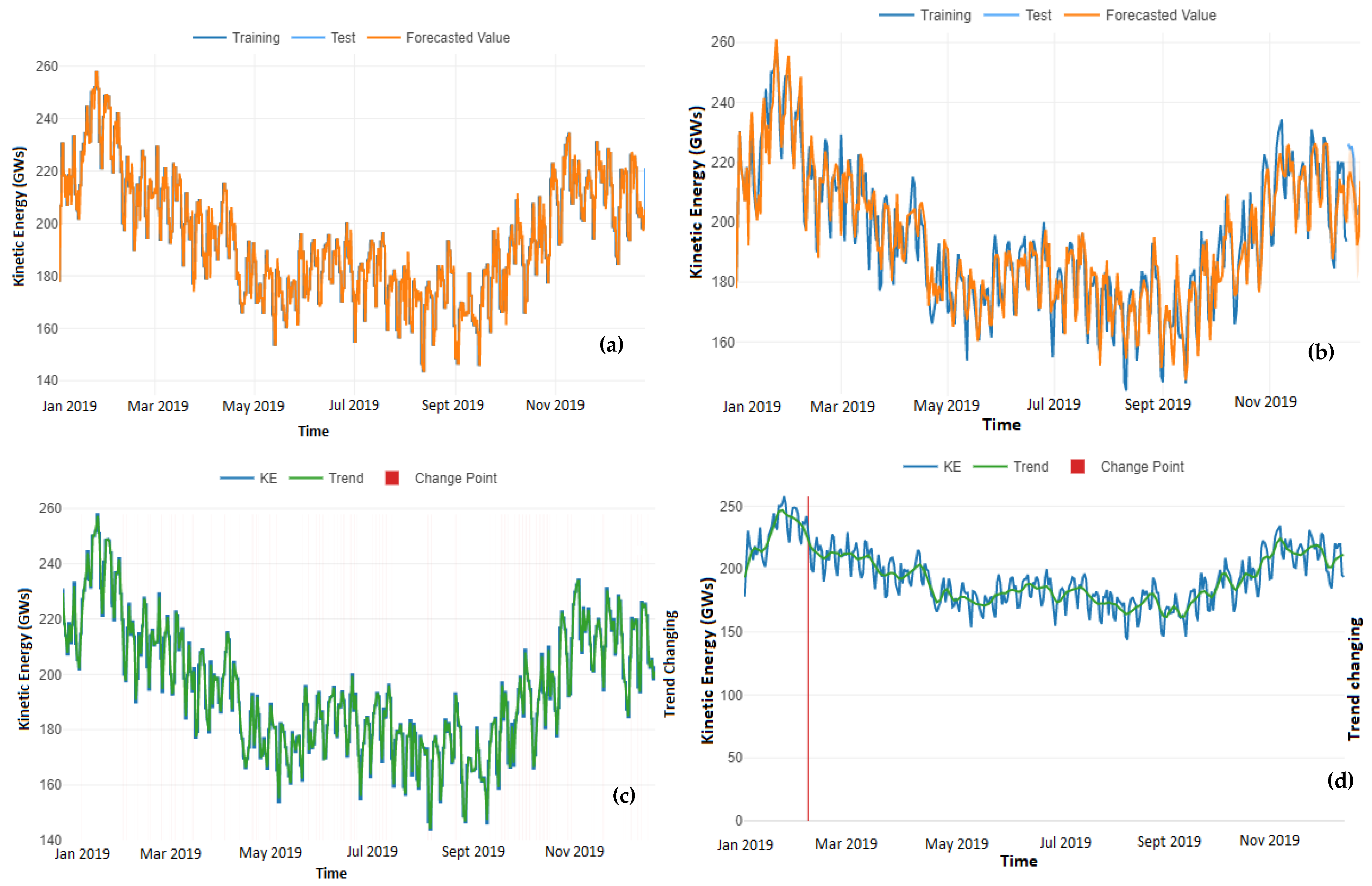
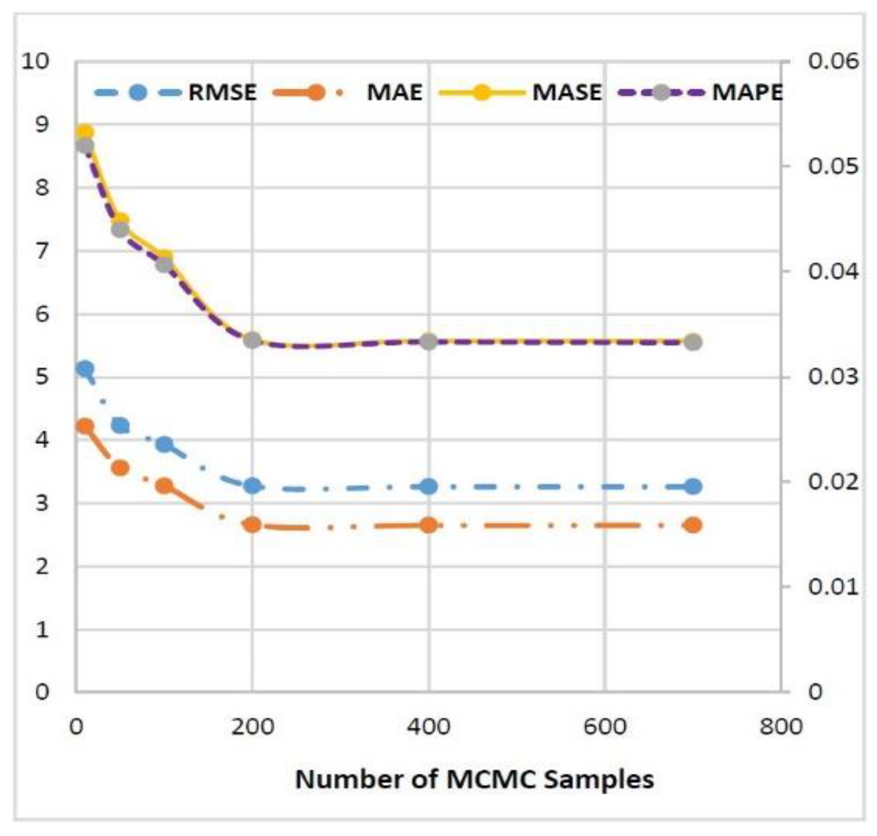
Figure 7 is focused on the characteristics of the forecasted data, along with the training and testing samples of kinetic energy. In this study, the kinetic energy was forecasted for 30 min. Figure 7a presents the nature of the training, testing, and the forecasted data obtained using the Bayesian model, whereas Figure 7c present the present trend of the kinetic energy and the changing patterns for the datasets. No changing trend points were identified that contributed to the trend variation of the kinetic energy when the Bayesian model is implemented. On the other hand, Figure 7b presents the nature of the training, testing, and the forecasted data for the ARIMA model, and Figure 7d presents the trend for the samples. The changing trend point was observed when the ARIMA model was implemented to forecast the data of kinetic energy within the INPS. Figure 8 shows a zoomed window for the last five hours that presents a clear comparison of the results for the proposed Bayesian model and the ARIMA model. After the short-term forecasting of the collected datasets, the results were used to validate accuracy and for future analysis. The values of RMSE, MAE, MAPE and MASE for the presented Bayesian model were calculated to be 4.67, 3.865, 0.048 and 8.15, which could be further improved by increasing the MCMC sampling. Figure 9 presents the performance metrics of the Bayesian model with different MCMC sampling values, and it is clearly shown that the optimum value is achieved with 200 MCMC samples. At this instant, the values of RMSE, MAE, MAPE, and MASE were identified to be 3.28, 2.67, 0.034, and 5.62. On the other hand, the values of the performance metrics for the ARIMA model were calculated to be 6.15, 4.680, 0.069, and 12.34. From the comparison of both models, the presented Bayesian model was found to be more accurate than the ARIMA model.
Similarly, Figure 10 presents the RMSE for a different number of training sets at which forecasting was computed for the next 30 min. The minimum RMSE (i.e., 1.54504) was obtained when 10,830 min of training samples was used. From this result, it is clear that a training data set of 10,830 min (or 180.5 h) is optimal to forecast the kinetic energy (for the specific case of INPS) for a short-term result (i.e., 30 min) with a value of 1.54504 for the RMSE.

4. Discussion and Conclusions

With the rapid development of new RESs, most countries are promoting these sources and interconnecting them into their power systems, since conventional power production necessitates the production greenhouse emissions and thus is not sustainable. At the current stage, most power systems are adopting such changes not only in the generation, but also regarding the transformation that occurs in transmission, distribution, and utilization because of the flexibility of EPC-based technologies. Because of this transformation, modern power systems are facing numerous issues. The major issues include maintaining proper frequency quality and an insufficient system rotational inertia within the power system to ensure operational security. In a conventional power system, the large proportion of synchronous generators acts as the source of inertia, which helps the overall system to maintain system frequency by providing inertial support during contingencies; however, unpredictable power sources with low inertia and flexible demand increase vulnerability to system instability in modern power systems since frequent power unbalance can create frequency deviations and this lead to system instability.
There are several power generators within a power system which must be synchronized and operated with the same frequency. During a power deviation event, if the deviation is comparatively high, then each individual machine tends to fluctuate around the centre of inertia (COI) and operate with a dissimilar frequency to other machines, which may result in system oscillation; however, the frequency of an individual machine close to the COI and some forms of inertial and damping forces attempt to maintain the synchronicity by pulling their frequencies toward the COI. If these forces become insufficient to recover synchronicity, a control mechanism must be applied to recover them, otherwise, the whole power system may undergo an unstable situation and system blackouts may even occur. The stability of a power system is directly dependent on the rate of change of frequency (RoCoF) and the nadir frequency, which are closely associated with system inertia. With an increasing frequency deviation and nadir frequency, an additional control mechanism must be introduced at the right time such that the system operates securely. Also, low system inertia decreases the critical fault clearing time (CCT), which means the minimum time to restore the system to an original stage is drastically decreasing in modern power systems. Hence, the estimation of system inertia, frequency, and/or nadir frequency is especially important for modern power systems.
Several research works have been conducted to estimate performance indicators such that power systems can be operated securely; however, most of them are focused on the measurement and estimation of frequency and nadir frequency. Some researchers have tried to estimate system inertia by taking the parameters from a power system during contingencies; however, one of the most complicated parts of estimation is that an inertial response cannot be distinguished by controlling units, and it is quite difficult to analyze dynamic performance in normal conditions. Forecasting system parameters such as frequency, nadir frequency, power generation, power consumption, and system inertia can be a good option, but this requires additional computational work with complex models and high response times for computation. A practical method that uses available resources is necessary to provide accurate and fast results to estimate system indicators.
This paper presents a practical method to estimate the dynamic characteristics of a power system by forecasting univariate time series data of kinetic energy. A Bayesian model is used to forecast the time series data of the kinetic energy, and a decomposable approach is used to analyze the characteristics of the dataset. From this study, it is found that the kinetic energy can be forecasted and analyzed using the Bayesian model with an acceptable accuracy limit and can be utilized in the estimation of the system inertia and the dynamic characteristics of a power system. Furthermore, the accuracy of the model can be improved by increasing the number of MCMC samples. In the considered case study, the optimized number of MCMC samples was found to be 200. A comparison of the results shows that the presented model is more accurate than an ARIMA model. For the specific data type in this study, a historic data quantity of 180.5 h was sufficient to forecast short-term results (i.e., 30 min) with a value of 1.54504 for the RMSE.

Author Contributions

Conceptualization, A.S. and F.G.-L.; methodology, A.S.; software, A.S. and B.G.; validation, F.G.-L.; formal analysis, A.S.; investigation, A.S. and B.G.; writing—original draft preparation, A.S.; writing—review and editing, All; supervision, F.G.-L. All authors have read and agreed to the published version of the manuscript.

Funding

There is no special funding to mention.

Institutional Review Board Statement

Not applicable.

Informed Consent Statement

Not applicable.

Data Availability Statement

The data are available upon request.

Acknowledgments

Ashish Shrestha is thankful to the Department of Electrical Engineering, Information Technology and Cybernetics, University of South-Eastern Norway, Porsgrunn, Norway, for the supports that he receives during his PhD. Also, the authors are thankful to the EXPLORATORY team, who made an extraordinary tool to analyze the time series data.

Conflicts of Interest

The authors declare no conflict of interest.

References

  1. Kerdphol, T.; Rahman, F.S.; Mitani, Y. Virtual inertia control application to enhance frequency stability of interconnected power systems with high renewable energy penetration. Energies 2018, 11, 981. [Google Scholar] [CrossRef] [Green Version]
  2. Kroposki, B.; Johnson, B.; Zhang, Y.; Gevorgian, V.; Denholm, P.; Hodge, B.-M.; Hannegan, B. Achieving a 100% renewable grid: Operating electric power systems with extremely high levels of variable renewable energy. IEEE Power Energy Mag. 2017, 15, 61–73. [Google Scholar] [CrossRef]
  3. Perez-Arriaga, I.J. Managing large scale penetration of intermittent renewables. In Proceedings of the MITEI Symposium on Managing Large-Scale Penetration of Intermittent Renewables, Cambridge, MA, USA, 20 April 2011; p. 2011. [Google Scholar]
  4. Khadka, N.; Paudel, R.; Adhikary, B.; Bista, A.; Sharma, S.; Shrestha, A. Transient Stability in Renewable Energy Penetrated Power Systems: A Review. In Proceedings of the RESSD 2020 International Conference on Role of Energy for Sustainable Social Development in ‘New Normal’ Era, Kathmandu, Nepal, 28–29 December 2020. [Google Scholar]
  5. Tuttelberg, K.; Kilter, J.; Wilson, D.; Uhlen, K. Estimation of power system inertia from ambient wide area measurements. IEEE Trans. Power Syst. 2018, 33, 7249–7257. [Google Scholar] [CrossRef] [Green Version]
  6. Zhang, Y.; Bank, J.; Wan, Y.-H.; Muljadi, E.; Corbus, D. Synchrophasor measurement-based wind plant inertia estimation. In Proceedings of the 2013 IEEE Green Technologies Conference (GreenTech), Denver, CO, USA, 4–5 April 2013; pp. 494–499. [Google Scholar]
  7. Fereidouni, A.; Susanto, J.; Mancarella, P.; Hong, N.; Smit, T.; Sharafi, D. Online Security Assessment of Low-Inertia Power Systems: A Real-Time Frequency Stability Tool for the Australian South-West Interconnected System. arXiv 2020, arXiv:2010.14016. [Google Scholar]
  8. Schiffer, J.; Aristidou, P.; Ortega, R. Online estimation of power system inertia using dynamic regressor extension and mixing. IEEE Trans. Power Syst. 2019, 34, 4993–5001. [Google Scholar] [CrossRef] [Green Version]
  9. Beltran, O.; Peña, R.; Segundo, J.; Esparza, A.; Muljadi, E.; Wenzhong, D. Inertia estimation of wind power plants based on the swing equation and phasor measurement units. Appl. Sci. 2018, 8, 2413. [Google Scholar] [CrossRef] [Green Version]
  10. Zografos, D.; Ghandhari, M.; Eriksson, R. Power system inertia estimation: Utilization of frequency and voltage response after a disturbance. Electr. Power Syst. Res. 2018, 161, 52–60. [Google Scholar] [CrossRef]
  11. Zografos, D. Power System Inertia Estimation and Frequency Response Assessment; KTH Royal Institute of Technology: Stockholm, Sweden, 2019. [Google Scholar]
  12. Heylen, E.; Strbac, G.; Teng, F. Challenges and opportunities of inertia estimation and forecasting in low-inertia power systems. arXiv 2020, arXiv:2008.12692. [Google Scholar]
  13. Allella, F.; Chiodo, E.; Giannuzzi, G.M.; Lauria, D.; Mottola, F. On-line estimation assessment of power systems inertia with high penetration of renewable generation. IEEE Access 2020, 8, 62689–62697. [Google Scholar] [CrossRef]
  14. Cancelo, J.R.; Espasa, A.; Grafe, R. Forecasting the electricity load from one day to one week ahead for the Spanish system operator. Int. J. Forecast. 2008, 24, 588–602. [Google Scholar] [CrossRef] [Green Version]
  15. Amaral, L.F.; Souza, R.C.; Stevenson, M. A smooth transition periodic autoregressive (STPAR) model for short-term load forecasting. Int. J. Forecast. 2008, 24, 603–615. [Google Scholar] [CrossRef]
  16. Taylor, J.W. An evaluation of methods for very short-term load forecasting using minute-by-minute British data. Int. J. Forecast. 2008, 24, 645–658. [Google Scholar] [CrossRef]
  17. Gonzalez-Longatt, F.; Acosta, M.; Chamorro, H.; Topic, D. Short-Term Kinetic Energy Forecast using a Structural Time Series Model: Study Case of Nordic Power System. In Proceedings of the 2020 International Conference on Smart Systems and Technologies (SST), Osijek, Croatia, 14–16 October 2020; pp. 173–178. [Google Scholar]
  18. Harvey, A.C.; Peters, S. Estimation procedures for structural time series models. J. Forecast. 1990, 9, 89–108. [Google Scholar] [CrossRef]
  19. Taylor, S.J.; Letham, B. Forecasting at scale. Am. Stat. 2018, 72, 37–45. [Google Scholar] [CrossRef]
  20. Novak, J.; McGarvie, S.; Garcia, B.E. A Bayesian model for forecasting hierarchically structured time series. arXiv 2017, arXiv:1711.04738. [Google Scholar]
  21. Vosseler, A.; Weber, E. Forecasting seasonal time series data: A Bayesian model averaging approach. Comput. Stat. 2018, 33, 1733–1765. [Google Scholar] [CrossRef]
  22. Zeng, Z.; Li, M. Bayesian median autoregression for robust time series forecasting. Int. J. Forecast. 2021, 37, 1000–1010. [Google Scholar] [CrossRef]
  23. Xiao, Q.; Chaoqin, C.; Li, Z. Time series prediction using dynamic Bayesian network. Optik 2017, 135, 98–103. [Google Scholar] [CrossRef]
  24. Rodriguez, A.; Puggioni, G. Mixed frequency models: Bayesian approaches to estimation and prediction. Int. J. Forecast. 2010, 26, 293–311. [Google Scholar] [CrossRef]
  25. Steel, M.F. Bayesian time series analysis. In Macroeconometrics and Time Series Analysis; Springer: Berlin, Germany, 2010; pp. 35–45. [Google Scholar]
  26. Ganics, G.; Odendahl, F. Bayesian VAR forecasts, survey information, and structural change in the euro area. Int. J. Forecast. 2021, 37, 971–999. [Google Scholar] [CrossRef]
  27. Thompson, P.A.; Miller, R.B. Sampling the future: A Bayesian approach to forecasting from univariate time series models. J. Bus. Econ. Stat. 1986, 4, 427–436. [Google Scholar]
  28. Zhang, A.Y.; Lu, M.; Kong, D.; Yang, J. Bayesian Time Series Forecasting with Change Point and Anomaly Detection. In Proceedings of the Sixth International Conference on Learning Representations, Vancouver, BC, Canada, 30 April–3 May 2018. [Google Scholar]
  29. Van der Heijden, M.; Velikova, M.; Lucas, P.J. Learning Bayesian networks for clinical time series analysis. J. Biomed. Inform. 2014, 48, 94–105. [Google Scholar] [CrossRef] [PubMed] [Green Version]
  30. Panagiotelis, A.; Smith, M. Bayesian density forecasting of intraday electricity prices using multivariate skew t distributions. Int. J. Forecast. 2008, 24, 710–727. [Google Scholar] [CrossRef]
  31. Carpenter, B.; Gelman, A.; Hoffman, M.D.; Lee, D.; Goodrich, B.; Betancourt, M.; Brubaker, M.A.; Guo, J.; Li, P.; Riddell, A. Stan: A probabilistic programming language. Grantee Submiss. 2017, 76, 1–32. [Google Scholar] [CrossRef] [Green Version]
  32. Nocedal, J.; Wright, S. Numerical Optimization; Springer Science & Business Media: Berlin, Germany, 2006. [Google Scholar]
  33. Neal, R.M. Slice sampling. Ann. Stat. 2003, 31, 705–741. [Google Scholar] [CrossRef]
  34. Nishio, M.; Arakawa, A. Performance of Hamiltonian Monte Carlo and No-U-Turn Sampler for estimating genetic parameters and breeding values. Genet. Sel. Evol. 2019, 51, 73. [Google Scholar] [CrossRef] [Green Version]
  35. Nishida, K. Introduction to Exploratory v6.0. Available online: https://exploratory.io/note/kanaugust/Online-Seminar-28-Introduction-to-Exploratory-v6-0-EdY3YOC2HC (accessed on 11 June 2020).
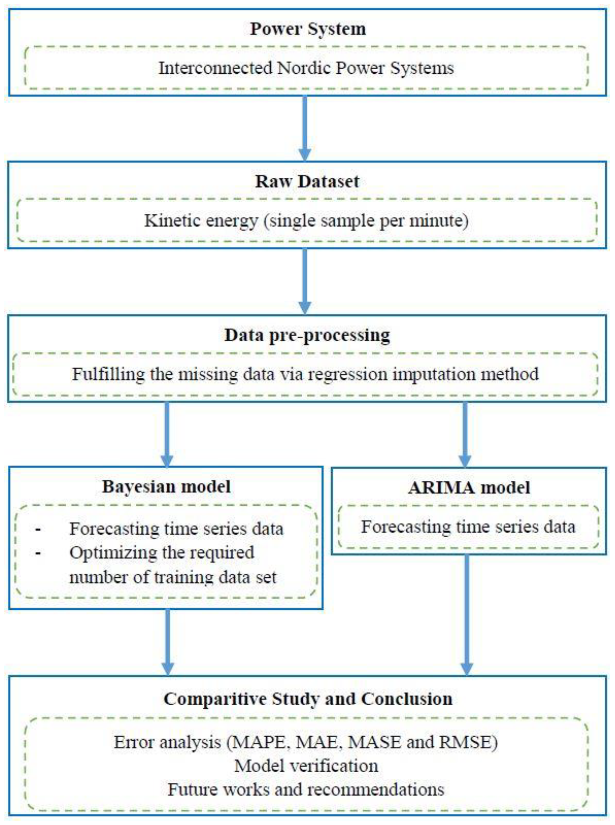
Figure 1. Adopted workflow.
Energies 14 03299 g001
Figure 2. Flow chart of the limited-memory Broyden–Fletcher–Goldfarb–Shanno (LM-BFGS) algorithm.
Energies 14 03299 g002
Figure 3. Flow chart of the optimization process.
Energies 14 03299 g003
Figure 4. Method of performance evaluation and validation.
Energies 14 03299 g004
Figure 5. Seasonal variations of KE: (a) annual, (b) weekly, and (c) daily.
Energies 14 03299 g005
Figure 6. Seasonal trend kinetic energy: (a) daily and (b) annual.
Energies 14 03299 g006
Figure 7. Results showing the nature of training, testing, and forecasted values by using (a) the Bayesian model and (b) ARIMA model. Similarly, (c,d) the trend and changing trend patterns for the Bayesian and ARIMA models are shown.
Energies 14 03299 g007
Figure 8. Zoomed window for the last five hours (a) for the Bayesian and (b) ARIMA models.
Energies 14 03299 g008
Figure 9. Effect of the Bayesian inference on the performance metrics.
Energies 14 03299 g009
Figure 10. RMSE values for different training sample number values for short-term forecasting.
Energies 14 03299 g010
Publisher’s Note: MDPI stays neutral with regard to jurisdictional claims in published maps and institutional affiliations.