Non-Destructive Quality Control of the Adhesive Rigid Timber-to-Concrete Connection in TCC Structures

Abstract

One of the limitations of using glued connections in practice is related to the need for connection quality control. Still, the need for the non-destructive quality control of finished products to determine the compliance of the developed structure with the designed one still exists. Considering the small amount of research on timber–concrete composites with glued connections, there is a lack of research on non-destructive methods for the quality control of rigid connections in timber–concrete composite structures. During the literature analysis, no information was found on the possibilities of testing the quality of the rigid timber-to-concrete connection. Therefore, two well-known methods—operational modal analysis and ultrasonic testing—were tested to verify the possibilities of applying these methods in determining defects in the rigid glued connection between the concrete and timber layers in the timber–concrete composite structures. A series of small-scale specimens produced by the stone chips method with and without artificially made defects in the timber-to-concrete adhesive connection was tested by both methods. Operational modal analysis shows significant changes in mode shape, frequency values, and spectral density diagrams. Despite the sufficiently large reflection of the ultrasonic signal on the timber and concrete boundary, the transmitted signal is sufficient to perform local ultrasonic tests for detecting defects in the adhesive connection. Thus, it is concluded that the principles of both methods can be applied in practice, and further research is needed to develop testing technology.

1. Introduction

Non-destructive testing methods provide an opportunity to evaluate the integrity of a material, component or system, and material properties and to identify and characterize damage without causing damage to the material being tested [1,2,3]. The methods provide effective ways of testing specimens for production quality control [4] as well as for monitoring the condition of structures during their operation [5,6,7]. Many different non-destructive testing methods are used in construction, each with its advantages and limitations. In construction, non-destructive testing methods, such as experimental test methods with static or dynamic load, impulse loads or vibrations as dynamic load, acoustic non-destructive testing methods, etc., are used to assess the condition of structures. The names of these methods usually refer to a particular scientific principle or equipment used to perform the test.

Static loading of structures is widely used for testing in laboratory conditions. For on-site assessment of the structure’s technical condition, this method is usually used only in cases where it is impossible to do otherwise because this method is time- and labor-intensive and sometimes even dangerous as it can cause the structure to collapse.

One of the most common ways to detect structural defects is by monitoring their dynamic parameters by loading the structures with the dynamic load. Some studies [8,9] demonstrate the effectiveness of non-destructive diagnostics with modal analysis for safe monitoring and damage assessment of structures such as concrete–steel composite beams with adhesive connections as well as laminated glass modular units. This method, experimental modal analysis (EMA), assumes that there is a known impact on the structure and the response of the structure to a specific impact. It is possible to determine the dynamic structure parameters by applying the transformation functions.

The impossibility of always evaluating all the effects of the surrounding environment on the structure and the limitations of the method, which are related to the dimensions of the inspected object, are the main reasons for the development of operational modal analysis (OMA). Operational modal analysis, also called “ambient modal analysis” or “data-only modal analysis”, is widely used in modal evaluations of large structures with environmental and service loads [10]. This method has several advantages over EMA [11,12,13]:

• OMA enables modal analysis without knowing and/or controlling the input excitation;
• Allows estimating the same modal parameters—mode shape of oscillations, natural frequency, and damping coefficient—as traditionally known methods;
• OMA belongs to the multi-input/multi-output (MIMO) method, which allows accurate estimation and repetition of mode shapes in space;
• Tests are more economical and quick to perform than EMA. The OMA method does not require additional equipment to excite the system, such as a vibrating platform or impact hammers for laboratory testing. When performing OMA tests, the input effect on the specimen can be random touching of the specimen in time and space, parallel to the measurement of vibration responses in several places. The excitation generated in this way is a good approximation of a multivariate white noise stochastic process.

It is hypothesized that by operational modal analysis, it is possible to determine the influence of the presence of defects in the adhesive rigid timber-to-concrete connection in the canopy on the modal structure parameters because studies show that the modal structure parameters are sensitive to structural damage [8,14,15,16]. Of course, the application of this method in the assessment of floor structures during operation is limited because, during operation, floors are especially exposed to external loads that change their dynamic calculation scheme.

Ultrasonic testing is one of the most widely used acoustic methods for detecting material defects and structural changes [17]. Ultrasonic waves have the property of propagating straight in a homogeneous medium. The transmitter sends an ultrasonic pulse into the material. When defects are encountered, the ultrasonic wave is partially reflected, and the receiver converts the ultrasonic oscillations into electrical oscillations and displays the information on the screen. This method’s shortcoming is that it can be applied locally because, in one measurement, information is obtained only about a specific area of the structure in which this measurement was made. There are studies on ultrasonic testing of concrete structures and timber structures. Still, there is a lack of information about the possibilities of using this method for the quality control of the timber-to-concrete adhesive connection in timber–concrete composite (TCC) structures.

A timber–concrete composite with a rigid adhesive connection between layers is a sustainable structure which can provide more efficient use of resources compared to TCC with the semi-rigid connection between layers, but the number of studies on this type of structure is limited. As of 2018, research on timber–concrete composite elements with a glued connection between concrete and timber layers was only around 2.5% [18]. As the rigid adhesive connection is the key to the TCC’s predictable behavior, it is essential to control the state of the connection to the designed one. There is a lack of research on the non-destructive methods of testing the quality of the rigid glued connection of timber–concrete composite structures. So, it is necessary to approbate non-destructive methods for the quality control of these connections to popularize in practice the use of timber–concrete composite structures with glued connections. Two well-known methods—operational modal analysis and ultrasonic testing—were experimentally tested to check the feasibility of applying these methods for the quality control of adhesive timber-to-concrete connections of TCC structures. As adhesive connections take a special position among timber-to-concrete connections in TCC structures and no analogous investigations have been carried out yet, this case study begins a series of investigations. The research presents the results of the testing of the principle itself. Further research to develop the testing technology is necessary.

2. Materials and Methods

Sixteen small-sized timber–concrete composite specimens with a length of 600 mm were made. One-half of the specimens have an artificial defect in the adhesive timber-to-concrete connection, and another has no man-made defect in the connection between composite layers. C24 strength class timber boards with a width of 95 mm and a height of 45 mm were used for the base of the specimens. The stone chips method [19] was used to produce timber–concrete composite specimens. The proposed production method includes gluing the granite chips with epoxy to the timber layer and placing a fresh fine-grained concrete layer after drying the adhesive layer. The granite chips with a fraction of 8–16 mm were glued with epoxy glue Sikadur-31CF. The thickness of used a uniform epoxy layer within the limits of 1–2 mm. Granite chip consumption is around 10.2 kg/m². After the glue had dried, a 20 mm thick layer of leveling compound for floors, Sakret BAM with strength class C20, was placed on the specimens in the molds. The overall specimen dimensions are shown in Figure 1a. For specimens with a defect in the connection, to ensure the complete absence of adhesion between the concrete and timber layers, the timber boards were covered with epoxy glue, but the stone chips were applied only to 60% of the surface of the specimen. After the glue layer dried, the rest of the specimen, equal to 40% of the specimen surface, without stone chips, was wrapped in a film, and then the chips were evenly placed on the film layer, with fresh concrete mass poured on top (Figure 1b). In this way, defects are modeled, which may arise, for example, due to non-compliance with the technological process of production and, according to calculations [20], may cause the structure to behave drastically different from the design. Specimen testing took place no earlier than 28 days after the concrete layer had been placed.

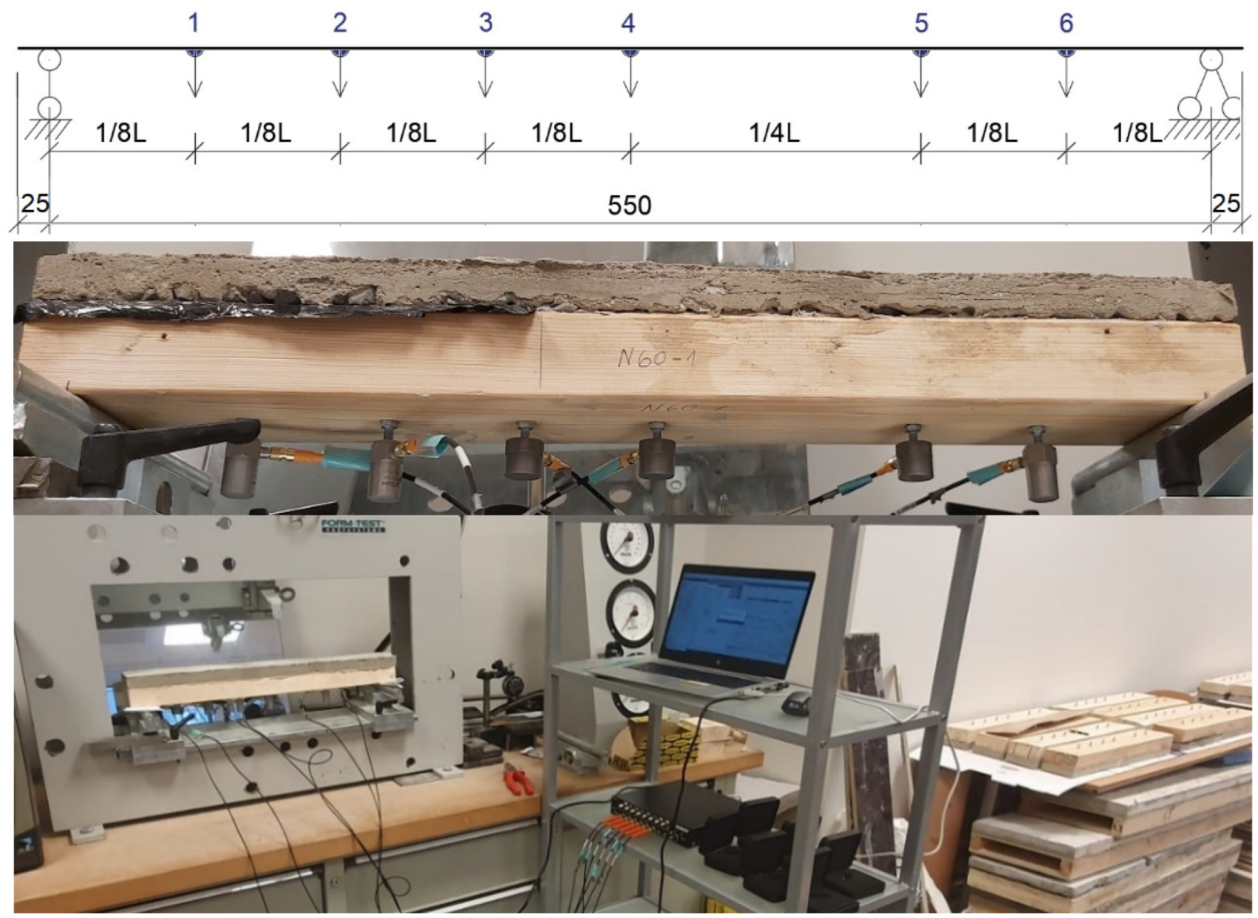
For modal analysis, a multi-input/multi-output method is provided by the use of six accelerometers, with which the structure’s response in the form of acceleration to white noise was measured. The specimen was simply supported, with a span of 550 mm, symmetrically to the ends of the specimen. The sensors were placed along the center line of the specimen according to the scheme shown in Figure 2. Two types of sensors from manufacturer Dytran Instruments, Inc. (Los Angeles, CA, USA) were available for the experiment: three sensors with low sensitivity of around 100 mV/EU (model 3312A2T) and three with high sensitivity of around 1000 mV/EU (model 3100D24), which were placed in positions 3, 4, and 5. In order to ensure fast, convenient and safe fastening of sensors to the specimens during the experiment, after the concrete layer had hardened, additional specimen preparation work was carried out. M5 bolts were glued with two-component epoxy glue to all the specimens according to the same scheme, creating a strong connection between the bolt head and the timber surface of the specimen.

All sensors are connected to a multi-channel high-precision dynamic signal analyzer—DT9857E manufactured by Data Translation (Marlborough, MA, USA), which receives sensor signals and sends measurement data to a computer. QuickDAQ computer software was used for data logging and initial data processing. Before taking measurements, all connected sensors were registered and configured in the program, specifying the sensitivity of each sensor as the number of millivolts per m/s² needed to scale the raw data. By recording the test measurements and evaluating the obtained frequency domain, a frequency of 4000 Hz was assumed as the maximum analyzed frequency for further measurements. To accurately record the signal, the sampling frequency was twice the maximum and equal to 8000 Hz, corresponding to an interval of 1/8000 = 0.000125 s.

For further data analysis, the measurements were transformed from the time domain to the frequency domain using a special mathematical function called the Fourier transform. If the signal changes over time can be observed in the time domain, then the frequency domain makes it possible to estimate how much signal there is in each specific frequency band, thus representing the qualitative behavior of the system. The obtained frequency spectrum allows evaluation of the ongoing process during the experiment. The fast and discrete Fourier transformation is based on dividing the measurements in the time domain into small blocks with a length of one block of T seconds and the further transformation of each block to the frequency domain. Spectral lines are reflected in the spectrum with a certain resolution, which means the distance between the spectral lines equal to Δf = 1/T Hz. The transformation result of each block is centered on the frequency of the corresponding line.

A fast Fourier transformation (FFT) block size equal to 16384 points was adopted, which provides 16384/2 = 8192 spectral lines and, subject to the defined sampling frequency, 8000/16384 = 0.488 Hz high spectral resolution. Such a high resolution allows us to recognize of closely spaced peaks but does not excessively burden the data processing process and the data visibility. It was assumed that each record contains 25 data blocks, the length equal to the size of the FFT. Taking into account the adopted frequency resolution and the number of average values, the total duration of one record is 25 × (1/0.488) = 51.2 s. The view of the record from one sensor is shown in Figure 3.

Of greatest interest are the frequency responses up to 1000 Hz, where several first peak values are located, so a second-order Butterworth low-pass digital filter with a cut-off frequency of 1000 Hz was applied to the input channels, which provides a maximally wide passband from 0 to 1000 Hz, which attenuates the signal within the limit by only 3 dB, while signals with a higher frequency than the cut-off frequency are gradually reduced at a rate of 12 dB per octave [21].

After configuring the QuickDAQ program, data collection was performed for each specimen, which involves:

• Placing the specimen on the supports and fixing the sensors.
• Excitation of white noise at random with time and space touches on the upper surface of the specimen along its entire length.
• Parallel to step 2, recording the response signal of the specimen.
• Repeating the measurements three more times.

The QuickDAQ program with the built-in FFT Analyser interface, which ensures the transition of the data recorded in each of the sensors to the frequency domain, is used only for the visualization and control of the processes occurring during the experiment. The ARTeMIS Modal program is used to further process and analyze the data obtained during the experiment. In the ARTeMIS program, the frequency domain decomposition (FDD) method, which is based on the frequency domain, is used to identify dynamic parameters, ensuring the process’s visibility and a user-friendly environment [22,23]. ARTeMIS provides an opportunity to perform data analysis, which is based simultaneously on the records of several sensors. For this purpose, the recorded raw data in the time domain are exported from the QuickDAQ program and imported into the ARTeMIS program. A Hanning window with 66% overlap was used for spectral density diagram estimation to reduce the possibility of spectral distortion and spectral leakage [24,25].

For all 16 specimens, the first three fundamental frequencies and mode shapes with their complexity were determined by automatic mode estimation, and singular values of spectral density diagrams were also evaluated. Two scales can be used for the analysis of the spectral density diagram—linear and semi-logarithmic. In the case of linear scaling, the spectral density diagram, which describes the distribution of signal energy in frequency components, represents the relationship between frequency and signal power in linear units. According to Parseval’s theorem, the signal power in the frequency domain can be obtained by integrating the acceleration, velocity, or displacement function in the time domain. In the case of a semi-logarithmic scale, changes in signal power are expressed in decibels (dB), which is a logarithmic quantity. The difference in signal power in decibels between two signals can be determined by Equation (1).

$$10\log \left(M_2{}^2/M_1{}^2\right)=20\log \left(M_2/M_1\right),$$

(1)

where M₁ and M₂ are the measured amplitude of the respective signal received by the sensors, for example acceleration, mm/s².

The semi-logarithmic scale makes it possible to cover a wider range of frequencies on a single graph and display a range of amplitudes intuitively. For example, a 128-fold reduction in signal magnitude can be represented as a reduction in signal power of only 21 dB.

In the case of modal analysis, it is necessary to ensure the same structure conditions to compare the structure’s current modal parameters with the initial ones. Considering that OMA application to monitoring during operation is difficult due to the type of use of the considered structure because TCC slabs are intended for use in floors, from which it follows that they are regularly exposed to short-term and quasi-permanent loads, which influences and changes the design scheme compared to the initially built structure’s reference state, the possibility of using the local non-destructive testing method, which does not depend on the design scheme, to control the quality of the TCC rigid connection during structure operation was tested.

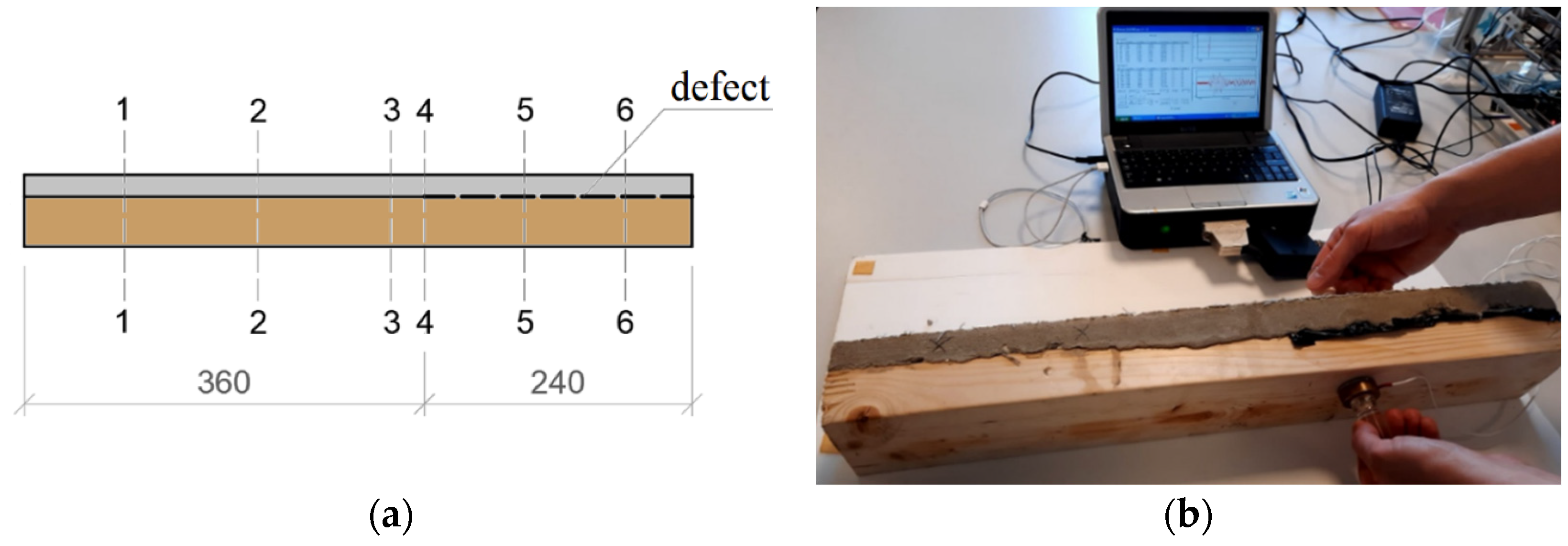
Since timber and concrete are different structural materials, laboratory testing of TCC specimens with a defect in the rigid connection has been carried out to clarify the expected results from local structural testing with ultrasound. A series of measurements were performed on four small-sized specimens with embedded artificial defects. Six measurements were made for each specimen. The measurement locations can be seen in Figure 4a. Measurements were made on the specimen part without defects (1–1 and 2–2) and with defects (5–5 and 6–6) as well as on the border (4–4) and near the boundaries (3–3) between the parts with and without defects.

The measurements were made with the experimental ultrasound apparatus and software developed at the Riga Technical University (Figure 4b) [26]. The transmitter and receiver consist of discs with piezo elements, and there are no signal suppressors in the model. Good adhesion between the surface of the specimen and the device is ensured by a special liquid. A single pulse with 100 kHz frequency characterized by a single period is sent. The measurement time of such a single pulse is approximately 1 millisecond. The speed of taking measurements was 30,000 SPS (number of samples per second), the resolution was 10 bits, and thus 0.001 × 30,000 × 210 = 30,720 points were used for the digitization of 1 millisecond of the measured signal. Still, due to the property of the ultrasound wave reflecting off the specimen’s edges, the recorded signal consists of many periods that gradually decay. The successful application of ultrasonic testing for adhesive connection quality control is based on the acoustic impedance difference in different materials. Acoustic impedance, Z, characterizes the material’s resistance level to the oscillations of ultrasonic waves. It can be calculated according to Equation (2).

$$Z=c·\rho ,$$

(2)

where Z is acoustic impedance; c is the sound speed, m/s; $\rho$ is material density, kg/m³.

The higher the material density, the higher the acoustic impedance value. When an ultrasound wave passes through one material and collides with the boundary of another material, part of the wave’s energy is reflected and part passes into the second material. How much energy is reflected is affected by the acoustic resistance, or impedance, of the two materials. When a wave passes through concrete or timber and encounters the air, almost 100% of the wave energy is reflected. This principle is the basis for the ultrasonic detection of defects involving air gaps. The reflection coefficient R as a percentage of the total wave energy can be calculated according to Equation (3) for any two materials.

$$R={\left(\frac{Z_2-Z_1}{Z_2+Z_1}\right)}^2·100\%,$$

(3)

where $Z_1, Z_2$ are the acoustic impedance values of the first and the second materials.

Table 1. Acoustic characteristics of materials.

	c, m/s	$\mathit{\rho }$, kg/m3	Z, kg/(sm2)
Air, 20 °C	344	1.2	412.8
Pine	2500	420	1,050,000.0
Concrete, C20	3700	2500	9,250,000.0

summarizes data for the acoustic impedance determination for pine, concrete, and air [27,28,29,30]. For pine timber, the speed of the sound wave is indicated in the direction in which the measurements were made, that is, in the radial direction. The acoustic impedance of the polypropylene film, which was used to ensure the defect in the timber-to-concrete connection, is comparable to the acoustic impedance of the timber material.

3. Results and Discussion

Other studies [8,9] had difficulty identifying differences in the first mode for specimens with and without defects, so that the specimens’ dynamic parameters, such as natural frequency, the mode shape, and its complexity, were defined for the first three modes. In addition to the automatically found, well-separated modes, whose frequencies are marked with circles in Figure 5, the diagram shows the so-called modal domain in light green and the modal coherence in light blue. The automatic peak search is based on the estimation of the so-called modal coherence. Modal coherence is a measure that is equal to 1 in the region where a particular mode dominates and is around the peak values. The upper part of the diagram corresponds to modal coherence 1, and the lower part of the diagram corresponds to 0. Between the peak values, the modes are mixed, and the modal coherence decreases significantly. The region dominated by a single mode is referred to as the modal domain. Within this, the frequency corresponding to the largest peak is chosen as the mode frequency. There are pronounced peaks in the spectral density diagram, which, according to the linear arrangement of the sensors, correspond to complex mode shapes. Therefore, it was concluded that measurements, even for elements working in one direction, are recommended to be carried out by placing the sensors spatially in two dimensions (for example, along the perimeter of the specimen) instead of linearly (i.e., only along the length of the specimen).

Figure 6a summarizes the average values of the frequencies of the first three modes. The first mode obtained based on experiment data was characterized by a high damping coefficient, which indicates noise. That is why comparing the first modes for specimens with and without artificial defects in the connection between composite layers was not made. It was concluded that even for elements working in one direction, it is important to place the sensors not linearly but two-dimensionally. The degree of reliability of the frequency values of the second and third modes was high. The noticeable difference between the specimens with and without defects is the frequency of the second mode. For specimens with a defect, it is higher than about 32%. No obvious difference is formed in the second mode shape, which is characterized by two waves at the considered type of artificial defect, which occupies almost half of the length of the specimen. By contrast, a significant change in the third mode shape was found for specimens with a defect in the timber-to-concrete connection. The modal assurance criterion, or MAC, which is a statistical measure used to compare the modes’ shapes, is equal to 0.55 for the third mode shape. This criterion is sensitive to large differences and relatively insensitive to minor differences in mode shapes. The closer the value of this criterion is to 1, the greater the coincidence of mode shapes. The normalized third mode shapes for all 16 specimens are summarized in Figure 6b. The defect-free specimens have a symmetric mode shape with three half-waves with a peak at the middle sensor location. For specimens with a defect, the mode shape remains asymmetric. The maximum is reached in the first half-wave on the side of the defect.

Changes can also be observed in the spectral density diagrams. If the third mode frequency, around 600 Hz for specimens without a defect, is dominant, then a low-level excitation can be observed at the third mode frequency for specimens with the defect. An increase in the value of the second mode frequency and the corresponding signal strength (at about 340 Hz) is observed for the specimens with defects (Figure 7).

Thus, the differences found in the modal analysis between the specimen series allow stating that damage in the rigid connection between the concrete and timber layers affects the responses and dynamic parameters of the TCC specimens. Therefore, under certain conditions, it is possible to effectively use operational modal analysis for assessing the quality of the timber-to-concrete connection and the presence of defects in TCC structures. The considered method allows non-destructive quality testing on a global scale, which can be especially relevant in high-volume production with large-sized structures when local inspection methods for defects would be time-consuming. By creating one reference structure that local inspection methods can test, the results of its modal analysis can be used as a reference for the other structures.

As a result of laboratory experiments, the possibility of successfully applying ultrasound testing for local quality control of a timber–concrete composite rigid adhesive connection was confirmed. Despite a sufficiently high reflection coefficient of ultrasonic wave energy between concrete and timber, which, according to calculations, is up to 64%, around 36% of the wave energy transferred to the second material is enough for ultrasound testing (Figure 8a). The data of six measurements for one of the specimens, as a time dependence of the relative amplitude of the measured signal, are summarized in Figure 8b). The physical significance of this value is related to the quality of the connection, and with its changes, it can judge the quality of the adhesive connection between timber–concrete composite layers.

Through a specimen part without a defect, far from the boundary where the defect starts, the ultrasonic signal passing through the specimen is strong and characterized by a large amplitude. Approaching the boundary with a defect, the maximum amplitude of the measured signal gradually decreases. On the other hand, in a place where a defect is pronounced and there is no nearby place without a defect, the ultrasound signal does not pass through the connection of the two materials. The signal amplitude value does not reach 10% of the maximum amplitude value at the signal transmission location without a defect. This amplitude value is mainly composed of the signal that spreads over the entire specimen and reflects from its edges and strays because the length of the specimen is not infinite. For larger specimen sizes, this amplitude percentage is even lower.

Ultrasonic testing can be used both to check the quality of manufactured elements to obtain a reference sample with which other elements can be compared and to detect technological defects in structures that were already revealed during operation. It is recommended to create a measurement grid for testing structures. Ultrasonic testing makes it possible to find defects with a diameter of 100 mm [31], but such size defects do not always have major engineering importance. Grid intersection points where measurements are made should be placed to match the size of the defects that significantly affect the behavior of the structure. If a point with drastically different measurement results is found, an additional finer measurement grid should be created around this measurement point to determine the defect’s contour.

Although using ultrasonic testing for the local detection of defects, as shown by the experiment, is possible, this method also has drawbacks. Firstly, similar to concrete structures [31], determining internal defects and their size requires well-qualified personnel with prior experience in interpreting ultrasonic testing results. In order to correctly decide on the size of the initial measurement grid, it is necessary to carry out an additional investigation to determine what size defects have a significant effect on the behavior of the structure. Although the time of one measurement is short (measurement time is only about 1 ms), the determination of the defect contour can be a time-consuming process due to the large number of measurements and the necessary preparatory work. Inspection of in-service structures is associated with the need to remove the floor finishing to gain access to the structural element, and in the case of direct transmission ultrasonic testing, access to the structure is required from both sides. Additional studies are necessary to provide some general rules for the number of measuring spots, time, prices, etc.

4. Conclusions

The possibility of using two non-destructive methods—operational modal analysis and ultrasonic testing—for the quality control of the adhesive rigid timber-to-concrete connection in timber–concrete composite structures was checked. Large-sized defects in the rigid timber-to-concrete connection impact the dynamic parameters of the timber–concrete composite structure, indicating the possibility of using modal analysis for non-destructive quality inspection purposes. The possibility of using operational modal analysis for the assessment of the quality of the adhesive connection between composite layers on a global level of structural timber–concrete composite members was approved and recognized as effective. Such significant differences between the timber–concrete composite specimens with and without artificial defects in the connection were determined within the experiments:

• Change in the third mode shape (the statistical measure used to compare the modes’ shapes—MAC = 0.55).
• Changes in frequency values for individual modes, reaching up to 32%.
• Changes in spectral density diagram as a signal power in individual modes.

A possible solution to the problem of timber–concrete composite adhesive connection quality control was proposed. The possibility of using ultrasonic testing has been approved and recognized as a perspective for local quality control of adhesive connection made by the stone chips method in timber–concrete composite structures. As a result of the experiment, it was obtained that:

• Despite the almost 10-fold difference in the acoustic impedances of concrete material and timber in the radial direction, 36% of the energy from the ultrasonic wave passing from one material to the other is sufficient to analyze the quality of the timber–concrete connection successfully.
• If the maximum amplitude of the measured signal at a high-quality adhesive connection is assumed to be 100%, then this value gradually decreases to 30–60% in the vicinity of the defect. In the case of a large and continuous defect, the measured signal corresponds to noise, and its maximum amplitude is below 10%.

The possibility of using the principle of OMA and ultrasonic testing for adhesive connections between composite layers as quality control in TTC structures has been verified. Further research is needed to develop the testing technology of the discussed methods.