Abstract
Accurate information about the available standing biomass on pastures is critical for the adequate management of grazing and its promotion to farmers. In this paper, machine learning models are developed to predict available biomass expressed as compressed sward height (CSH) from readily accessible meteorological, optical (Sentinel-2) and radar satellite data (Sentinel-1). This study assumed that combining heterogeneous data sources, data transformations and machine learning methods would improve the robustness and the accuracy of the developed models. A total of 72,795 records of CSH with a spatial positioning, collected in 2018 and 2019, were used and aggregated according to a pixel-like pattern. The resulting dataset was split into a training one with 11,625 pixellated records and an independent validation one with 4952 pixellated records. The models were trained with a 19-fold cross-validation. A wide range of performances was observed (with mean root mean square error (RMSE) of cross-validation ranging from 22.84 mm of CSH to infinite-like values), and the four best-performing models were a cubist, a glmnet, a neural network and a random forest. These models had an RMSE of independent validation lower than 20 mm of CSH at the pixel-level. To simulate the behavior of the model in a decision support system, performances at the paddock level were also studied. These were computed according to two scenarios: either the predictions were made at a sub-parcel level and then aggregated, or the data were aggregated at the parcel level and the predictions were made for these aggregated data. The results obtained in this study were more accurate than those found in the literature concerning pasture budgeting and grassland biomass evaluation. The training of the 124 models resulting from the described framework was part of the realization of a decision support system to help farmers in their daily decision making.
1. Introduction
Grazed pasturelands play multiple roles in agroecosystems that can benefit the sustainability of ruminant-based agriculture. This includes lower feeding costs [], higher animal welfare and lower occurrence of lameness and mastitis, and increased milk quality compared to indoor feeding []. However, despite these advantages, Walloon intensive dairy farmers increasingly turn away from grazing. This is because of the higher difficulty of managing grazed pastures as their main feeding method, especially with a decreasing workforce available on the farm and increases in herd sizes []. Indeed, due to the high variability of plant growth with weather conditions, grazing management requires a frequent assessment of the standing biomass available for animals to feed on. Tools like decision support systems (DSS) could ease this management from the farmer’s perspective by providing an assessment of the standing biomass without having to travel to the pasture. Such a DSS, based on the simulation of the behavior of a dairy farm practicing rotational grazing, was for example developed by Cros et al. [] and Amalero et al. [] to help farmers plan their activities. Other examples of DSS, like Pasture Growth Simulation Using Smalltalk (PGSUS) [,] and PastureBase Ireland integrating the Moorepark St Gilles grass growth model (MostGG) [], focus on the assessment of available forage in pastures. Both tools rely on reference field measurements used as inputs in mechanistic models. The reference measurement method consists of the cutting and drying of forage samples to get the actual dry biomass per area unit. This procedure was developed for researchers and is time-consuming, destructive, expensive and never applied by farmers. Moreover, the limited number of samples that can be taken strongly reduces the possibility of assessing the spatial variability of the pastoral resource. Objectives other than biomass might also be included in the DSS, such as leaf area index (LAI), real height or visual correspondence to standards.
Several alternatives to this reference measurement have been proposed, such as the indirect estimation of standing biomass [,,] via the measurement of compressed sward height (CSH) using a rising platemeter (RPM). The CSH readings can be converted into biomass with varying levels of accuracy, depending on the structure of the assessed vegetation []. While this method can provide a high number of estimates and also spatialize the data if combined with a GPS sensor [], it requires time to perform the measurement on the pastures. It also requires consideration of the sampling pattern to capture the spatial variability of height on a given pasture, MacAdam and Hunt [] recommends a “lazy W” sampling pattern while Gargiulo et al. [] shows that for a homogeneous pasture, the impact of the sampling pattern is negligible. In addition, no consensus exists on which part of the biomass to consider. The CSH measurement implicitly considers all standing biomass, while some scientists, like Wang et al. [], advise considering biomass above 1 cm. Others, like Hakl et al. [] and Walloon farm advisers, use a threshold of 4 cm, while Crémer [] and Nakagami [] bound the limit to 5 cm. Other methods to assess standing biomass include the response of the sward canopy to ultra-sonic [,,] or electric [,] signals, ground-level photography analysis []. All the methods cited previously require attention to be paid to the size, number and repartition of the sampling spots [] in order to minimize sampling error. Aside from these ground-based methods, the estimation of standing biomass has also been explored through remote sensing from either satellite or airborne platforms (e.g., [,,]). This offers already-spatialized data and reduces the risk of sampling bias. However, other constraints might appear, such as computation power requirements and the sensitivity of unmanned aerial vehicles to flight autonomy, weather and regulatory constraints. In the context of the current study, these constraints, together with the time-consuming aspect of acquiring data with unmanned aerial vehicles (UAV) led to the choice of not using this technology. However, it is worth mentioning that UAV based systems are at the core of current researches establishing relationships between the biomass and remote sensed data like digital surface/elevation models derived from aerial pictures (using structure from motion), LiDAR pointclouds acquisition and treatment, and spectral vegetation indices data [,,].
All these methods are part of a set of recent technological advancements that may help grazing management to embrace the smart farming approaches relevant to this sector [], provided their adequate integration in DSS and a good level of acceptance by farmers. The latter requires DSS to be based on information routinely available at a large scale and at minimal cost. Moreover, it must be possible to improve the DSS in an iterative and interactive process [].
In order to address the challenge of providing a tool offering a rapid estimation of pasture biomass under the above-mentioned constraints, the current study developed an analysis method to predict CSH measured on pasture using readily available meteorological data, space-borne synthetic-aperture radar (SAR) and optical imagery. Indeed, despite CSH being an indirect measurement of biomass, RPM has been widely used and benefits from widespread acceptance among farmers and pasture scientists (e.g., [,,]). Meteorological data have the advantage of being routinely available at the Walloon scale (i.e., for all the Southern part of Belgium which is the area of interest in this study) and provide insight into the key drivers of growth dynamics for various types of pasture plants growth dynamics [,,]. Such models are at the heart of most DSS (e.g., STICS [] and MostGG []).
Concerning the space-borne remote sensing data, a choice was made between all the existing optical and SAR sensors according to their spatial, temporal and spectral resolution, as well as their cost. The Sentinel-1 (S-1) and Sentinel-2 (S-2) constellations were chosen. S-1 was used for mowing event detection [], LAI and above ground biomass estimation [], or to detect meadow phenology []. S-2 mission was used for biomass estimation [,] or monitoring [,] or for LAI retrieval []. Some studies predicting standing biomass in grasslands have already included analysis of both S-1 and S-2 data [,]. However, they did not encompass any transformation of those signals, which might enhance some properties, such as how NDVI highlights the presence of chlorophyll in the vegetation. Nor did they test a wide range of machine learning (ML) methods that could catch different parts of the information. The methods appearing most frequently in these studies are multiple linear regression (lm), neural networks with or without recurrent layers, random forests (rf) and cubist, alone or together (e.g., rf and lm were used to predict the quantity and quality of grass swards in Alves et al. []). This study encompasses multiple variable transformations and ML methods (amidst the wide range of methods highlighted in Fernández-Delgado et al. [] and in García et al. []) with the objective of extracting more information on those signals. The framework described in this study aims to predict biomass in Walloon pastures through the CSH proxy using more than 100 different ML models, in order to provide a tool offering a rapid estimation of pasture biomass on the basis of readily available meteorological data, SAR and optical imagery.
2. Materials and Methods
The structure of this section follows the workflow presented in Figure 1. The main steps are the following: data acquisition and pre-processing, data fusion to a grid, separation of training and validation datasets, selection of the most informative variables, model training and validation. The processing framework was made in R v3.6.2 using Rstudio IDE v1.2.5033 [,]. The framework can be summarised according to the following equation: .
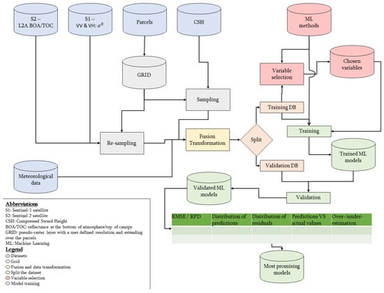
Figure 1.
Framework developed in the study to process Sentinel-1, Sentinel-2 and meteorological data to predict standing biomass in grazed pastures. The first steps are the pre-treatment and the (re-)sampling of the different dataset according to the same reference grid. Then the datasets are merged to get a tabular dataset. Transformations of the variables are then computed. Afterwards, machine learning models are trained and validated on distinct parts of the dataset. Based on the results of the validation, the most promising models are determined.
2.1. Study Area
Data were acquired over three farming areas in the southern region of Belgium, as shown in Figure 2, during two grazing seasons: from 5 May to 28 October 2018 and from 23 April to 20 September 2019. The three farms used rotational grazing of dairy cows. The first (Farm A in Figure 2) was an experimental farm located in the Condroz region. The second (Farm C in Figure 2) was a commercial farm located in the Famenne region. The third (Farm B in Figure 2) was also a commercial farm located in the Ardenne region. All the monitored grasslands were permanent multispecific grasslands.
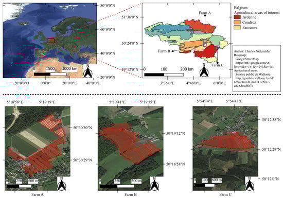
Figure 2.
Location the studied farms in the agricultural areas of Belgium and their grazing parcels.
2.2. Datasets
Compressed sward height
A total of 72,975 CSH records were acquired approximately weekly during the grazing seasons of 2018 on Farm A (N = 13,753) and Farm C (N = 9309), and 2019 on Farm A (N = 28,497) and Farm B (N = 21,416), using a Jenquip EC20G rising platemeter (NZ Agriworks Ltd t/a Jenquip, New Zealand). The relationship between CSH and time was integrated by considering two variables: the number of the month of the year (e.g., 1 for January) and the day of the year (e.g., 1 for 01/01).
Meteorological data
The meteorological data used came from the meteorological station located on the experimental farm. It consisted of the daily rainfall and the degree-day-18 (DD_18): , where and are the minimum and maximum temperature of the day. This formulation of the degree-day variables is introduced in studies like the ones of Moot et al. [] and Balocchi et al. []. In some cases, the minimum and maximum temperatures may have upper and lower threshold whose value depends on various factors including the ability of the plant to take water [], family and photosynthetic pathways (see the sensitivity of the Rubisco to temperature in Salvucci et al. [] and Greco et al. []). Given that the pastures are multispecific, it was chosen to ignore the threshold on minimum and maximum temperatures and the base temperature of 18 C was considered. In order to take the historical succession of meteorological events into account, the meteorological data were used in a cumulative way: the precipitation and the degree-day-18 were summed over periods of 3, 7 and 15 days and a mean of both variables since the last CSH measurement was also computed. Eight meteorological variables were thus considered in this study.
Sentinel-1 data
The S-1 mission offers SAR data in the C band (C-SAR) with a mode-dependent spatial resolution of roughly 5m and a revisit frequency of approximately three days over the studied area. It also has the advantage of providing data even in cloudy or night-time conditions. The S-1 C-SAR data were acquired as level-1 GRD products with VV+VH dual polarisation from the Copernicus Hub [,] through the use of a dedicated R package: getSpatialData v0.0.4 []. The pre-processing was done in accordance with the standardized framework described by Filipponi [,], based on the s1tbx toolbox [] from SNAP software v7.0.0. This gave products of roughly 5 m of spatial resolution, and consisted of:
- applying a precise orbit file: the real and precise orbit file was computed after the passage and is thus retrieved online to correct satellite position and velocity in the metadata;
- removing thermal noise;
- removing border noise: the artefacts at the image border were removed with the following two parameters: “borderLimit = 500” and “trimThreshold = 50”;
- calibrating SAR backscatter: place to choose the output between , and . The second index is related to the first through the cosine of the reflection angle: , with r being the reflection angle. The third one is described by equation: where represents the surface perpendicular to the beam, reflecting the totality of the power of the signal in an isotropic way and the surface of the pixel in radar geometry []. As recommended by Rudant and Frison [], only was considered in this study because is more suited for punctual targets and for dense forests;
- speckle filtering: the noise coming from the interference of reflected waves was removed with a ‘Refined Lee filter’ with a filter size of 3x3.
- terrain correction: the correction was made using the Shuttle Radar Topography mission data (SRTM 3sec);
- converting to decibel.
The S-1 data were represented in the dataset through two variables: of VV and VH channels.
Sentinel-2 data
The S-2 mission was chosen for its 13 optical bands, including the three in the red-edge spectral region. The resolution is band-dependent and is either 10 m, 20 m or 60 m with a revisit frequency of approximately three days over the studied area. The S-2 data were acquired as L2A-BOA/TOC (Level 2A corresponds to the reflectance at the bottom of the atmosphere or top of canopy) products from the Copernicus Hub [,] through the use of a dedicated R package: sen2r v1.3.3 []. Some tiles were only available as L1C-TOA products. The pre-processing to transform them into L2A-BOA/TOC tiles was done with the Sen2Cor toolbox [] and managed by the sen2r package. The main steps behind this transformation are precisely described in Mueller-Wilm [] and are summarised as:
- scene classification based on band and band ratio values comparison to threshold into 12 classes: 0—No Data; 1—Saturated or defective; 2—Dark area pixels; 3—Shadows of cloud; 4—Vegetation; 5—Not vegetated; 6—Water; 7—Unclassified; 8—Cloud medium probability; 9—Cloud high probability; 10—Thin cirrus; 11—Snow;
- atmospheric correction, consisting of: retrieving the aerosol optical thickness and water vapor, removing the cirrus and retrieving the impact of terrain to get BOA reflectance. It was chosen to ignore the DEM impact;
- product formatting into JPEG2000.
Another processing step involved the resampling of the bands at the same resolution and the fusion of the tiles per acquisition date. The sen2r package managed gdal v 3.0.2 [] for both operations. The resampling resolution was set to 10 m which was the smallest resolution of S-2 images. The scene classification was also recorded. In order to avoid major bias in reflectance measured, only tiles with less than 75% of clouds signaled in the metadata were downloaded and processed. The S-2 data were represented into 12 variables in the dataset (bands 1 to 12 without bands 9 and 10 and the scene classification layer). The first band was included although it is supposed to be related only to atmospheric correction. Its integration in the scope of studied variables aimed at detecting potential artifacts related to the S2 pre-treatment.
2.3. Grid
A sub-division of the studied area was performed, as done by Higgins et al. [] and Lugassi et al. []. In Ruelle abd Delaby [] and Ruelle et al. [], a grid with a resolution of 2 m was the best compromise between precision and speed of computation. Here a resolution of 10 m was chosen, representing a compromise between the spatial resolution of satellite images (it corresponded to the highest resolution of S-2 images) and the conservation of the variability of the CSH dataset.
The CSH records were first attributed to a pixel (i.e., a square unit of the grid) and when there was more than one record for a pixel, the CSH median value was considered. The S-1 and S-2 data were resampled using the same method (called “bilinear”): the pixel of the satellite image containing the center of the grid pixel was identified, then the four nearest satellite pixels were also identified, and a median value of these four neighboring values were allocated to the grid pixel.
The resampling was made independently for the different datasets in order to offer some modularity in the analysis. The R packages used for those operations were: data.table v1.12.8 [] and dplyr v0.8.3 [] which allowed different management of the data frames; sf v0.8-0 [], sp v1.3-2 [,] and raster v3.0-7 [] which allowed computation over spatial data and future v1.16.0 [] and future.apply v1.4.0 [] which were used to make the computation on parallel mode.
2.4. Fusion and Data Transformation
The fusion part consisted of gathering all the information in a single dataset with all the variables as columns and records as rows. First the gathering of all the spatial datasets was done according to their date of acquisition and pixel on the grid. In the case of non-simultaneous acquisition, the nearest acquisition to the CSH measurement was chosen within a 10-day time window. The second part consisted of attributing the meteorological data. To each record was attributed the value of the corresponding date. The non-linear relationship between the explanatory variables and the CSH may not be handled by all ML methods. To bypass those possible restrictions, some data transformations were computed, with some scaling when needed, and also integrated into the workflow:
- meteorological data: square () and exponential () transformations were applied on the cumulative data to compute 16 transformed variables;
- S-1: the transformations applied on the 2 S-1 variables were: square (), exponential (), inverse () and hyperbolic tangent (). Eight transformed variables of the S-1 dataset were added to the dataset;
- S-2: the transformation applied on the reflectance variables were: square (), cube (), exponential (), inverse () and hyperbolic tangent (), square root (), logarithm of base 10 (). A total of 77 transformed variables of the S-2 dataset were included in the dataset
Besides these transformations applied to each variable independently, some calculations were made on pairs of variables. Indeed, spectral indices may emphasize some particular spectral signatures []. This was taken into account in this study by integrating the 138 non-redundant vegetation indices, computed on the basis of the S-2 bands according to the formulas on the website “the Index DataBase” [], IDB []. A total of 249 indices were in fact developed in this list, but a comparison of each index highlighted redundancies (same expression and different names). To avoid the introduction of meaningless collinearity in the dataset, only the first index in order of appearance in the list was used.
2.5. Split the Dataset
The total dataset had 16,577 records and 277 variables. Independence between the training and validation datasets was ensured by splitting the dataset at the farm level: Farms A and C were used to train the model, whilst Farm B was used to validate. The training dataset thus had 11,625 records and the validation dataset 4952 records.
Potential outliers were highlighted by calculating the global H distance (GH) of those records from the principal components explaining 99% of the data variability. The principal component analysis (PCA) was performed with the FactomineR R package v2.1 []. Records with a GH value above 3 were considered with caution and records with a GH value above 5 were considered potential outliers. However, no value was discarded.
2.6. Variable Selection
As some of the ML methods explored in this study do not handle collinearity between features well, like the generalized linear model and the other methods presented in Table 1, a variable selection process was firstly performed, composed of three steps: (1) score determination, (2) definition of breakpoints, and (3) variable selection.

Table 1.
Presentation of the machine learning algorithms explored during the training processes. The column ‘Abbreviation and references’ gathers the abbreviations used in the text, corresponding to the name of the method in caret R package, and some articles using the methods in related fields.
The working hypothesis was that the probability of selecting a relevant feature is higher if this one was considered as important by several ML algorithms. Thus, 12 models resilient to collinearity were developed based on the parametrisation presented in Table 2 on the standardized training set with a 19-fold cross-validation (CV). The final models had the lowest CV root mean square error (RMSEcv). Then, a variable importance ranking was established for each model through the use of a function of caret R package v6.0-85: VarImp() []. For each variable, the mean and median of their ranking in all models were computed. In order to penalize variables with a high variability of ranking between developed models, the statistical descriptors were standardized: the mean of the ranking of each variable was divided by its standard deviation () and its median by its interquartile range ().
Table 2.
Presentation of the machine learning algorithms explored in variable selection and training processes. The column ‘Abbreviation and references’ gathers the abbreviations used in the text, corresponding to the name of the method in caret R package, and some articles using the methods in related fields.
The variables were ordered according to their decreasing ranking score. Then, multiple linear regressions were trained iteratively: initially, the most informative variable was used, then the first and the second most informative, and so on until all variables were included. For each regression, adjusted R-squared () was computed, and its first derivative was calculated starting from the second value by subtracting the previous value from the actual. A rolling median filter with a window width of three records was applied to this first derivative values to smooth the signal. The negative values corresponded to the breakpoints. To prevent the occurrence of noise, only the first breakpoints were considered in this study. For each breakpoint considered, the variables having a higher ranking than that breakpoint were used to train models through a 19-fold cross-validation based on the acquisition dates of CSH. The variables with a lower ranking were not taken into account.
2.7. Model Training
The training phase consisted of a 19-fold cross-validation based on the acquisition dates of CSH on the standardized data. The selection of the best model was made according to the lowest RMSEcv value. For each breakpoint considered, 31 ML methods, including the 12 used in the variable selection process were explored, each resulting in one model. Although some models failed to converge towards a reasonably performant and finite solution within a decent timestep (one week), all models that managed to get a usable expression were kept for further validation and analysis.
2.8. Model Validation
The models that did not fail during the training process were tested on the independent validation dataset. The indicators observed were the RMSE of validation (RMSEv), the distribution of the validation predictions of CSH compared to the original distribution of CSH, the distribution of the residuals (computed as the predicted value minus the actual value) and the mean residual value per class of CSH with a class width of 5 mm of CSH. The limits of the sampling tool were 0 and 250 mm of CSH. Predicted values beyond these thresholds were brought back to the nearest class. This might have resulted in some flooring and ceiling effects in the representation of the prediction and the residuals. A perfect model would have a low RMSEv, show no difference between the distribution of the actual and the predicted CSH, have a centered distribution of residuals and show no relationship between residuals and actual CSH values.
The models developed and validated on the grid pixel basis described previously were also tested on datasets aggregated at the paddock-level for each acquisition date. Two combinations of aggregation and prediction were tested: either the prediction was made on the pixel and then averaged at the paddock level, or the data were averaged at the paddock level and then the prediction was computed. For the sake of completeness, the combination of prediction and aggregation was tested on both the training and the independent validation dataset. Only a summary of the residual prediction deviation () is presented in this paper.
3. Results
3.1. Description of the Datasets
The distribution of CSH from the pixellated and aggregated points of view is summarised for the calibration and validation dataset in Table 3, and the distribution for each day of acquisition in Figure 3. Those results showed that the CSH measurements were not normally distributed.
Table 3.
Summary of the compressed sward height [mm] of both training and validation datasets. The aggregated lines correspond to the mean compressed sward height (CSH) per parcel per acquisition date.
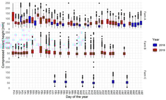
Figure 3.
Distribution of the CSH acquired during the farm walks on each recorded farming area following the day and the year of acquisition, the day of the year equals one being the first of January. The error bars (whiskers) extend from the upper/lower hinge of the box to the largest/smallest value within 1.5 times the interquartile range. The theoretical frequency of acquisition was one acquisition a week. The data were aggregated through all the parcels of each farm.
To reach 99% of cumulative percentage of variance, 41 principal components were considered. The distribution of GH for the training and validation records was summarised in Table 4. Records having a GH value higher than 5 represented less than 5% of each dataset: 150 (1 %) and 197 (4 %) in the training and validation sets, respectively. The higher number of outliers in the validation set is explained by the fact that the GH was calculated from the calibration set. Therefore, this means that a certain part of the variability in the data collected from Farm B was not totally covered. However, further investigations revealed that there was no apparent relationship between GH and CSH. It means that no subset of CSH occurs on a specific spot of the multidimensional space of components. A representation of the distribution of the GH per sampling date (data not shown) showed that there were more outliers for some recording dates. This could either reflect sampling issues or artifacts in the satellite data. It was chosen to keep these records, given that there is no certainty that these records are not linked to special meteorological events. Finally, one of the S-2 surface coverage, corresponding to the classification “shadow of cloud”, was represented only in the training dataset but no relationship between this classification and the GH stood out.
Table 4.
Summary of the global H distance (GH) of the training and validation datasets compared to the training dataset. Values above five are considered as potential outliers.
Figure 4 shows the two most informative axes of the PCA. These components together explained 54.9% of the variability of the explanatory variables. Some faint grouping effects of variables could be seen. A group was positively related to the first component, mainly made up of raw and transformed S-2 indices. Another group was related positively to both first and second components, mainly made of raw and transformed S-2 bands. A third group was related negatively to the first and positively to the second component, mainly made of raw and transformed S-2 bands. The large amount of S-2 related variables in the datasets hid the position of the other variables. They spread well over the two-dimensional space of Figure 4 although they seem to be more correlated with other components given the length of their arrows. Based on these results, the integration of multiple data sources seemed relevant as they bring different information. Moreover, the variables with a transformation spread well on the two-dimensional space of the two first components of the PCA although the variables with an inverse transformation seemed to be mainly negatively correlated with the second axis (data not shown). The integration of multiple variable transformations also appeared relevant. The proximity of some variables on the graph in Figure 4 implied a possibly non-negligible redundancy. Therefore, the selection of variables before the training of the models is critical.
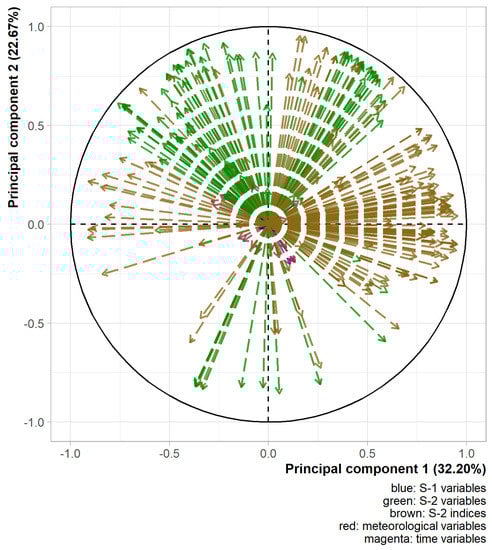
Figure 4.
Variable position on the two first principal components for the calibration dataset. Transformed variables were pooled with their corresponding raw ones.
3.2. Variable Selection
The correlation plot of variable rankings between the 11 models used to select features is represented in Figure 5. Eleven models were represented, instead of 12, due to the inability of the rvm with a linear kernel to converge within a decent time frame (one week). There were high correlation values between the ranking obtained by the models used, except for PLS.
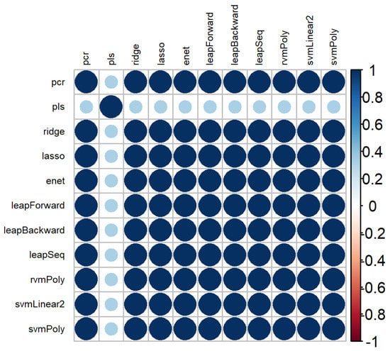
Figure 5.
Correlation plot of the variable rankings between the different machine learning methods used.
The ranking scores for the 100 most-relevant variables were represented in Figure 6. The vast majority of those variables came from the index database (IDB []) family. The 10 most relevant were:
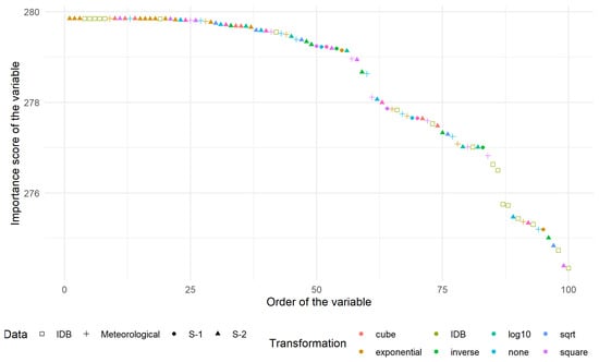
Figure 6.
Ranking score of the 100 most relevant variables distinguished according to the type of data (shape) and the transformation applied (colour).
- S2T.B06.10exp which corresponds to the exponential transformation of band 06 of S-2;
- S2T.B07.10exp which corresponds to the exponential transformation of band 07 of S-2;
- S2T.B08.10exp which corresponds to the exponential transformation of band 08f of S-2;
- IDB.032 known as Enhanced Vegetation Index;
- IDB.051 known as Hue;
- IDB.062 known as MCARI/MTVI2;
- IDB.071 known as mND680;
- IDB.221 known as Soil and Atmospherically Resistant Vegetation Index 2;
- CumT.DJ18.Last.10exp which corresponds to the exponential transformation of the degree-day with a basis of 18 C since the last CSH acquisition;
- S2T.B01.cube which corresponds to the cubic transformation of band 01 of S-2.
The number behind the point in the “IDB.XXX” represents the index in Henrich et al. []. Band 03, 04 and 05 of S-2 appeared in most indices. They corresponded respectively to green, red and near infra-red domains, which are known to be related to actual biomass (e.g., the NDVI ratio uses two of these bands). Another frequently appearing band was the first one, related to atmospheric correction and aerosol scattering. This suggested that there could be some residual effect of the pre-treatment concerning atmospheric condition.
The curve related to the multivariate linear models built from an increasing number of variables (previously ranked on the basis of their score) is shown in Figure 7 with the breakpoints highlighted with vertical lines. The dot-dashed breakpoints are the ones used in the analysis whilst the others (the plain lines) were left aside. The breakpoints taken into account in this study were related to linear models, including 7, 47, 111, 122 and 160 variables.
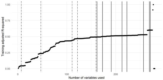
Figure 7.
Adjusted R-Squared curve trained on a cumulative number of variables sorted according to their ranking score. The breakpoints are represented with vertical lines. The dot-dashed lines correspond to the breakpoints taken into account, while the plain lines correspond to the other detected breakpoints.
3.3. Prediction of Compressed Sward Height (CSH)
From all subsets, approximately 50% of the 31 models run provided a RMSEcv lower than 100 mm of CSH (Table 5). Some models did not converge or provided extreme RMSEcv values. The models having RMSEcv values lower than 100 mm of CSH showed a tendency to decrease median RMSEcv values with an increase in the number of input variables. The minimum RMSEcv values were similar between subsets and lower than in the literature []. Figure 8 highlights the most powerful models based on their RMSEcv values. RF, cubist and enet models appeared to be highly repeatable between subsets. On the other hand, other models like the glm, lm, svmLinear2, leapSeq, ridge and svmPoly families showed a poor prediction ability.
Table 5.
Cross-validation performances of machine learning models run on the selected subsets.
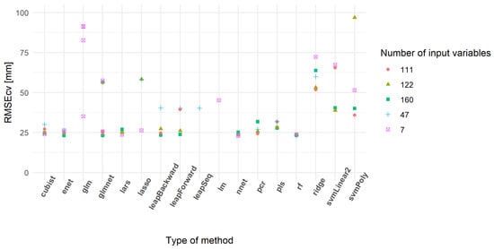
Figure 8.
Cross-validation root mean square error (RMSEcv) of the best-predicting models.
The prediction performances of the models were also assessed using an external validation dataset. As observed for the cross-validation (Table 5), some models did not provide realistic results (Table 6). The models with a validation RMSE lower than 100 mm showed a smaller range of variation than the one observed for the cross-validation. The minimum values of RMSE were also similar and confirm the potential interest of some developed models. Figure 9 shows the models having the lowest RMSEv. As observed in Figure 8, the rf, cubist and enet models seemed relevant as they had low RMSEv. Some models gained in terms of prediction capability, like rvmPoly that did not appear in Table 5 but well in Table 6. The distribution of RMSEv between subsets was relatively similar, except for the first subset. This could be related to a lack of information in the inputs of the model. In other words, some models using seven variables could be under-fitted.
Table 6.
Validation performances of models which converged during the cross-validation for all selected subsets.
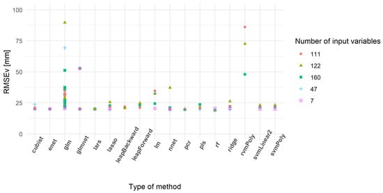
Figure 9.
Validation root mean square error (RMSEv) of the best models predicting compressed sward height (mm).
The best models should have low RMSEv and RMSEcv values, as well as a low difference between them. The lower the difference, the better the model’s robustness. Moreover, it is also important to have a distribution of the predicted values close to the one observed on the original dataset. Figure 10 developed the distribution of the actual CSH of the independent validation dataset and the CSH predicted by each model that provided realistic solutions on this dataset (i.e., NbOK model in Table 6). None of the models reproduced exactly the original distribution of the CSH. Two trends explained this differentiation: some models tended to group the prediction around the median of the distribution, and some models showed some saturation effect, resulting in a large amount of recording in the extreme classes. The cubist, nnet and rf methods and some linear regressions with variable selection were the methods that provided the best-fitting distribution curve. Some models provided extreme predictions.
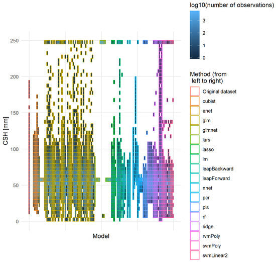
Figure 10.
Distribution of the original and predicted CSH values. All models that managed to provide a usable expression were used to predict CSH (mm) on the independent validation dataset. The y-axis was divided into parts of 5 mm and for each part the number of records were counted. To ease the representation, the number of observations was transformed into its logarithm of base 10.
The residuals were approximately centered on 0. Most models had a non-normal distribution of the residuals, given that their negative tail was often much larger than the positive one. The distribution of the residuals, according to the original CSH revealed that the most extreme residual values corresponded to CSH values near 50 mm of CSH for some glm models. Moreover, a higher absolute value of the residuals could be observed in the original CSH distribution extremes, meaning that all the information might not have been taken into account.
3.4. Effect of the Pixellation/Aggregation of Data
Beyond the pixel-base performances, the behavior of the models at the paddock scale was also assessed as the biomass that accounts for feed budgeting spread all over the parcel on which cattle graze. The RMSE of the training aggregated and of the validation aggregated dataset are summarised in Table 7. The lower threshold of around 19 mm of CSH that could be observed previously was completely blown up by the aggregation, with RMSE values reaching almost 4 mm of CSH in some cases. Unlike in the pixel analysis, the improvement of the quality indicators did not stand out for the validation dataset compared to the training one, although the RMSE was globally lower for the validation dataset. Two approaches were adopted in this table: on the one hand, the prediction was made solely on the parcel-scale aggregated data, and on the other hand, the prediction was made at the pixel level and then aggregated at the parcel-level. The first approach delivered better results for the calibration and the second for the independent validation dataset.
Table 7.
Summary of the RMSE [mm] of the models on the CSH data aggregated at the parcel level. The difference between “Training aggregated” and “Aggregated training” was that the first case corresponded to a prediction on the aggregated training dataset and the second to an aggregation of the prediction made on the training dataset at a pixel scale. The same goes for the validation items.
The RMSE decrease observed in Table 7 when the prediction was made on the pixel basis and then aggregated could be explained based on two different points of view. First, the variance of the reference datasets differed depending on the order of the prediction and aggregation. Secondly, a more materialistic explanation is the compensation of the sampling errors and the localization of the sampling: the GPS integrated to the RPM used did not have high precision, leading to positioning errors in the pixels. With the training data being comprised of medians of the records in each pixel, some records may have slipped from one pixel to another changing the value attributed to the pixel. The gathering of the information per parcel seemed to have erased a part of the error created. The effect of the difference in variance was taken into account by considering RPD.
A study of the prediction and the residuals similar to the one described above was performed on the validation dataset. The aggregation at the parcel-scale occurred after the prediction on the pixel. In general, the aggregation resulted in deleting the most extreme values and a linearisation of the distribution of the predictions. However, multiple behaviors could be distinguished. First, some models narrowed the scope of the response, others drifted this range, and finally, a few broadened the values explored. The distribution of the residuals tended to be centered on 0, although some models drifted completely like before. No obvious relationship appeared between the residuals and the predicted CSH except for the models that already showed a tendency to drift.
3.5. Best Performing Models
The models that performed the best, i.e., having a low RMSE of independent validation are shown in Table 8. It summarises the main statistical parameters of the 20 models having the lowest RMSE of independent validation on the pixellated dataset: the family, the number of input variables, the RMSEcv and RMSEv, and residual prediction deviation on the two possible aggregations (pre- and post-prediction) for both training and validation datasets. A svmLinear reached the highest RPD for the training phase, an enet model for the independent validation, and a cubist model stood out regarding all the aggregations together. Concerning the effect of aggregation, the RPD was globally higher for the models aggregated pre-prediction on the training dataset. This, as well as the high number of negative differences of RPD for the training dataset, suggested that the aggregation at the parcel-scale before prediction was the most relevant method. The RPD difference related to the validation dataset implied the opposite, which matches the results of Table 7.
Table 8.
Description of the main features of the best-performing models from the RMSE of validation on pixellated independent validation point of view.
The correlation values between the predictions of the models on the validation pixellated dataset are represented in Figure 11. As Figure 10 suggested, the predictions of the various models were not similar, as correlation values were low. However, some models showed high correlations within the same method like rf, nnet and pcr or out of the family, such as rf’s, nnet’s, glmnet, and cubist. Conversely, some models of the same family with quite similar RPD values in Table 8 had correlations close to zero.
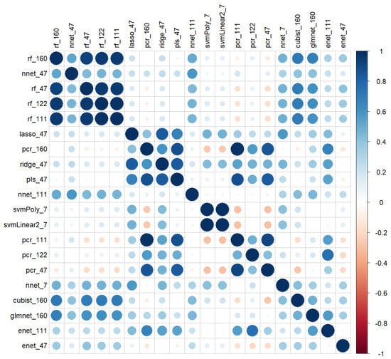
Figure 11.
Correlations of the predictions of the 20 best models on the basis of the RMSE of independent validation.
Other quality indicators were also studied for some of these models: for each method, only the model with the lowest RMSE was kept. Figure 12 represents the distribution of the original independent pixellated validation dataset and the prediction made on this dataset. It appeared that most models did shrink the range of values adopted, although some extreme values appeared. From this graph, the cubist and rf models were the models most capable of reproducing the original distribution of predicted values, closely followed by a glmnet based on a gaussian family and nnet models.
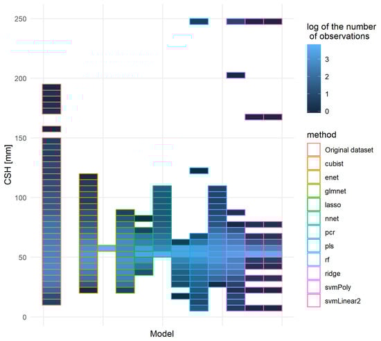
Figure 12.
Distribution of the original and predicted CSH values of the independent pixellated validation dataset for the 11 best models, one per method. Each set of predictions of the models occupied a spot on the x-axis and the original pixellated validation dataset was on the left. The order of the models was the following: cubist, enet, glmnet, lasso, nnet, pcr, pls, rf, ridge, svmPoly, svmLinear2. The vertical axis corresponds to the CSH distribution: the axis was divided into parts of 5mm of CSH and for each part the number of records was counted.
The erasure of the tails of the distribution of the predictions could be considered either as noise filtering or a loss of information. If this was a loss of information, it might complicate future detections of extreme cases. The subject noise filtering should be treated with caution. It could be interesting to recall that the parcels were divided into pixels of 10 m of resolution and the value associated with each pixel was the median of the values recorded in its range. A filtering step had thus already been applied. However, the amount of CSH recordings for each pixel was not constant. It implies that the filtering was not made equally. Some extreme values may have thus come through this filtering. Another factor in the noise filtering/erasure of the tails of the distribution of the prediction is the imbalance of the class used to train the model: the cross-validation occurred based on the date of acquisition, and no restriction had been set on the number of values in each sub-class of CSH which resulted in a training of the models that could have promoted central values. The application of some down-sampling techniques could be relevant to enlarge the scope of predictions.
Another point related to the distribution of the residuals was the trend to over- or under-estimate the actual value. The distribution of the residuals showed no clear trend: the center of gravity seemed to be positive, and the tail made of the negative values seemed to be more important than the one made of positive values of residuals. Table 9 summarises the percentage of positive and negative values for each model. The models tended to produce positive residuals, which meant that the predictions were globally higher than the actual value, except for the glmnet and cubist models. This indicated that there was a global over-estimation. However, this trend was not that pronounced for cubist and pls models.
Table 9.
Percentage of positive (%>0) and negative (%<0) residuals values for each model tested.
The analysis of the indicators of the quality of prediction and residuals at a pixel-scale with a 10 m resolution led to the selection of four best models for predicting CSH: the cubist model using 160 variables, the glmnet model of the gaussian family based on 160 variables, the rf model based on 160 variables and the nnet model based on 47 variables.
4. Discussion
The main objective of this work was to predict grass biomass in pastures on the basis of merged heterogeneous data sources of information, multiple variable transformations and a broad scope of ML methods.
The first adaptation was the use of CSH measurements instead of real grass biomass. The acceptance of this proxy (CSH) in the scientific community [,,,] and the ease of acquiring these data were two of the reasons that led to this choice. Although it could have been possible to convert the CSH records to biomass with an equation provided for similar sward species and meteorological conditions by the manufacturer of the rising platemeter, the conversion was not made in order to prevent any interference with cut height. The experimental farm had records of biomass and linked differences of CSH before and after cutting since 2015. Linear regressions were trained on this basis with multiple combinations of scenarios: the fixation or not of the intercept, the determination of the model for each parcel sampled or all of them, the use of dry or raw biomass (data not shown). Some seasonal trends stood out but no consistency in the coefficient could be observed within this dataset (the values of the regression coefficient ranged from 50 to 1500 for CSH expressed in millimeters), nor with the equations provided by the seller (the pool of linear regression coefficient for the dry biomass was distributed around 150). Cudlin et al. [] also faced a high variability in regression coefficient and intercept values. However, they had more observations of biomass and CSH combined—at least 24 for each regression compared to at best 10 records for each parcel for each period of the year in the case of the experimental farm. This means they could rely on their few significant relationships whilst the regression computed for the experimental farm was not resilient. Hakl et al. [] also had results showing varying reliability and significance. The combination of these studies showed the sensitivity of the conversion from CSH to biomass, probably due to the floristic composition and, together with Ferraro et al. [], their results underlined this sensibility to a seasonal effect whose expression might be more or less mitigated depending on the year and the location. Another aspect that could have been considered was the direct use of the biomass records mentioned before. However, they were acquired at a low frequency (approximately 49 days) and the bands mown to get this data were too small to occupy a full pixel scale. This means that the signal would have been noisy and blurred and the total amount of records would have been 239 since 2015, with some records acquired before the launch of S-2 satellites. The use of CSH measurements as the observed variable was also motivated by the ease of visualizing this data for farmers. Crémer [] uses another meaningful example in his advice to farmers: the height of the grass compared to the ankle position on a boot.
Nakagami (2016) and Cimbelli and Vitale (2017) had similar trends in the distribution of the heights: namely, a non-normal distribution with a lower threshold and a peak near the small values, although this was less pronounced in their data. This might be related to pasture management practices in Wallonia. To allow for optimal quality in the consumed herbage grazing management should aim to maintain a tight sward where perennial species dominate and have no time to flower and reproduce in a vegetative manner. Applying such management obviously has an impact on the lower representation of flower and seed heads of higher height in the database.
Multiple sources of information were integrated into this work. The faint grouping effect of variables seen in the representation of the variables on the two first principal components (Figure 4) confirmed the non-redundancy of the information brought by the different groups of variables studied and their transformations. Another aspect that proved the relevance of integrating all these variables is the appearance of each group of variables, with or without transformation, at the beginning of the ranking of variables (Figure 6). S-2 ranked first then meteorological data followed by S-1 from the 50th onwards. Although a seasonal effect was observed in the attempts at conversion from CSH to actual biomass, the time markers inserted within the dataset did not seem to bring that much information given that the first appearance is in the 131st place. The use of one unique dataset of meteorological data could have led to the under-training of the models concerning these variables. The implementation of a spatialized meteorological dataset is considered. The use of the first band of S-2 data and its rather higher position in the variable ranking indicate that there could be some kind of artifact/residual effect due to the pre-processing chain.
The sources of information mentioned above were integrated into their raw and transformed forms. The relevance of this integration was confirmed in the representation of the variables according to their decreasing ranking score (Figure 6). The “amplifying” transformations, i.e., cubic, exponential and square and the combinations of bands of S-2 data were the most represented at the beginning of the ranking, although the other transformations also appeared, albeit less often. This means that the data transformations highlighted parts of the information.
Multiple ML methods were trained on the dataset based on the hypothesis that some features used in the modeling could handle collinearity differently and detect different parts of information. The methods that could handle collinearity were used in the variable selection. It appeared that all of them, apart from the PLS, detected the same order of importance of the variables which was translated by the high Spearman correlation of the rankings. Although this high level of similarity could ensure the validity of the models, the dependence of the residuals on the original CSH slightly detected on the validation dataset indicated that all the information explaining CSH was not completely taken into account. The most promising models were a cubist, a glmnet of the gaussian family, a rf and a nnet models based on S-1, S-2 and meteorological data. While we could not find any article using glmnet in the literature, random forest, cubist and neural networks were related to spectral enhancement and prediction of other target variables, like leaf area index (LAI) [,,,,,,,,]. However, they were never used to predict biomass or CSH on pastures with S-1 and S-2 datasets.
The hypothesis of pixellation of CSH data made at the beginning of this work was possible thanks to the geolocation linked to the measurements on the pastures. The objective of this fractionation of the study area was to increase the number of records that could be used during the training of the ML models, while limiting noise due to the allocation of different CSH for the same set of combinations of satellite variables. To enable posterior comparisons, the metrics of quality were computed both at the pixel scale and the parcel scale for the models developed at the pixel scale. This revealed that with and without aggregation, and whatever the aggregation method, the best-fitted models achieved better performances than the 29 mm RMSE shown by Cimbelli and Vitale []. They were the only ones to provide similar metrics in a similar context, although their height corresponded to the mean height computed on a picture instead of a CSH. The pixellation and aggregation processes acted as a partial filter concerning extreme values: the pixellation led to the erasure of the most extreme values for some pixels with the median filter, and the aggregation did the same with a mean filter.
One way to increase the size of the dataset could have been to create a continuum of CSH values within the parcels by using a kriging-like technique. However, this would mean that each record of CSH used would not have been completely independent from the others, given that a huge part of them would have been created as a combination of other measurements. Other types of gap-filling techniques were omitted due to their inherent complexity: sets of records on cloudy days were discarded because they made the use of S-2 data meaningless. A way to avoid this decrease in the dataset size would have been to use tiles acquired on the nearest dates and interpolate the values for each pixel. However, this would have required that the pastures would have witnessed no change in their management or condition: no removal nor addition of cows, nor any other operation like fertilization or mowing. Another obstacle to this process is the long-term archiving policy of ESA which complexified the acquisition of all relevant tiles, especially for the oldest ones. A similar problem of continuity in practices was dealt with using an approximation: the CSH data were not acquired exactly at the same time as S-1 and S-2 data. In this case, the closest tile in time was used, assuming that the frequency of satellite data acquisition is high enough to avoid major changes in pasture condition.
The future application of the models will be their integration within a DSS for the use of Walloon farmers. The objective will be to provide the farmers with information regarding the quantity of feed available on pastures. This means that the aggregated value of the predictions at the pixel-scale will probably be used. Filtering of extreme values would reveal useful for this assessment but the information about the refusals will be lost. The global over- and underestimation trend shown in Table 9 should be inserted in the DSS and treated with caution: an imprecision inherent to the sampling method using the rising platemeter has to be kept in mind. That is, it measures heights with a count of clicks on a ratchet and then converts this to CSH. The conversion is a source of error, and McSweeney et al. [] warn that this type of platemeter often under-estimates actual CSH height. Another source of the unreliability of the developed models is the lack of diversity in the farms that were used and more importantlyin the diversity of pasture botanical composition, soil types, fertility and management practices. The use of a completely independent validation dataset offsets this bias and imitated the future behavior of the models on other farms.
5. Conclusions
The main objective of this work was to test the following hypothesis: the use of various sources of information and multiple transformations of these data as inputs for a broad range of machine learning methods may improve predictions of CSH in pastures. The combination of sources of information, data transformations, and multiple machine learning methods allowed the development of more precise models than previously described in the literature. Four models stood out: a cubist, a glmnet, a neural network and a random forest-based model. They were all based on Sentinel-1 sigma nought, Sentinel-2 reflectance and meteorological data. Their RMSE of independent validation was around 19 mm of CSH at the pixel-level. To better train the models, more records will be gathered in the years to come, in Wallonia and possibly internationally. The models trained through this framework will be used to establish a tool to help farmers in their daily decision making. It is also planned to enable prediction at a larger scale, include an extreme case detection in the predictions and sampling the places where the extreme cases did occur to increase the resilience of the models. Moreover, for both the DSS and large scale prediction, a combination of the outputs is considered, given that the similarity of distribution does not reflect the different repartitions of the predictions.
Author Contributions
Conceptualization, C.N. and H.S.; software, C.N., A.T. and B.T.; validation, A.T., I.D., F.L., B.T., Y.C., J.B. and H.S.; formal analysis, C.N., A.T. and H.S.; resources, I.D. and F.L.; data curation, C.N., A.T., I.D., F.L., B.T., Y.C., J.B. and H.S.; writing—original draft preparation, C.N.; writing—review and editing, A.T., I.D., F.L., B.T., Y.C., J.B. and H.S.; visualization, C.N. and H.S.; supervision, H.S.; project administration, H.S. All authors have read and agreed to the published version of the manuscript.
Funding
This research received no external funding.
Institutional Review Board Statement
Not applicable.
Informed Consent Statement
Not applicable.
Data Availability Statement
The data presented in this study are available on request from the corresponding author. The data are not publicly available due to privacy issues.
Acknowledgments
The authors would like to thank the ‘Wallonie agrigulture SPW’ for funding the ROAD-STEP project and this study. This work contains modified Copernicus Sentinel data (2020).
Conflicts of Interest
The authors declare no conflict of interest.
Abbreviations
The following abbreviations are used in this manuscript:
| CSH | Compressed sward height |
| DSS | Decision support system |
| PGSUS | Pasture Growth Simulation Using Smalltalk |
| MostGG | Moorepark St Gilles grass growth model |
| SAR | synthetic-aperture radar |
| C-SAR | synthetic-aperture radar in the C band data |
| CRS | Coordinate reference system |
References
- Hennessy, D.; Delaby, L.; van den Pol-van Dasselaar, A.; Shalloo, L. Increasing Grazing in Dairy Cow Milk Production Systems in Europe. Sustainability 2020, 12, 2443. [Google Scholar] [CrossRef]
- Elgersma, A. Grazing increases the unsaturated fatty acid concentration of milk from grass-fed cows: A review of the contributing factors, challenges and future perspectives. Eur. J. Lipid Sci. Technol. 2015, 117, 1345–1369. [Google Scholar] [CrossRef]
- Lessire, F.; Jacquet, S.; Veselko, D.; Piraux, E.; Dufrasne, I. Evolution of grazing practices in Belgian dairy farms: Results of two surveys. Sustainability 2019, 11, 3997. [Google Scholar] [CrossRef]
- Cros, M.J.; Garcia, F.; Martin-Clouaire, R. SEPATOU: A Decision Support System for the Management of Rotational Grazing in a Dairy Production. In Proceedings of the 2nd European Conference on Information Technology in Agriculture, Bonn, Germany, 27–30 September 1999; pp. 549–557. [Google Scholar]
- Amalero, E.G.; Ingua, G.L.; Erta, G.B.; Emanceau, P.L. A biophysical dairy farm model to evaluate rotational grazing management strategies. Agronomie 2003, 23, 407–418. [Google Scholar] [CrossRef]
- Romera, A.J.; Beukes, P.; Clark, C.; Clark, D.; Levy, H.; Tait, A. Use of a pasture growth model to estimate herbage mass at a paddock scale and assist management on dairy farms. Comput. Electron. Agric. 2010, 74, 66–72. [Google Scholar] [CrossRef]
- Romera, A.; Beukes, P.; Clark, D.; Clark, C.; Tait, A. Pasture growth model to assist management on dairy farms: Testing the concept with farmers. Grassl. Sci. 2013, 59, 20–29. [Google Scholar] [CrossRef]
- Ruelle, E.; Hennessy, D.; Delaby, L. Development of the Moorepark St Gilles grass growth model (MoSt GG model): A predictive model for grass growth for pasture based systems. Eur. J. Agron. 2018, 99, 80–91. [Google Scholar] [CrossRef]
- Moeckel, T.; Safari, H.; Reddersen, B.; Fricke, T.; Wachendorf, M. Fusion of ultrasonic and spectral sensor data for improving the estimation of biomass in grasslands with heterogeneous sward structure. Remote Sens. 2017, 9, 98. [Google Scholar] [CrossRef]
- Cudlín, O.; Hakl, J.; Hejcman, M.; Cudlín, P. The use of compressed height to estimate the yield of a differently fertilized meadow. Plant Soil Environ. 2018, 64, 76–81. [Google Scholar] [CrossRef]
- Lussem, U.; Bolten, A.; Menne, J.; Gnyp, M.L.; Schellberg, J.; Bareth, G. Estimating biomass in temperate grassland with high resolution canopy surface models from UAV-based RGB images and vegetation indices. J. Appl. Remote Sens. 2019, 13, 034525. [Google Scholar] [CrossRef]
- Laca, E.A.; Demment, M.W.; Winckel, J.; Kie, J.G. Comparison of weight estimate and rising-plate meter methods to measure herbage mass of a mountain meadow. J. Range Manag. 1989, 42, 71–75. [Google Scholar] [CrossRef]
- French, P.; O’Brien, B.; Shalloo, L. Development and adoption of new technologies to increase the efficiency and sustainability of pasture-based systems. Anim. Prod. Sci. 2015, 55, 931–935. [Google Scholar] [CrossRef]
- MacAdam, J.; Hunt, S. Using a Rising Plate Meter to Determine Paddock Size for Rotational Grazing; Utah State University Extension Bulletin: Logan, UT, USA, 2015. [Google Scholar]
- Gargiulo, J.; Clark, C.; Lyons, N.; de Veyrac, G.; Beale, P.; Garcia, S. Spatial and temporal pasture biomass estimation integrating electronic plate meter, planet cubesats and sentinel-2 satellite data. Remote Sens. 2020, 12, 3222. [Google Scholar] [CrossRef]
- Wang, J.; Xiao, X.; Bajgain, R.; Starks, P.; Steiner, J.; Doughty, R.B.; Chang, Q. Estimating leaf area index and aboveground biomass of grazing pastures using Sentinel-1, Sentinel-2 and Landsat images. ISPRS J. Photogramm. Remote Sens. 2019, 154, 189–201. [Google Scholar] [CrossRef]
- Hakl, J.; Hrevušová, Z.; Hejcman, M.; Fuksa, P. The use of a rising plate meter to evaluate lucerne (Medicago sativa L.) height as an important agronomic trait enabling yield estimation. Grass Forage Sci. 2012, 67, 589–596. [Google Scholar] [CrossRef]
- Crémer, S. La Gestion des Prairies—Notes de Cours 2015–2016; Fourrages-mieux, Marche-en-Famenne: Marloie, Belgium, 2015; pp. 1–142. [Google Scholar]
- Nakagami, K. A method for approximate on-farm estimation of herbage mass by using two assessments per pasture. Grass Forage Sci. 2016, 71, 490–496. [Google Scholar] [CrossRef]
- Fricke, T.; Wachendorf, M. Combining ultrasonic sward height and spectral signatures to assess the biomass of legume-grass swards. Comput. Electron. Agric. 2013, 99, 236–247. [Google Scholar] [CrossRef]
- Bareth, G.; Schellberg, J. Replacing Manual Rising Plate Meter Measurements with Low-cost UAV-Derived Sward Height Data in Grasslands for Spatial Monitoring. PFG J. Photogramm. Remote. Sens. Geoinf. Sci. 2018, 86, 157–168. [Google Scholar] [CrossRef]
- Legg, M.; Bradley, S. Ultrasonic Arrays for Remote Sensing of Pasture Biomass. Remote Sens. 2019, 12, 111. [Google Scholar] [CrossRef]
- Rayburn, E.B.; Lozier, J.D.; Sanderson, M.A.; Smith, B.D.; Shockey, W.L.; Seymore, D.A.; Fultz, S.W. Alternative Methods of Estimating Forage Height and Sward Capacitance in Pastures Can Be Cross Calibrated. Forage Grazinglands 2007, 5, 1–6. [Google Scholar] [CrossRef]
- Lopez diaz, J.; Gonzalez-rodriguez, A. Measuring grass yield by non-destructive methods. J. Chem. Inf. Model. 2013, 53, 1689–1699. [Google Scholar] [CrossRef]
- Cimbelli, A.; Vitale, V. Grassland height assessment by satellite images. Adv. Remote Sens. 2017, 6, 40–53. [Google Scholar] [CrossRef]
- Ancin-Murguzur, F.J.; Taff, G.; Davids, C.; Tømmervik, H.; Mølmann, J.; Jørgensen, M. Yield estimates by a two-step approach using hyperspectral methods in grasslands at high latitudes. Remote Sens. 2019, 11, 400. [Google Scholar] [CrossRef]
- Zeng, L.; Chen, C. Using remote sensing to estimate forage biomass and nutrient contents at different growth stages. Biomass Bioenergy 2018, 115, 74–81. [Google Scholar] [CrossRef]
- Tiscornia, G.; Baethgen, W.; Ruggia, A.; Do Carmo, M.; Ceccato, P. Can we Monitor Height of Native Grasslands in Uruguay with Earth Observation? Remote Sens. 2019, 11, 1801. [Google Scholar] [CrossRef]
- Michez, A.; Philippe, L.; David, K.; Sébastien, C.; Christian, D.; Bindelle, J. Can low-cost unmanned aerial systems describe the forage quality heterogeneity? Insight from a timothy pasture case study in southern Belgium. Remote Sens. 2020, 12, 1650. [Google Scholar] [CrossRef]
- Borra-Serrano, I.; De Swaef, T.; Muylle, H.; Nuyttens, D.; Vangeyte, J.; Mertens, K.; Saeys, W.; Somers, B.; Roldán-Ruiz, I.; Lootens, P. Canopy height measurements and non-destructive biomass estimation of Lolium perenne swards using UAV imagery. Grass Forage Sci. 2019, 74, 356–369. [Google Scholar] [CrossRef]
- Michez, A.; Lejeune, P.; Bauwens, S.; Lalaina Herinaina, A.A.; Blaise, Y.; Muñoz, E.C.; Lebeau, F.; Bindelle, J. Mapping and monitoring of biomass and grazing in pasture with an unmanned aerial system. Remote Sens. 2019, 11, 473. [Google Scholar] [CrossRef]
- Shalloo, L.; Donovan, M.O.; Leso, L.; Werner, J.; Ruelle, E.; Geoghegan, A.; Delaby, L.; Leary, N.O. Review: Grass-based dairy systems, data and precision technologies. Animal 2018, 12, S262–S271. [Google Scholar] [CrossRef]
- Eastwood, C.R.; Dela Rue, B.T.; Gray, D.I. Using a ‘network of practice’ approach to match grazing decision-support system design with farmer practice. Anim. Prod. Sci. 2017, 57, 1536–1542. [Google Scholar] [CrossRef]
- McSweeney, D.; Coughlan, N.E.; Cuthbert, R.N.; Halton, P.; Ivanov, S. Micro-sonic sensor technology enables enhanced grass height measurement by a Rising Plate Meter. Inf. Process. Agric. 2019, 6, 279–284. [Google Scholar] [CrossRef]
- Jouven, M.; Carrère, P.; Baumont, R. Model predicting dynamics of biomass, structure and digestibility of herbage in managed permanent pastures. 1. Model description. Grass Forage Sci. 2006, 61, 112–124. [Google Scholar] [CrossRef]
- Thornley, J.H.M. Grassland Dynamics: An Ecosystem Simulation Model; CAB International: Wallingford, UK, 1998. [Google Scholar]
- Sándor, R.; Ehrhardt, F.; Brilli, L.; Carozzi, M.; Recous, S.; Smith, P.; Snow, V.; Soussana, J.F.; Dorich, C.D.; Fuchs, K.; et al. The use of biogeochemical models to evaluate mitigation of greenhouse gas emissions from managed grasslands. Sci. Total Environ. 2018, 642, 292–306. [Google Scholar] [CrossRef] [PubMed]
- Brisson, N.; Mary, B.; Ripoche, D.; Jeuffroy, M.H.; Ruget, F.; Nicoullaud, B.; Gate, P.; Devienne-Barret, F.; Antonioletti, R.; Durr, C.; et al. STICS: A generic model for the simulation of crops and their water and nitrogen balances. I. Theory and parameterization applied to wheat and corn. Agronomie 1998, 18, 311–346. [Google Scholar] [CrossRef]
- McDonnell, J.; Brophy, C.; Ruelle, E.; Shalloo, L.; Lambkin, K.; Hennessy, D. Weather forecasts to enhance an Irish grass growth model. Eur. J. Agron. 2019, 105, 168–175. [Google Scholar] [CrossRef]
- Tamm, T.; Zalite, K.; Voormansik, K.; Talgre, L. Relating Sentinel-1 interferometric coherence to mowing events on grasslands. Remote Sens. 2016, 8, 802. [Google Scholar] [CrossRef]
- Stendardi, L.; Karlsen, S.R.; Niedrist, G.; Gerdol, R.; Zebisch, M.; Rossi, M.; Notarnicola, C. Exploiting time series of Sentinel-1 and Sentinel-2 imagery to detect meadow phenology in mountain regions. Remote Sens. 2019, 11, 542. [Google Scholar] [CrossRef]
- Shoko, C.; Mutanga, O.; Dube, T. Determining optimal new generation satellite derived metrics for accurate C3 and C4 grass species aboveground biomass estimation in South Africa. Remote Sens. 2018, 10, 564. [Google Scholar] [CrossRef]
- Kumar, L.; Sinha, P.; Taylor, S.; Alqurashi, A.F. Review of the use of remote sensing for biomass estimation to support renewable energy generation. J. Appl. Remote Sens. 2015, 9, 097696. [Google Scholar] [CrossRef]
- Punalekar, S.M.; Verhoef, A.; Quaife, T.L.; Humphries, D.; Bermingham, L.; Reynolds, C.K. Application of Sentinel-2A data for pasture biomass monitoring using a physically based radiative transfer model. Remote Sens. Environ. 2018, 218, 207–220. [Google Scholar] [CrossRef]
- Mutanga, O.; Shoko, C. Monitoring the spatio-temporal variations of C3/C4 grass species using multispectral satellite data. IGARSS 2018, 2018, 8988–8991. [Google Scholar] [CrossRef]
- Darvishzadeh, R.; Wang, T.; Skidmore, A.; Vrieling, A.; O’Connor, B.; Gara, T.W.; Ens, B.J.; Paganini, M. Analysis of Sentinel-2 and rapidEye for retrieval of leaf area index in a saltmarsh using a radiative transfer model. Remote Sens. 2019, 11, 671. [Google Scholar] [CrossRef]
- Garioud, A.; Giordano, S.; Valero, S.; Mallet, C. Challenges in Grassland Mowing Event Detection with Multimodal Sentinel Images. MultiTemp 2019, 1–4. [Google Scholar] [CrossRef]
- Alves, R.; Näsi, R.; Niemeläinen, O.; Nyholm, L.; Alhonoja, K.; Kaivosoja, J.; Jauhiainen, L.; Viljanen, N.; Nezami, S.; Markelin, L. Remote Sensing of Environment Machine learning estimators for the quantity and quality of grass swards used for silage production using drone-based imaging spectrometry and photogrammetry. Remote Sens. Environ. 2020, 246, 111830. [Google Scholar] [CrossRef]
- Fernández-Delgado, M.; Sirsat, M.S.; Cernadas, E.; Alawadi, S.; Barro, S.; Febrero-Bande, M. An extensive experimental survey of regression methods. Neural Netw. 2019, 111, 11–34. [Google Scholar] [CrossRef]
- García, R.; Aguilar, J.; Toro, M.; Pinto, A.; Rodríguez, P. A systematic literature review on the use of machine learning in precision livestock farming. Comput. Electron. Agric. 2020, 179, 105826. [Google Scholar] [CrossRef]
- R Core Team. R: A Language and Environment for Statistical Computing; R Foundation for Statistical Computing: Vienna, Austria, 2019. [Google Scholar]
- RStudio Team. RStudio: Integrated Development Environment for R; RStudio, Inc.: Boston, MA, USA, 2019. [Google Scholar]
- Moot, D.J.; Scott, W.R.; Roy, A.M.; Nicholls, A.C.; Scott, W.R.; Roy, A.M.; Base, A.C.N. Base temperature and thermal time requirements for germination and emergence of temperate pasture species. N. Z. J. Agric. Res. 2010, 8233, 15–25. [Google Scholar] [CrossRef]
- Balocchi, O.; Alonso, M.; Keim, J.P. Water-Soluble Carbohydrate Recovery in Pastures of Perennial Ryegrass (Lolium perenne L.) and Pasture Brome (Bromus valdivianus Phil.) Under Two Defoliation Frequencies Determined by Thermal Time. Agriculture 2020, 10, 563. [Google Scholar] [CrossRef]
- Anandhi, A. Growing Degree Days—Ecosystem Indicator for changing diurnal temperatures and their impact on corn growth stages in Kansas. Ecol. Indic. 2016, 61, 149–158. [Google Scholar] [CrossRef]
- Salvucci, M.E.; Osteryoung, K.W.; Crafts-brandner, S.J.; Vierling, E. Exceptional Sensitivity of Rubisco Activase to Thermal Denaturation in Vitro and in Vivo 1. Plant Physiol. 2001, 127, 1053–1064. [Google Scholar] [CrossRef]
- Greco, M.; Parry, A.J.; Andralojc, J.; Carmo-silva, A.E.; Alonso, H. Rubisco activity and regulation targets for crop in DNA In Posidonia oceanica cadmium as induces changes improvement methylation and chromatin patterning. J. Exp. Bot. 2013, 64, 717–730. [Google Scholar] [CrossRef]
- Copernicus. Open Access Hub. 2018. Available online: https://scihub.copernicus.eu/ (accessed on 7 December 2020).
- European Space Agency. Sen2Cor | STEP; European Space Agency: Paris, France, 2018. [Google Scholar]
- Schwalb-Willmann, J. getSpatialData: Get Different Kinds of Freely Available Spatial Datasets. R Package Version 0.0.4. 2018. Available online: https://rdrr.io/github/16EAGLE/getSpatialData/f/NEWS.md (accessed on 7 December 2020).
- Filipponi, F. Sentinel-1 GRD Preprocessing Workflow. Proceedings 2019, 18, 11. [Google Scholar] [CrossRef]
- Filipponi, F. Sentinel-1_GRD_Preprocessing_ Standard Workflow for the Preprocessing of Sentinel-1 GRD Satellite Data; MDPI: Basel, Switzerland, 2020. [Google Scholar]
- ESA. SNAP—ESA Sentinel Application Platform v7.0.0; ESA: Paris, France, 2020. [Google Scholar]
- Rudant, J.P.; Frison, P.L. Télédéction radar: De l’image d’intensité initiale au choix du mode de calibation des coefficients de diffusion beta nought, sigma nought et gamma nought. Revue Française de Photogrammétrie et Télédétection 2019, 219–220, 19–28. [Google Scholar]
- Ranghetti, L.; Busetto, L. Sen2r: Find, Download and Process Sentinel-2 Data. R Package Version 1.2.1. 2019. Available online: https://doi.org/10.5281/zenodo.1240384 (accessed on 7 December 2020).
- Mueller-Wilm, U. Sen2Cor Configuration and User Manual; ESA: Paris, France, 2016. [Google Scholar]
- GDAL/OGR Contributors. GDAL/OGR Geospatial Data Abstraction Software Library. Open Source Geospatial Foundation. 2020. Available online: https://gdal.org/ (accessed on 7 December 2020).
- Higgins, S.; Schellberg, J.; Bailey, J.S. Improving productivity and increasing the efficiency of soil nutrient management on grassland farms in the UK and Ireland using precision agriculture technology. Eur. J. Agron. 2019, 106, 67–74. [Google Scholar] [CrossRef]
- Lugassi, R.; Zaady, E.; Goldshleger, N.; Shoshany, M.; Chudnovsky, A. Spatial and temporal monitoring of pasture ecological quality: Sentinel-2-based estimation of crude protein and neutral detergent fiber contents. Remote Sens. 2019, 11, 799. [Google Scholar] [CrossRef]
- Ruelle, E.; Delaby, L. Pertinence du Modèle Moorepark-St Gilles Grass Growth dans les conditions climatiques de l Ouest de la France; Description du modèle Moorepark-St Gilles Grass Growth a) b). 2017, pp. 158–159. Available online: https://hal.archives-ouvertes.fr/hal-01595315/ (accessed on 7 December 2020).
- Dowle, M.; Srinivasan, A. data.table: Extension of ‘data.frame’. R Package Version 1.12.8. 2019. Available online: https://cran.r-project.org/web/packages/data.table/index.html (accessed on 7 December 2020).
- Wickham, H.; François, R.; Henry, L.; Müller, K. dplyr: A Grammar of Data Manipulation; R Package Version 0.8.3. 2019. Available online: https://dplyr.tidyverse.org/ (accessed on 7 December 2020).
- Pebesma, E. Simple Features for R: Standardized Support for Spatial Vector Data. R J. 2018, 10, 439–446. [Google Scholar] [CrossRef]
- Pebesma, E.J.; Bivand, R.S. Classes and methods for spatial data in R. R News 2005, 5, 9–13. [Google Scholar]
- Bivand, R.S.; Pebesma, E.; Gomez-Rubio, V. Applied Spatial Data Analysis with R, 2nd ed.; Springer: New York, NY, USA, 2013. [Google Scholar]
- Hijmans, R.J. Raster: Geographic Data Analysis and Modeling. R Package Version 3.0-7. 2019. Available online: https://rdrr.io/cran/raster/ (accessed on 7 December 2020).
- Bengtsson, H. Future: Unified Parallel and Distributed Processing in R for Everyone. R Package Version 1.16.0. 2020. Available online: https://cran.r-project.org/web/packages/future/index.html (accessed on 7 December 2020).
- Bengtsson, H. Future.Apply: Apply Function to Elements in Parallel using Futures; R Package Version 1.4.0. 2020. Available online: https://cran.r-project.org/web/packages/future.apply/index.html (accessed on 7 December 2020).
- Ali, I.; Cawkwell, F.; Dwyer, E.; Barrett, B.; Green, S. Satellite remote sensing of grasslands: From observation to management. J. Plant Ecol. 2016, 9, 649–671. [Google Scholar] [CrossRef]
- Henrich, V.; Götze, C.; Jung, A.; Sandow, C.; Thürkow, D.; Cornelia, G. Development of an online indices database: Motivation, concept and implementation. In Proceedings of the 6th EARSeL Imaging Spectroscopy SIG Workshop Innovative Tool for Scientific and Commercial Environment Applications, Tel Aviv, Israel, 16–18 March 2009. [Google Scholar]
- IDB—Sensor_ Sentinel-2A. Available online: https://www.indexdatabase.de/db/s-single.php?id=96 (accessed on 23 January 2021).
- Lê, S.; Josse, J.; Husson, F. FactoMineR: A Package for Multivariate Analysis. J. Stat. Softw. 2008, 25, 1–18. [Google Scholar] [CrossRef]
- Kuhn, M. Caret: Classification and Regression Training. R Package Version 6.0-85. 2020. Available online: http://topepo.github.io/caret/index.html (accessed on 23 January 2021).
- Ali, I.; Greifeneder, F.; Stamenkovic, J.; Neumann, M.; Notarnicola, C. Review of machine learning approaches for biomass and soil moisture retrievals from remote sensing data. Remote Sens. 2015, 7, 16398–16421. [Google Scholar] [CrossRef]
- Houborg, R.; McCabe, M.F. A hybrid training approach for leaf area index estimation via Cubist and random forests machine-learning. ISPRS J. Photogramm. Remote Sens. 2018, 135, 173–188. [Google Scholar] [CrossRef]
- Houborg, R.; McCabe, M.F. High-Resolution NDVI from planet’s constellation of earth observing nano-satellites: A new data source for precision agriculture. Remote Sens. 2016, 8, 768. [Google Scholar] [CrossRef]
- Houborg, R.; McCabe, M.F. A Cubesat enabled Spatio-Temporal Enhancement Method (CESTEM) utilizing Planet, Landsat and MODIS data. Remote Sens. Environ. 2018, 209, 211–226. [Google Scholar] [CrossRef]
- Ali, I.; Cawkwell, F.; Green, S.; Dwyer, N. Application of statistical and machine learning models for grassland yield estimation based on a hypertemporal satellite remote sensing time series. In Proceedings of the IEEE Geoscience and Remote Sensing Symposium, Quebec City, QC, Canada, 13–18 July 2014; pp. 5060–5063. [Google Scholar] [CrossRef]
- Ali, I.; Cawkwell, F.; Dwyer, E.; Green, S. Modeling Managed Grassland Biomass Estimation by Using Multitemporal Remote Sensing Data-A Machine Learning Approach. IEEE J. Sel. Top. Appl. Earth Obs. Remote Sens. 2017, 10, 3254–3264. [Google Scholar] [CrossRef]
- Taravat, A.; Wagner, M.; Oppelt, N. Automatic Grassland Cutting Status Detection in the Context of Spatiotemporal Sentinel-1 Imagery Analysis and Artificial Neural Networks. Remote Sens. 2019, 11, 711. [Google Scholar] [CrossRef]
- Shi, Y.; Xiong, F.; Xiu, R.; Liu, Y. A comparative study of relevant vector machine and support vector machine in uncertainty analysis. In Proceedings of the 2013 International Conference on Quality, Reliability, Risk, Maintenance, and Safety Engineering (QR2MSE), Chengdu, China, 15–18 July 2013; pp. 469–472. [Google Scholar] [CrossRef]
- Hanrahan, L.; Geoghegan, A.; O’Donovan, M.; Griffith, V.; Ruelle, E.; Wallace, M.; Shalloo, L. PastureBase Ireland: A grassland decision support system and national database. Comput. Electron. Agric. 2017, 136, 193–201. [Google Scholar] [CrossRef]
- Murphy, D.J.; O’ Brien, B.; Askari, M.S.; McCarthy, T.; Magee, A.; Burke, R.; Murphy, M.D. GrassQ—A holistic precision grass measurement and analysis system to optimize pasture based livestock production. In Proceedings of the 2019 ASABE Annual International Meeting, Boston, MA, USA, 7–10 July 2019. [Google Scholar] [CrossRef][Green Version]
- Ferraro, F.P.; Nave, R.L.; Sulc, R.M.; Barker, D.J. Seasonal variation in the rising plate meter calibration for forage mass. Agron. J. 2012, 104, 1–6. [Google Scholar] [CrossRef]
- Houborg, R.; McCabe, M.F. Daily retrieval of NDVI and LAI at 3 m resolution via the fusion of CubeSat, Landsat, and MODIS data. Remote Sens. 2018, 10, 890. [Google Scholar] [CrossRef]
Publisher’s Note: MDPI stays neutral with regard to jurisdictional claims in published maps and institutional affiliations. |
© 2021 by the authors. Licensee MDPI, Basel, Switzerland. This article is an open access article distributed under the terms and conditions of the Creative Commons Attribution (CC BY) license (http://creativecommons.org/licenses/by/4.0/).