Abstract
In this study, we examined the natural recovery of mangroves in abandoned shrimp ponds located in the Wunbaik Mangrove Forest (WMF) in Myanmar using artificial neural network (ANN) classification and a change detection approach with Sentinel-2 satellite images. In 2020, we conducted various experiments related to mangrove classification by tuning input features and hyper-parameters. The selected ANN model was used with a transfer learning approach to predict the mangrove distribution in 2015. Changes were detected using classification results from 2015 and 2020. Naturally recovering mangroves were identified by extracting the change detection results of three abandoned shrimp ponds selected during field investigation. The proposed method yielded an overall accuracy of 95.98%, a kappa coefficient of 0.92, mangrove and non-mangrove precisions of 0.95 and 0.98, respectively, recalls of 0.96, and F1 scores of 0.96 for the 2020 classification. For the 2015 prediction, transfer learning improved model performance, resulting in an overall accuracy of 97.20%, a kappa coefficient of 0.94, mangrove and non-mangrove precisions of 0.98 and 0.96, respectively, recalls of 0.98 and 0.97, and F1 scores of 0.96. The change detection results showed that mangrove forests in the WMF slightly decreased between 2015 and 2020. Naturally recovering mangroves were detected at approximately 50% of each abandoned site within a short abandonment period. This study demonstrates that the ANN method using Sentinel-2 imagery and topographic and canopy height data can produce reliable results for mangrove classification. The natural recovery of mangroves presents a valuable opportunity for mangrove rehabilitation at human-disturbed sites in the WMF.
1. Introduction
Mangrove forests provide highly valuable ecosystem services consisting of tangible goods, such as wood and non-wood products, and intangible services, such as the protection of coastal regions from storms and wave attacks and the sequestration of substantial volumes of carbon dioxide [1,2]. Despite these invaluable services, mangrove forests worldwide are being depleted at an alarming rate every year because of anthropogenic pressures, such as the development of aquaculture, agricultural expansion, oil plantations, and urbanization [3,4,5]. Mangroves possess a high capacity for self-recovery; this facilitates mangrove rehabilitation. Mangrove self-recovery involves the natural restoration of mangrove species in a deforested area if environmental parameters, such as natural hydrology, salinity, and site elevation, satisfy the preferences of seeds or propagules dispersed with tidal flow [6,7]. However, limited research has been conducted to address the natural recovery of mangroves in rehabilitation programs. This study highlights the natural recovery of mangroves after human disturbance using remote sensing classification and a change detection approach.
The Wunbaik Mangrove Forest (WMF) in Myanmar is one of the largest remaining mangrove forests in the world and provides ecological, environmental, and socio-economic goods and services to the local community. Due to the expansion of aquaculture and agriculture, WMF has experienced severe degradation since the 1990s. According to the 2011 Food and Agricultural Organization (FAO) inventory [8], WMF possesses abundant seed productivity and a high mangrove species germination rate and is suitable for examining the natural recovery of mangroves depleted by human disturbances. Despite the presence of such a large remnant mangrove forest with a diverse range of species, there has been a prominent information gap regarding mangrove distribution and changes since 2014. Current and accurate information is necessary before implementing any restoration efforts for sustainable mangrove management.
Mangroves are under threat from natural and anthropogenic disturbances; however, accessing reliable and accurate information for many mangrove forests worldwide is difficult [9]. Remote sensing classification contributes to the provision of reliable information for different research topics, such as mangrove extent mapping, species identification, and estimation of above-ground biomass, contributing to the sustainable management of mangrove forests [10,11]. However, classification accuracy is highly variable depending on the performance of the selected classifier because each classification method has benefits and drawbacks [12]. Machine learning is an emerging advanced classification methodology in which supervised classifiers, such as maximum likelihood, random forest (RF), support vector machine (SVM), and artificial neural networks (ANNs), can outperform traditional unsupervised classification [13]. In mangrove remote sensing, many studies have reported that supervised classification is superior to unsupervised approaches [14,15,16]. Supervised machine learning classifiers, such as RF, SVM, classification and regression tree, and regularization in two discriminant analysis (RDA), have been compared and evaluated for mangrove cover changes [17,18,19]. However, ANNs require extensive training data and are rarely applied in mangrove classification. However, they have been widely used in many fields of remote sensing classification because of promising results and model robustness [20,21,22,23].
In terms of the role of remotely sensed data, the effect of input features is a key component in image classification. Many mangrove studies have been conducted using optical images with different resolutions (e.g., IKONOS, QuickBird, WorldView-3, Landsat series, and SPOT), synthetic aperture radar (SAR) data, and airborne hyperspectral data [11,24,25,26,27,28]. The launch of the Sentinel-2 satellite by the European Space Agency in 2015 provided a valuable opportunity for the remote sensing community to develop classification approaches in a wide variety of fields [29]. Owing to the advantage of spectral, temporal, and spatial resolutions of freely accessible multi-spectral bands, Sentinel-2 imagery outperforms that of Landsat 8 by yielding more precise results in remote sensing classification [30,31,32]. Wang et al. [33] described that the Sentinel-2 sensor bested that of Landsat 8 by offering more accurate information in mapping mangrove extent and species.
Studies have improved results in their targeted fields through the application of various machine learning classifiers, including the ANN method and Sentinel-2 imagery [34,35,36,37,38,39]. The combination of other machine learning classifiers and Sentinel-2 imagery has been evaluated for mangrove mapping [40,41]. There is a limited number of mangrove studies using the ANN classification with various satellite imagery [42,43,44], and the potential performance of the ANN classification in conjunction with Sentinel-2 imagery has not been previously investigated for mangrove classification.
The integration of additional features, such as digital elevation models (DEMs), into natural resource assessment using remote sensing approaches, can improve classification accuracy [45]. DEM generally implies two different meanings: A digital surface model (DSM), providing elevation data for the earth’s surface and objects on it, and a digital terrain model (DTM), representing true topography [46]. Current widely-used DEMs, such as the Shuttle Radar Topography Mission (SRTM), Advanced Land Observation Satellite (ALOS), and Advanced Spaceborne Thermal Emission and Reflection, provide DSM data; however, these data are associated with high error margins for true topographic information [46]. Mangrove canopy estimation has been performed using SAR datasets, such as TerraSAR X, Tan DEM X, and Sentinel-1 [47,48,49]. There is a good opportunity for geographic studies to use the new Multi-Error-Removed-Improved-Terrain (MERIT DEM), which was developed to reduce the vertical errors of SRTM3 (90 m resolution) and ALOS World three-dimension (3D)—30 m in 2017 [50]. The MERIT DEM offers a true DTM with a spatial resolution of 90 m in the geoid datum for a global area between 90° N–60° S and provides a significant accuracy improvement in swamp forests. This new methodology was applied in this study to investigate potential improvements in classification accuracy. A canopy height model (CHM) was created from the SRTM and MERIT DEMs in the remote sensing of large spatial mangrove areas, particularly with a mix of mangroves and other types of vegetation. Distinguishing between mangroves and other vegetation types remains challenging in remote sensing classification. A few studies have attempted mangrove species classification using the CHM with hyperspectral data taken by an unmanned aerial vehicle (UAV) as a small-scale approach [28]. However, there is a lack of information regarding the application of the CHM in large-scale mangrove classification.
The aims of this study were to: (1) Explore the ANN classification using Sentinel-2 satellite imagery for mangrove distribution by integrating field information, (2) investigate the effectiveness of the CHM in distinguishing between mangroves and other vegetation types, (3) address information gaps regarding changes in mangroves in the WMF between 2015 and 2020, and (4) assess the natural recovery process of mangroves in different abandoned shrimp ponds. We conducted various experiments on input features and hyper-parameter tuning to propose a promising classification approach for mangrove distribution. Furthermore, transfer learning was introduced to improve the proposed method by applying a different seasonal dataset. It is assumed that the use of this proposed approach can achieve more reliable results for mangrove classification to provide information on the change in mangrove extent in the WMF and to assess the natural recovery of mangroves following human disturbance.
2. Materials and Methods
2.1. Study Site
The study area was located between 19°07′02″ N–19°23′30″ N and 93°51′0″ E–94°02′30″ E in Yambye Township, Kyauk Phyu District, Rakhine State, Myanmar (Figure 1). Mangrove forests in the study area were locally known as the WMF, of which the main portion of mangroves was part of a reserved forest known as the Wunbaik Reserved Mangrove Forest (WRMF), formally protected by the Forest Department since 1931. The WRMF is one of the largest remaining mangrove communities, with an area of 22,919 ha [8,51]. Despite the high altitude of the terrestrial region in the southern part, the topography of the WMF is almost flat. Three types of climate, namely, summer, monsoon, and winter, are experienced here [8]. Annual rainfall recorded for 2019 was 4860 mm, and the maximum and minimum temperatures were 33 °C and 27 °C, respectively (http://themimu.info/). The FAO has identified 34 mangrove species, such as Rhizophora, Avicennia and Sonneratia, in the WRMF since 2011 [52].
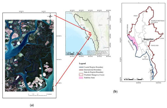
Figure 1.
Location of the study area, (a) Wunbaik Mangrove Forest (Sentinel-2 true color image), (b) Rakhine coastal region in Myanmar.
2.2. Field Survey
Field surveys were conducted from 15 September to 10 October 2019 to acquire accurate and current information on the study area. The supervised classification required a reliable ground truth image to train the neural network model for mangrove classification. The study area contained abundant natural mangroves and various land-use types (Table 1). Therefore, the latitudes and longitudes of the ground truth points for each land-use type were collected using a handheld global positioning system (GPS) (GARMIN etrex 10), providing a horizontal accuracy of approximately 3 m. Figure 2 shows the locations of the ground truth points with matching photos taken in the field.

Table 1.
Ground location points of different land uses in the study area.
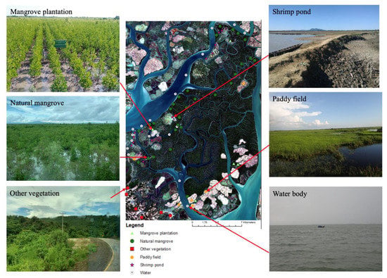
Figure 2.
Ground location points of different land covers of mangrove plantation, natural mangrove, other vegetation, shrimp pond, paddy field, and water body (Photos were taken by Win Sithu Maung during the field survey of this study).
2.3. Preparation of a Ground Truth Image
Preparing accurate ground truth data was necessary in supervised classification and was a major challenge for training and evaluating a neural network model. To obtain a reliable ground truth image, location points collected in the field were imported into ArcGIS. Polygons were manually drawn by referring to the same land cover of the ground truth points, using high-resolution Google Earth imagery and different combinations of Sentinel-2 satellite bands. For accurate mangrove recovery analysis, two major classes were assigned as mangrove and non-mangrove (rather than multi-classification, which may lead to massive time consumption for creating ground truth images). Assigned polygons were converted into a raster image with a resolution of 10 m. A ground truth image, which has assigned values of 0 and 255 for every pixel, was obtained. All 53,939,393 pixels, of which the ground truth image had a width and height of 1914 × 2814 pixels with a resolution of 10 m, were counted as the dataset for the ANN prediction.
To assess natural recovering mangroves in abandoned shrimp ponds and to ensure the identification of natural recovery sites, we set 3 criteria: (1) No planted mangroves, (2) same abandonment year, and (3) site accessibility. Three disused ponds, which met these criteria, were selected after discussions with the local staff of the Forest Department and the pond owners (Figure 3). The locations of these abandoned ponds were collected to create polygons of the recovered ponds. Recovering mangrove species at the selected abandoned sites were observed by conducting a field inventory in 50 sample plots with the assistance of knowledgeable local laborers and Forest Department staff (Figure 3).
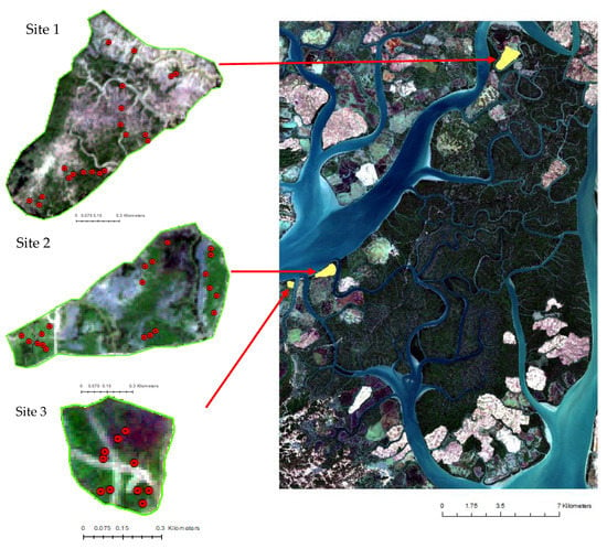
Figure 3.
Locations of three selected abandoned sites and sample plots.
2.4. Earth Observation Data
2.4.1. Satellite Band Information
To create the required datasets for the ANN classification, sets of multi-spectral bands of Sentinel-2 satellite imagery were collected from the Copernicus Open Access Hub using the semi-automatic classification plugin (SCP) in QGIS [53]. To detect changes in the mangroves and identify recovering mangrove areas within the selected abandoned sites, cloud-free Sentinel-2 images from 21 January 2020, and 23 December 2015 (during the dry seasons) were utilized. Detailed information regarding Sentinel-2 data acquisition is provided in Table 2.

Table 2.
Specification of Sentinel-2 products used in this study.
Currently, 2 major products of Sentinel-2 imagery (Level-1 C and Level-2 A) are disseminated to the public by the European Space Agency [54]. Level-1 C provides orthorectified Top-Of-Atmosphere reflectance, whereas Level-2 C, which was extended globally in December 2018, offers orthorectified Bottom-Of-Atmosphere reflectance. The spatial resolutions of multi-spectral bands provided by Sentinel-2 were 10, 20, and 60 m [55]. We used 10 Sentinel-2 spectral bands, excluding bands 1, 9, and 10, which had a poor spatial resolution of 60 m and were unrelated to the aim of mangrove classification. Sentinel-2 bands with various resolutions were resampled to a resolution of 10 m using the nearest neighbor algorithm for 2015 and 2020. As the multi-spectral bands acquired in 2015 were Level-1 C products, an atmospheric correction was conducted using the dark object subtraction 1 method provided in the SCP QGIS tool [53].
2.4.2. Spectral Indices
In addition to the multi-spectral bands of satellite images, spectral indices were one of the most effective features that offered information on land use and land cover. The normalized difference vegetation index (NDVI), normalized difference water index (NDWI), and combined mangrove recognition index (CMRI) were used as input features to train the neural network model. The NDVI was calculated using band 4 (RED) and band 8 (near infrared (NIR)) (Equation (1)) [56], whereas the NDWI was derived from Equation (2) using band 3 (GREEN) and band 8 (NIR) (Equation (2)) [57]. The CMRI was determined based on the difference between the NDVI and NDWI (Equation (3)) [58].
2.4.3. Digital Elevation Model
Collecting topographic data over the entire study area during the field survey was problematic because of difficulties in accessing the mangrove area. To overcome this challenge, we applied the SRTM for DSM and the MERIT DEM for DTM. During the SRTM mission in February 2000, the SRTM 1 arc second DEM was created from the C-band radar data acquired by the cooperation of the National Aeronautics and Space Administration and the National Geospatial-Intelligence Agency. The SRTM1 DEM provided user elevation values with a resolution of 30 m, referring to the WGS84 ellipsoid as a horizontal datum and the geoid as a vertical datum. It may be freely downloaded from the USGS EarthExplorer website (https://earthexplorer.usgs.gov/) [59]. The MERIT DEM was downloaded free of charge from the MERIT_DEM website (http://hydro.iis.u-tokyo.ac.jp/~yamadai/MERIT_DEM/).
2.4.4. Canopy Height Model
This study used canopy height information for the large-scale classification of mangrove extent. Applying the SRTM DEM as a DSM data source was reasonably acceptable in estimating forest height [60], and the MERIT DEM provided true topographic information. We ensured the reliability of the two DEMs by comparing field data collected during the post-processed kinematic (PPK) survey (Figure 4). The resulting CHM applied was derived from the difference between the SRTM DEM and MERIT DEM.
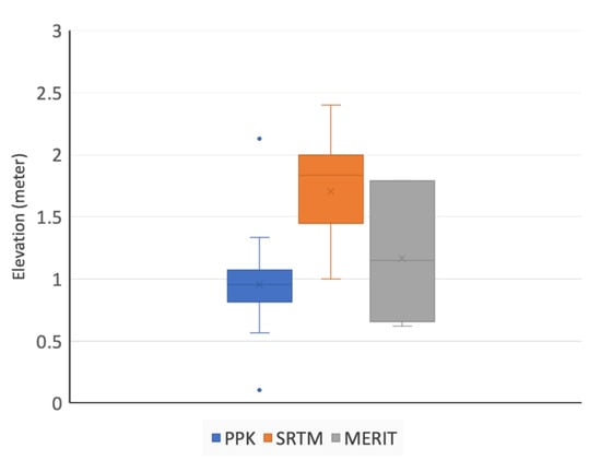
Figure 4.
Comparison of Shuttle Radar Topography Mission (SRTM) and Multi-Error-Removed-Improved-Terrains (MERIT DEMs) with post-processed kinematic (PPK) ground truth elevation data.
2.5. Artificial Neural Network Classification
An ANN model is based on the structure of the biological neural network of the human nervous system and primarily consists of a multi-layer perceptron with an input layer, a hidden layer, an output layer, and interconnected operating nodes similar to brain nerve cells in each layer [61]. The nodes in the input layer transfer feature values (), weight information (), and bias () from a dataset to the hidden layer. In the hidden layer, data obtained from the input layer are analyzed through an activation function in each node, and the generated data () are conveyed to the output layer (Equation (4)).
Based on the basic model architecture, the ANN model for this study was first created with 1 hidden layer and 12 neurons as a basic model using a sequential model of the Keras Application Programming Interface (https://keras.io/api/models/) and TensorFlow 2.3.0 (https://www.tensorflow.org/api_docs/python/tf/keras/sequential). We explored input features and hyper-parameter tunings, where multiple experiments were conducted to obtain the most suitable combination of input features for mangrove classification. An optimum ANN model design was established by tuning the number of hidden layers and neurons. In terms of the activation functions that analyze input data within the neural network process, a rectified linear unit (ReLU) was applied to the hidden layers, and the Softmax function for the output layer. The ReLU function produced linear values for input data values larger than 0 and negative values for 0 (Equation (5)). The Softmax function [62,63] normalized the output value ranging from 0–1 and yielded the input value probability belonging to a particular class by dividing the summation (Equation (6)).
2.6. Workflow of Assessment of Natural Recovering Mangrove
Figure 5 illustrates the workflow of this research, which contained 3 primary approaches: (1) Input feature selection and hyper-parameter tuning for ANN classification; (2) application of a trained model to a new dataset and improvement of model performance through the transfer learning method; and (3) post-classification change detection. To delineate information on naturally recovering mangroves, the 3 abandoned sites were extracted from the mangrove change detection results. A detailed explanation of each process is provided in the following sections.
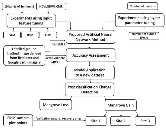
Figure 5.
Workflow of assessment of natural recovering mangrove at different abandoned sites.
2.6.1. Experimental Analysis through Input Feature and Hyper-Parameter Tuning
To select the most appropriate input feature combination for mangrove classification, different experimental classifications were first conducted using the basic ANN model. The raster images of the input features, multi-spectral satellite images of 10 bands, NDVI, NDWI, MERIT DEM, SRTM DEM, CHM, and ground truth images were converted into numerical datasets. Fifteen datasets were created and divided into 3 parts: Training data (60%), testing data (20%), and validation data (20%). This division was performed using the pre-processing modules of the scikit-learn data processing library (https://scikit-learn.org/stable/). The training dataset was applied to teach the ANN model by referring to the labeled data of the ground truth image, and the validation dataset was used to observe the behavior of the model to check for overfitting problems in every epoch of the training session simultaneously. The model was trained using the training dataset with 30 epochs for all experiments, and the trained model was applied to predict the testing dataset. Model performance was evaluated through overall accuracy and the kappa index.
After classification was completed using the trained model, the output datasets were exported in a raster format containing geographic information. The output raster images were visually assessed using true color Sentinel-2 and high-resolution Google Earth imagery in ArcGIS. Using the same approach, all datasets were analyzed to select a combination of input features, allowing the highest accuracy and a high-quality output map for mangrove classification.
Following the acquisition of the most suitable combination input features, the basic model was tuned in terms of the number of hidden layers and neurons. By adding one hidden layer to the basic model, the performance of each model was evaluated through accuracy and loss reduction, and a suitable number of hidden layers were selected. The number of neurons was then doubled in the hidden layers of the selected model to optimize the design of the ANN model.
2.6.2. Model Application to a New Dataset Using Transfer Learning
One of the advantages of neural network classification is that once the model is established with the desired accuracy, related new datasets can be predicted without re-training the model. After classifying the 2020 dataset through input features and hyper-parameter tuning, the trained ANN model was applied to a new dataset of the same input features for 2015.
Transfer learning is an emerging technique of machine learning in which a model trained for a given problem can theoretically be applied to a different yet related problem [64]. The performance of the pre-trained model may vary depending on the variation of input features of a new dataset, such as the spectral signatures of remotely sensed data acquired in different seasons. Retraining a model whenever a new problem is confronted in future predictions is a very time-consuming practice. To overcome such problems, transfer learning has become a practical and effective method for neural network classification. In this study, different layers of the original model were experimentally frozen and retrained to predict the new dataset.
During transfer learning, a new ground truth image was created by manually digitizing based on Google Earth images in 2015. 80% of the new dataset with the corresponding reference image randomly selected as training data and 20% of the dataset was the validation data. After conducting transfer learning through different experiments, the entire new dataset in 2015 was also predicted by all models.
2.6.3. Accuracy Assessment
Accuracy assessment is one of the major phases in image classification used to evaluate model performance. In this study, 20% of the ground truth image was used for validation after training the model. Model performance was evaluated using the overall accuracy and kappa coefficient, the most widely used measure to assess the accuracy of satellite image classification [65]. For the new prediction in 2015 using the ANN model trained with the 2020 dataset, 1000 reference points with geographic locations and land cover information were randomly generated to represent the entire study area. The predicted points were then extracted from the classified images from 2015, and model performance was assessed by comparing them with the reference points.
A confusion or error matrix representing the ground truth pixels in the column and classified pixels in the row for each class was created to assess the classification accuracy. The overall accuracy was then calculated by dividing the sum of truly classified pixels of each class by the total number of pixels in the diagonal elements of the confusion matrix. The kappa coefficient, precision, recall, and F1 score were also used, as they considered the true positive pixels, the false-negative pixels, and the non-diagonal elements in a confusion matrix [66,67]. These parameters ranged from 0 to 1; values closer to 1 denoted higher classification accuracy.
2.6.4. Post-Classification Change Detection
Acquiring accurate information on changes to the mangroves is critical for mangrove conservation, to determine past occurrences, implement future restoration programs, and develop the necessary regulations [68]. Among the various available change detection methods, pixel-to-pixel-based post-classification change detection was used in this study to provide promising classification accuracy results [69]. The 2 classified images in 2015 and 2020 were differentiated in the post-classification change detection analysis. Areas that underwent extensive changes were highlighted to identify the primary drivers of mangrove dynamics. Using Sentinel-2 and high-resolution Google Earth imagery, the findings were visually clarified to understand the causes of these changes.
2.6.5. Assessment of Natural Recovering Mangroves at Different Abandoned Sites
Based on the post-classification change detection results, 3 selected sites were extracted from the mangrove gain areas to identify naturally recovering mangroves for different abandoned shrimp ponds. Naturally recovering areas at t3 selected sites were quantified in ArcGIS, and the capacity of natural recovery was compared with the extent of the ponds.
3. Results
3.1. Artificial Neural Network Classification
3.1.1. Experimental Results of Input Feature Selection
Using the basic ANN model, 15 experiments using various combinations of input features were conducted to identify the 2020 mangrove distribution of the WMF. Different levels of accuracy were obtained depending on the input feature combination in each experiment (Table 3). Experiment 1 using 10 bands of the Sentinel-2 satellite image produced an unsatisfactory accuracy of 56.39%, revealing that the use of only spectral information from satellite bands was insufficient to classify mangrove distribution using the ANN model. As such, Experiment 1 was not adopted to produce an output image of the classification result because of its poor accuracy.

Table 3.
Experimental results of input feature adjustment.
Based on the outcomes of Experiment 1, more informative input features were required in the classification; two spectral indices of NDVI and NDWI were included in Experiment 2. After implementing the same procedures, a relatively higher accuracy of 93.43% was achieved in Experiment 2. Despite the satisfactory accuracy in Experiment 2, the output image showed that this combination of input features was still incapable of distinguishing mangroves from other types of vegetation (Figure 6c). To undertake this differentiation, a newly developed index, CMRI, was applied in Experiment 3. The resultant accuracy was improved to 94.02%; however, there were no effective changes in terms of the determination of other vegetation types (Figure 6d).
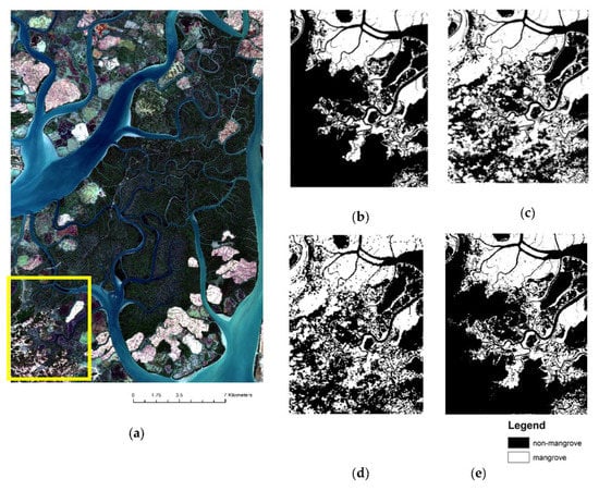
Figure 6.
(a)The study area (Sentinel-2 true color image) and mixed vegetation area in (b) ground truth image, classified images of (c) Experiment 2, (d) Experiment 3, and (e) Experiment 6.
In Experiment 4, topographic information was utilized (instead of CMRI), as most of the other vegetation in the study area thrives in the upper land area. Therefore, the MERIT DEM was applied to Experiment 4 in an effort to remove the misclassified pixels of other vegetation types. Following Experiment 4, the other forested areas misclassified as mangrove vegetation in the previous experiments could be converted into non-mangrove areas with an overall accuracy of 95.49% (Figure 6e). However, noisy and coarse pixels were still present in the mixed vegetation areas of the output image, potentially impacting classification accuracy due to the 90 m spatial resolution of the MERIT DEM.
We attempted to delineate the classification of mangrove distribution by applying the CHM derived from the SRTM DSM and MERIT DTM. After implementing different combinations of the DTM, DSM, and CHM in Experiments 6–9, the resultant accuracy was 95.85% in Experiment 6. Here, the DTM and CHM were integrated with the Sentinel-2 bands, NDVI, and NDWI. Furthermore, Experiment 6 eliminated noisy pixels from the output image in Experiment 4, producing a smooth map of the mangrove distribution. After implementing different classifications by adjusting input features, Experiment 6—containing 10 bands of the Sentinel-2 image, NDVI, NDWI, MERIT DEM, and CHM—produced the highest accuracy and the best delineation for mangrove distribution of the 15 experiments (Figure 7c). Other than experiments 1, 2, 3, 4, and 6, the results of the remaining experiments were excluded from this study because these experiments were tested with minor changes in input features and demonstrated no outperformance in mangrove classification. The accuracies of all the experiments are provided in Table 3.
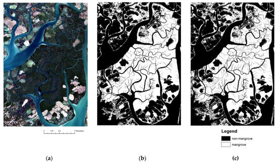
Figure 7.
(a) Sentinel-2 true color image, (b) ground truthed image, and (c) classified image of Experiment 6 of the whole study area.
3.1.2. Experimental Results of Hyper-Parameter Tuning
Using the dataset in Experiment 6 described in the input parameter tuning section, hyper-parameter tuning was evaluated by adjusting the number of hidden layers and neurons. First, one hidden layer with 10 neurons was added to the basic model used in the input feature adjustment. The model trained and evaluated the accuracy while visually checking the behavior of the model in the accuracy learning curves and loss using the validation dataset. Following the addition of up to four hidden layers, the model with two hidden layers (12:10) produced the highest accuracy of 95.89%. The accuracy of the model with three hidden layers (12:10:8) and four hidden layers (12:10:10:8) was the same at 95.76% (Figure 8).
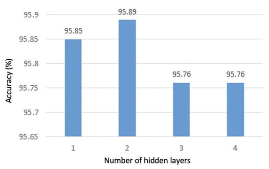
Figure 8.
Evaluation results of artificial neural network (ANN) models with different hidden layers.
To evaluate model behavior, the accuracy and loss of training were compared to those of the validation prediction. Figure 9a shows that the loss reduction of the training prediction of the model with two hidden layers was less divergent and had a direction similar to the validation at the end of the learning curve. In contrast, the models with three and four hidden layers showed greater differences between training and validation measures and were overfitted; validation losses significantly increased at the end of learning despite the stable declining trend in training (Figure 9b,c). Thus, the model with two hidden layers was selected based on evaluating the classification accuracy and model behavior during the learning time.

Figure 9.
Learning curves of loss reduction of model with (a) two hidden layers, (b) three hidden layers, and (c) four hidden layers during the training phase.
The neurons in the hidden layers played a key role as processing units in analyzing input data and producing output; hence, the number of neurons influences the performance of the ANN model. The number of neurons in the two selected hidden layers was adjusted by halving and doubling the neurons in each layer to test the performance. Comparing the accuracy and loss of training prediction to that of validation in each model, the model with greater neurons (544:320) performed with the highest accuracy (95.98%), least error, and the smallest difference between the training and validation predictions (see Figure 10). After performing input features and hyperparameter tuning, the ANN model with two hidden layers (544:320 neurons) was selected as the model for mangrove classification using the input features of Experiment 6 (Figure 11).
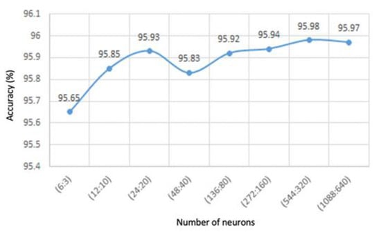
Figure 10.
Model accuracy depending on the number of neurons in hidden layers.
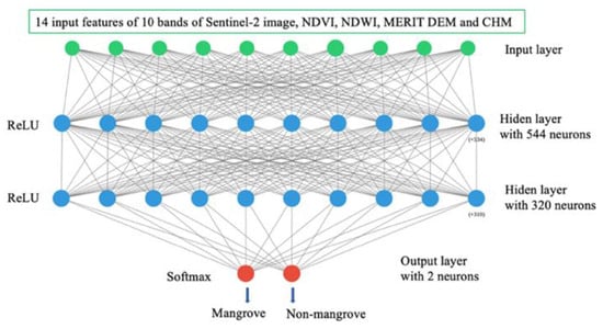
Figure 11.
Proposed ANN model and input dataset for classification of mangrove distribution.
3.2. Classification Results of New Prediction Using Transfer Learning
The ANN model with two hidden layers (544:320), obtained through hyper-parameter tuning, was applied to a new dataset from 2015, with the same input features. The model produced an overall accuracy of 94.50% and a kappa coefficient of 0.92. Despite the high classification accuracy, the model falsely classified green paddy fields as mangroves in the new prediction due to the spectral variation in different seasons. To overcome this problem, certain parameters of the original model were fixed with existing knowledge, whereas others were retrained with a new dataset that contained information on the green paddy fields (Figure 12).
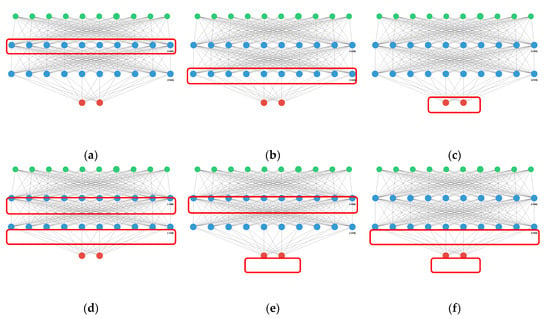
Figure 12.
Six different types of models in transfer learning process: (a) T0 model fixed layer 0, (b) T1 model fixed layer 1, (c) T2 model fixed layer 2, (d) T01 model fixed layer 0 and 1, (e) T02 model fixed layer 0 and 2, and (f) T12 model fixed layer 1 and 2.
The classification results of the experiments are listed in Table 4. The original model produced a low accuracy of 72.59% for the transfer learning dataset owing to the spectral variation problem in the paddy fields. The original model was tested with different layer fixing and re-training settings. Of the six different models re-trained in transfer learning, the T12 model, which fixed the second hidden layer (layer 1) and output layer (layer 2), could be trained within the shortest training time of 32 s per epoch (using one node on the supercomputer ITO-B at Kyushu University). The T12 model also outperformed the other models, obtaining the highest accuracy of 97.2% and a kappa coefficient of 0.94 for the whole dataset, and a high accuracy of 95.77% for the transfer learning dataset. As a result, the T12 model could eliminate misclassified paddy field pixels predicted by the original model (see Figure 13c). After conducting mangrove classifications using the ANN model in 2020 and 2015, the validation parameters obtained in this study are described in Table 5; the final mangrove distribution maps of the two periods are shown in Figure 14.

Table 4.
Classification results of different models in transfer learning.
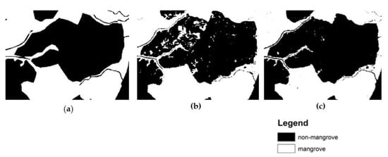
Figure 13.
(a) Reference image of green paddy field area in 2015 dataset, (b) classified image of the original model and (c) classified image of T12 model.

Table 5.
Accuracy, kappa, precision, recall, and F1 scores and statistical significance (Z-test) assessment of ANN model for mangrove classification.
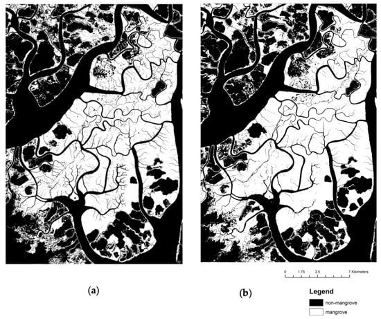
Figure 14.
Mangrove distribution maps of Wunbaik Mangrove Forest in (a) 2020 and (b) 2015 predicted by the proposed ANN method.
Moreover, the statistical significance of the overall accuracies of the two classifications in 2020 and 2015 was assessed using Z-test [70], and the resultant Z-value and p-value were 0.4753 and 0.63122, respectively (Table 5). The difference in classification accuracies of the two periods was not statistically significant because the proposed method could achieve high accuracies in both classifications of 2020 and 2015 despite the slight improvement in the 2015 classification.
3.3. Mangrove Changes and Drivers
To provide updated information on the mangrove distribution in the WMF, we examined spatial changes in mangroves between 2015 and 2020. By differentiating between classified images in 2015 and 2020, the change detection results showed significant changes in mangrove extent in the WMF (Figure 15a). To focus on the major causes of mangrove loss and gain, only extensive change areas were examined and validated with Sentinel-2 true color imagery (10 m resolution) and very high resolution (1 m) Google Earth imagery.
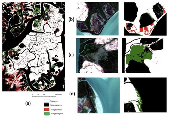
Figure 15.
(a) Change detection result of Wunbaik Mangrove Forest (WMF), (b) Mangrove loss area due to shrimp pond expansion, (c) Mangrove gain area in artificial plantation, and (d) Mangrove gain area through natural regeneration.
Interpreting change detection results based on field information and mangrove losses in the study area between 2015 and 2020 was warranted because of the expansion of shrimp ponds (Figure 15b), whereas mangrove gain patches were detected at plantation sites (Figure 15c) and naturally regenerated areas (Figure 15d). The locations of artificial mangrove plantations established by the Forest Department were identified using high-resolution Google Earth imagery and GPS points collected during the field survey. Naturally recovered mangroves were found in active shrimp ponds, abandoned sites, and tidal flats. Between 2015 and 2020, the total mangrove area declined from 254.30–249.83 km2 slightly, whereas the non-mangrove area increased from 284.30–288.77 km2.
3.4. Natural Recovery of Mangroves at Abandoned Sites
To delineate the naturally recovering mangroves in the study area, three abandoned shrimp ponds selected during the field survey were extracted from the results of change detection. The recovering mangrove area in each abandoned pond was then evaluated and compared to the extent of the abandoned sites in ArcGIS. During the abandonment period from 2015 to 2020, mangrove cover increased by 49.02% at Site 1, 55.93% at Site 2, and 50.00% at Site 3 (Table 6). The results showed that mangroves could naturally recover in approximately half of the abandoned sites without any artificial effort (Figure 16).

Table 6.
Naturally recovering percentage of mangrove at different abandoned shrimp ponds.
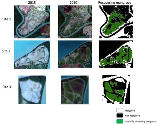
Figure 16.
Naturally recovering mangrove at different abandoned sites between 2015 and 2020.
The field survey and collaboration with Forest Department staff and shrimp pond owners confirmed that there was no artificial planting following the abandonment of these shrimp ponds. The recovering mangrove areas were validated using ground truth GPS points of 50 sample plots collected from the 3 recovery sites, and 12 different mangrove species were identified through the field inventory. Avicennia officinalis (Figure 17a) was the dominant species at Site 1, whereas A. marina (Figure 17b,c) dominated at sites 2 and 3.
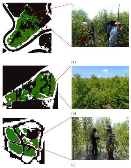
Figure 17.
Ground checked photos of naturally recovering mangrove species at (a) Site 1 dominating Avicennia officinalis, (b) Site 2, and (c) Site 3 dominating Avicennia marina.
4. Discussion
The nature of mangrove intertidal ecosystems characterized by mixing with other vegetation in adjacent parts creates many challenges for the classification of mangrove distribution to produce accurate maps [14,41]. Selecting the most appropriate method in remote sensing analysis and an effective combination of input features is critical to overcoming such complex issues. Apart from the complex features of mangrove forests, different classification methods also have various drawbacks. In another analysis, Chun et al. compared the ANN method with the maximum likelihood classifier using Thailand Earth Observation System (THEOS) satellite data for mangrove mapping [44]. The study conducted by Toosi et al. on mangrove forest cover changes produced high overall accuracy (ranging 81–93%) by comparing machine learning algorithms (RF, RDA, and SVM) [17]. This study explored the ANN approach using Sentinel-2 satellite imagery for mangrove classification through various experiments with input features and hyper-parameter tuning.
The incorporation of topographic features in remote sensing classification generated a favorable outcome for mangrove mapping in other studies [71,72]. However, obtaining true topographic information remains challenging. This study integrated topographic information derived from the MERIT DEM to achieve high accuracy classification and to eliminate misclassified pixels from previous experiments. Despite these merits, the poor resolution of the MERIT DEM affected the quality of the output map with many noisy pixels.
The resulting accuracy of tree species classification was improved by applying the CHM derived from the differentiation of the DTM and DSM. The CHM obtained from multi-spectral and hyperspectral images and Light Detection and Ranging (LiDAR) data have been applied for mangrove species classification [73,74]. Cao et al. [28] showed that the CHM generated from a hyperspectral sensor mounted on a UAV was useful for mangrove species discrimination. However, owing to limited accessibility and the high investment involved with LiDAR, SAR data, and hyperspectral sensors, such as canopy height collection methods, are rarely deployed in remote sensing classification [75]. This study attempted to employ the CHM obtained from the freely and globally accessible SRTM DSM and MERIT DEM for mangrove classification. We found that mangrove distribution may be more accurately identified by integrating the DTM and CHM in remote sensing classification. Classification accuracy and image quality could improve future mangrove distribution mapping if the CHM was derived from higher resolution and more accurate DTM and DSM.
For the ANN model, a universal method to select the number of hidden layers and neurons for optimal model design is lacking [76,77]. Thus, a systematic experimental analysis presents a reliable path for solving a specific problem [78]. After conducting hyper-parameter tuning, the selected model with two hidden layers (544:322) outperformed the other models, obtaining the highest accuracy of 95.98%, whereas the basic model obtained an accuracy of 95.85% with the same dataset. The results of the analyses show that the setting of the deployed method is one of the pivotal factors in remote sensing classification, as it influences the selection of efficient input features. Although there were no dramatic improvements in accuracy, the behavior of the models was considered through the validation dataset to avoid overfitting problems for future predictions.
By developing advanced technologies in computer science, the remote sensing community has improved many classification methods by applying a state-of-the-art approach for time and cost-effective computation. Transfer learning is a cutting edge approach in neural networks and effective for future predictions through the use of a relatively small training dataset with reduced computational costs [79,80,81]. Guo [82] introduced and applied transfer learning to identify buildings in rural environments. This study confronted issues with the misclassification of green paddy fields by the trained model. Transfer learning was employed by delineating different layers of frozen data to overcome this issue. The original model was leveraged by re-training one hidden layer with a very small dataset. The resulting accuracy for the entire study area significantly improved from 94.50–97.20%. Through transfer learning, we built the model to be more applicable for mangrove classification in different seasons and regions. Despite satisfactory classification accuracy results, preparing a ground truth image to create a large amount of training data and a long-running time for ANN prediction limit the proposed approach. Moreover, our study has some uncertainties, as we could not apply a ground truth image to validate the performance of the pretrained ANN model in the 2015 classification. To address this necessity, we applied a reference image digitized using Google Earth imagery. Considering this limitation, future studies should explore the variable importance of highlighting the contributions of each variable in ANN classification for mangrove distribution.
Mangrove forests in Myanmar have declined, with an annual net reduction rate of 3.60–3.87% between 1996 and 2016, because of competition with and expansion of agricultural fields, aquaculture, palm oil, and rubber [83,84]. FAO [8] and Aye Saw [85] studied mangrove forest changes in WRMF and described shrimp ponds and paddy fields as the primary drivers of mangrove loss between 1990 and 2011, and 1990 to 2014, respectively. Similarly, this study observed that the mangrove area of WMF in 2015 declined slightly in 2020. The reason for mangrove loss was largely due to the expansion of shrimp ponds by local communities, whereas mangrove forests were able to expand by artificial plantation and natural recovery processes. Interestingly, the change detection results showed that more mangrove loss areas were discovered near local villages due to the expansion of shrimp farming than within the reserved forest (Figure 18).
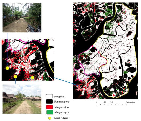
Figure 18.
Shrimp pond expansion by local villages near the WRMF between 2015 and 2020.
One of the uncertainties is that the study could not distinguish shrub, planted, and natural recovering mangrove due to the medium resolution of the Sentinel-2 satellite images. A 10 m pixel range might include real shrub and weeds other than mangrove species, and high-resolution satellite or UAV images should be applied to validate mangrove classification and to change detection results. However, the only mangrove restoration projects in WMF are artificial plantations established by the Forest Department; other mangrove gain areas were assumed to appear as a result of natural recovery processes. Although recovering mangroves were also found in the active shrimp ponds of the WMF, the long-term survival of these mangroves is questionable, as they would likely be cleared if the owners wanted to repair their shrimp ponds or if the ponds were converted to paddy fields. However, these results highlight the natural recovery process in abandoned areas. The results show that mangroves are able to naturally recover in approximately 50% of the abandoned sites with a diverse range of species within a short period of abandonment from 2015 to 2020.
5. Conclusions
This study was the first attempt to employ the ANN classification using Sentinel-2 imagery for mangrove classification. We conducted two primary experiments relating to input features and hyper-parameter tuning. Based on these experiments, we proposed a promising ANN model applying Sentinel-2 satellite imagery and topographic and canopy height information for constraining mangrove distribution. Through optimization, we achieved the highest overall accuracy of 95.98%, a kappa coefficient of 0.92, mangrove and non-mangrove precisions of 0.95 and 0.98, respectively, recalls of 0.96, and F1 scores of 0.96. Moreover, we used the transfer learning approach to improve the ANN model performance and obtained a high overall accuracy of 97.20%, a kappa coefficient of 0.94, mangrove and non-mangrove precisions of 0.98 and 0.96, respectively, recalls of 0.98 and 0.97, and F1 scores of 0.96. The created model can be deployed for mangrove classification in different seasons and regions.
The outcomes of this study contribute to the production of up-to-date and reliable information regarding mangrove change in the WMF through post-classification change detection. The results highlight that the mangrove extent decreased in the WMF between 2015 and 2020, owing to the expansion of shrimp ponds. By integrating field observations with the change detection results, we highlight that the mangroves were able to naturally recover in approximately 50% of the abandoned sites within a short abandonment period. Further research on the natural recovery process of mangroves should be conducted, as it presents a valuable opportunity for mangrove rehabilitation after human disturbance.
Author Contributions
W.S.M. is responsible for this study. W.S.M. conducted a field survey and analyzed the preprocessing and main experiments. W.S.M. prepared the original draft manuscript. J.S. supervised the study, collaborated the field survey, provided a careful review and editing to the manuscript, and contributed to funding acquisition. All authors have read and agreed to the published version of the manuscript.
Funding
This research was partially funded by JSPS KAKENHI Grant Number JP20H02250.
Acknowledgments
The ANN computation was performed using the computer resources offered under the category of General Projects by the Research Institute for Information Technology, Kyushu University. We are thankful to Dai Yamzaki, Institute of Industrial Science, The University of Tokyo, for providing the MERIT DEM. The first author is deeply indebted to the Asian Development Bank for financial support during the study period in Japan. The authors would like to express our gratitude to the anonymous reviewers for careful reading of our manuscript and their insightful comments and suggestions.
Conflicts of Interest
The authors declare no conflict of interest.
References
- Spalding, M. World Atlas of Mangroves; Routledge: Abingdon-on-Thames, UK, 2010. [Google Scholar]
- Brander, L.M.; Wagtendonk, A.J.; Hussain, S.S.; McVittie, A.; Verburg, P.H.; De Groot, R.S.; Van Der Ploeg, S. Ecosystem service values for mangroves in Southeast Asia: A meta-analysis and value transfer application. Ecosyst. Serv. 2012, 1, 62–69. [Google Scholar] [CrossRef]
- Alongi, D.M. Present state and future of the world’s mangrove forests. Environ. Conserv. 2002, 29, 331–349. [Google Scholar] [CrossRef]
- Richards, D.R.; Friess, D.A. Rates and drivers of mangrove deforestation in Southeast Asia, 2000–2012. Proc. Natl. Acad. Sci. USA 2016, 113, 344–349. [Google Scholar] [CrossRef]
- Veettil, B.K.; Pereira, S.F.R.; Quang, N.X. Rapidly diminishing mangrove forests in Myanmar (Burma): A review. Hydrobiologia 2018, 822, 19–35. [Google Scholar] [CrossRef]
- Lewis, R.R. Ecological engineering for successful management and restoration of mangrove forests. Ecol. Eng. 2005, 24, 403–418. [Google Scholar] [CrossRef]
- Kamali, B.; Hashim, R. Mangrove restoration without planting. Ecol. Eng. 2011, 37, 387–391. [Google Scholar] [CrossRef]
- Stanley, D.O.; Broadhead, J.; Aung Aung, M.; Burma. Forest Department; Food and Agriculture Organization of the United Nations. The Atlas and Guidelines for Mangrove Management in Wunbaik Reserved Forest; FAO-UN, Seed Division Compound, Insein Road, Yangon, Myanmar Publications: Yangon, Myanmar, 2011; Volume iii, 132p. [Google Scholar]
- Giri, C. Observation and monitoring of mangrove forests using remote sensing: Opportunities and challenges. Remote Sens. 2016, 8, 783. [Google Scholar] [CrossRef]
- Wang, L.; Jia, M.; Yin, D.; Tian, J. A review of remote sensing for mangrove forests: 1956–2018. Remote Sens. Environ. 2019, 231, 111223. [Google Scholar] [CrossRef]
- Yoshino, K.; Pham, T.D.; Bui, D.T.; Friess, D.A.; Yokoya, N.; Bui, D.T.; Yoshino, K.; Friess, D.A. Remote sensing approaches for monitoring mangrove species, structure, and biomass: Opportunities and challenges. Remote Sens. 2019, 11, 1–24. [Google Scholar]
- Lu, D.; Weng, Q. A survey of image classification methods and techniques for improving classification performance. Int. J. Remote Sens. 2007, 28, 823–870. [Google Scholar] [CrossRef]
- Ahmad, A.; Quegan, S. Comparative analysis of supervised and unsupervised classification on multispectral data. Appl. Math. Sci. 2013, 7, 3681–3694. [Google Scholar] [CrossRef]
- Green, E.P.; Clark, C.D.; Mumby, P.J.; Edwards, A.J.; Ellis, A.C. Remote sensing techniques for mangrove mapping. Int. J. Remote Sens. 1998, 19, 935–956. [Google Scholar] [CrossRef]
- Rahman, M.; Ullah, R.; Lan, M.; Sri Sumantyo, J.T.; Kuze, H.; Tateishi, R. Comparison of Landsat image classification methods for detecting mangrove forests in Sundarbans. Int. J. Remote Sens. 2013, 34, 1041–1056. [Google Scholar] [CrossRef]
- Nguyen, H.H.; Nghia, N.H.; Nguyen, H.T.T.; Le, A.T.; Tran, L.T.N.; Duong, L.V.K.; Bohm, S.; Furniss, M.J. Classification methods for mapping mangrove extents and drivers of change in Thanh Hoa province, Vietnam during 2005–2018. For. Soc. 2020, 4, 225–242. [Google Scholar] [CrossRef]
- Toosi, N.B.; Soffianian, A.R.; Fakheran, S.; Pourmanafi, S.; Ginzler, C.; Waser, L.T. Comparing different classification algorithms for monitoring mangrove cover changes in southern Iran. Glob. Ecol. Conserv. 2019, 19. [Google Scholar] [CrossRef]
- Kamal, M.; Jamaluddin, I.; Parela, A.; Farda, N.M. Comparison of Google Earth Engine (GEE)-based machine learning classifiers for mangrove mapping. In Proceedings of the 40th Asian Conference Remote Sensing, ACRS 2019, Daejeon, Korea, 14–18 October 2019; Volume 2000, pp. 1–8. [Google Scholar]
- Campomanes, F.; Pada, A.V.; Silapan, J. Mangrove classification using support vector machines and random forest algorithm: A comparative study. In Proceedings of the GEOBIA 2016—Solutions & Synergies, Enschede, The Netherlands, 14–16 July 2016; pp. 2–6. [Google Scholar]
- Altaei, M.S.M. Satellite Image Classification Using Artificial Neural Network. Int. J. Res. Advent Technol. 2019, 7, 459–462. [Google Scholar]
- Toshniwal, M. Satellite image classification using neural networks. In Proceedings of the Third International Conference on Sciences of Electronic, Technology of Information and Telecommunications (SETIT 2005), Susa, Tunisia, 17–21 March 2005; pp. 1–5. [Google Scholar]
- Ge, G.; Shi, Z.; Zhu, Y.; Yang, X.; Hao, Y. Land use/cover classification in an arid desert-oasis mosaic landscape of China using remote sensed imagery: Performance assessment of four machine learning algorithms. Glob. Ecol. Conserv. 2020, 22, e00971. [Google Scholar] [CrossRef]
- Kawabata, D.; Bandibas, J. Landslide susceptibility mapping using geological data, a DEM from ASTER images and an Artificial Neural Network (ANN). Geomorphology 2009, 113, 97–109. [Google Scholar] [CrossRef]
- Wang, L.; Sousa, W.P.; Gong, P.; Biging, G.S. Com. Remote Sens. Environ. 2004, 91, 432–440. [Google Scholar] [CrossRef]
- Xia, J.; Yokoya, N.; Pham, T.D. Probabilistic mangrove species mapping with multiple-source remote-sensing datasets using label distribution learning in Xuan Thuy National Park, Vietnam. Remote Sens. 2020, 12, 3834. [Google Scholar] [CrossRef]
- Poortinga, A.; Tenneson, K.; Shapiro, A.; Nquyen, Q.; Aung, K.S.; Chishtie, F.; Saah, D. Mapping plantations in Myanmar by fusing Landsat-8, Sentinel-2 and Sentinel-1 data along with systematic error quantification. Remote Sens. 2019, 11, 831. [Google Scholar] [CrossRef]
- Li, Q.; Wong, F.K.K.; Fung, T. Classification of mangrove species using combined WordView-3 and LiDAR data in Mai Po Nature Reserve, Hong Kong. Remote Sens. 2019, 11, 2114. [Google Scholar] [CrossRef]
- Cao, J.; Leng, W.; Liu, K.; Liu, L.; He, Z.; Zhu, Y. Object-Based mangrove species classification using unmanned aerial vehicle hyperspectral images and digital surface models. Remote Sens. 2018, 10, 89. [Google Scholar] [CrossRef]
- European Space Agency ESA—About the Launch. Available online: https://www.esa.int/Applications/Observing_the_Earth/Copernicus/Sentinel-2/About_the_launch (accessed on 30 June 2020).
- Astola, H.; Häme, T.; Sirro, L.; Molinier, M.; Kilpi, J. Comparison of Sentinel-2 and Landsat 8 imagery for forest variable prediction in boreal region. Remote Sens. Environ. 2019, 223, 257–273. [Google Scholar] [CrossRef]
- García-Llamas, P.; Suárez-Seoane, S.; Fernández-Guisuraga, J.M.; Fernández-García, V.; Fernández-Manso, A.; Quintano, C.; Taboada, A.; Marcos, E.; Calvo, L. Evaluation and comparison of Landsat 8, Sentinel-2 and Deimos-1 remote sensing indices for assessing burn severity in Mediterranean fire-prone ecosystems. Int. J. Appl. Earth Obs. Geoinf. 2019, 80, 137–144. [Google Scholar] [CrossRef]
- Lima, T.A.; Beuchle, R.; Langner, A.; Grecchi, R.C.; Griess, V.C.; Achard, F. Comparing Sentinel-2 MSI and Landsat 8 OLI Imagery for Monitoring Selective Logging in the Brazilian Amazon. Remote Sens. 2019, 11, 961. [Google Scholar] [CrossRef]
- Connette, G.; Oswald, P.; Songer, M.; Leimgruber, P. Mapping distinct forest types improves overall forest identification based on multi-spectral landsat imagery for Myanmar’S Tanintharyi Region. Remote Sens. 2016, 8, 882. [Google Scholar] [CrossRef]
- Ha, N.T.; Manley-Harris, M.; Pham, T.D.; Hawes, I. A comparative assessment of ensemble-based machine learning and maximum likelihood methods for mapping seagrass using sentinel-2 imagery in Tauranga Harbor, New Zealand. Remote Sens. 2020, 12, 355. [Google Scholar] [CrossRef]
- Morgan, R.S.; El-Hady, M.A.; Rahim, I.S. Soil salinity mapping utilizing sentinel-2 and neural networks. Indian J. Agric. Res. 2018, 52, 524–529. [Google Scholar]
- Mohite, J.; Twarakavi, N.; Pappula, S. Evaluating the Potential of Sentinel-2 for Low Severity Mites Infestation Detection in Grapes. In Proceedings of the 2018 IEEE International Geoscience and Remote Sensing Symposium, IGARSS 2018, Valencia, Spain, 22–27 July 2018; pp. 4651–4654. [Google Scholar]
- Pereira-Pires, J.E.; Aubard, V.; Ribeiro, R.A.; Fonseca, J.M.; Silva, J.M.N.; Mora, A. Semi-automatic methodology for fire break maintenance operations detection with sentinel-2 imagery and artificial neural network. Remote Sens. 2020, 12, 909. [Google Scholar] [CrossRef]
- Kristollari, V.; Karathanassi, V. Artificial neural networks for cloud masking of Sentinel-2 ocean images with noise and sunglint. Int. J. Remote Sens. 2020, 41, 4102–4135. [Google Scholar] [CrossRef]
- Lee, Y.S.; Lee, S.; Jung, H.S. Mapping forest vertical structure in Gong-Ju, Korea using sentinel-2 satellite images and artificial neural networks. Appl. Sci. 2020, 10, 1666. [Google Scholar] [CrossRef]
- Mondal, P.; Liu, X.; Fatoyinbo, T.E.; Lagomasino, D. Evaluating combinations of sentinel-2 data and machine-learning algorithms for mangrove mapping in West Africa. Remote Sens. 2019, 11, 2928. [Google Scholar] [CrossRef]
- Bihamta Toosi, N.; Soffianian, A.R.; Fakheran, S.; Pourmanafi, S.; Ginzler, C.; Waser, L.T. Land Cover Classification in Mangrove Ecosystems Based on VHR Satellite Data and Machine Learning—An Upscaling Approach. Remote Sens. 2020, 12, 2684. [Google Scholar] [CrossRef]
- Yu, X.; Shao, H.B.; Liu, X.H.; Zhao, D.Z. Applying neural network classification to obtain mangrove landscape characteristics for monitoring the travel environment quality on the Beihai Coast of Guangxi, P.R. China. Clean Soil Air Water 2010, 38, 289–295. [Google Scholar] [CrossRef]
- Chun, B.B.; Jafri, M.Z.M.; San, L.H. Mangrove mapping in Penang Island by using artificial neural network technique. In Proceedings of the 2011 IEEE Conference on Open Systems ICOS 2011, Langkawi, Malaysia, 25–28 September 2011; pp. 251–255. [Google Scholar]
- Chun, B.B.; Mat Jafri, M.Z.; San, L.H. Comparison of remote sensing approach for mangrove mapping over Penang Island. In Proceedings of the 4th International Conference on Computer and Communication Engineering 2012 (ICCCE 2012), Kuala Lumpur, Malaysia, 3–5 July 2012; pp. 258–262. [Google Scholar]
- Hutchinson, C.F. Techniques for combining Landsat and ancillary data for digital classification improvement. Photogramm. Eng. Remote Sens. 1982, 48, 123–130. [Google Scholar]
- Alganci, U.; Besol, B.; Sertel, E. Accuracy assessment of different digital surface models. ISPRS Int. J. Geo-Inf. 2018, 7, 114. [Google Scholar] [CrossRef]
- Lee, S.K.; Fatoyinbo, T.E. TanDEM-X Pol-InSAR Inversion for Mangrove Canopy Height Estimation. IEEE J. Sel. Top. Appl. Earth Obs. Remote Sens. 2015, 8, 3608–3618. [Google Scholar] [CrossRef]
- Wohlfart, C.; Winkler, K.; Wendleder, A.; Roth, A. TerraSAR-X and wetlands: A review. Remote Sens. 2018, 10, 916. [Google Scholar] [CrossRef]
- Ghosh, S.M.; Behera, M.D.; Paramanik, S. Canopy height estimation using sentinel series images through machine learning models in a Mangrove Forest. Remote Sens. 2020, 12, 1519. [Google Scholar] [CrossRef]
- Yamazaki, D.; Ikeshima, D.; Tawatari, R.; Yamaguchi, T.; O’Loughlin, F.; Neal, J.C.; Sampson, C.C.; Kanae, S.; Bates, P.D. A high-accuracy map of global terrain elevations. Geophys. Res. Lett. 2017, 44, 5844–5853. [Google Scholar] [CrossRef]
- Saw, A.A.; Kanzaki, M. Local Livelihoods and Encroachment into a Mangrove Forest Reserve: A Case Study of the Wunbaik Reserved Mangrove Forest, Myanmar. Procedia Environ. Sci. 2015, 28, 483–492. [Google Scholar] [CrossRef][Green Version]
- Win, M. The Mangrove Vegetation of Wubaik Reserved Forest; FAO-UN, Seed Division Compound, Insein Road, Yangon, Myanmar Publications: Yangon, Myanmar, 2011; Volume iii, 191p. [Google Scholar]
- Congedo, L. Semi-Automatic Classification Plugin Documentation; Lazio: Rome, Italy, 2016. [Google Scholar]
- Hościło, A.; Lewandowska, A. Mapping Forest Type and Tree Species on a Regional Scale Using Multi-Temporal Sentinel-2 Data. Remote Sens. 2019, 11, 929. [Google Scholar] [CrossRef]
- European Space Agency. SENTINEL-2 User Handbook; European Space Agency: Paris, France, 2015. [Google Scholar]
- Teillet, P.M.; Staenz, K.; Williams, D.J. Effects of spectral, spatial, and radiometric characteristics on remote sensing vegetation indices of forested regions. Remote Sens. Environ. 1997, 61, 139–149. [Google Scholar] [CrossRef]
- McFeeters, S.K. The use of the Normalized Difference Water Index (NDWI) in the delineation of open water features. Int. J. Remote Sens. 1996, 17, 1425–1432. [Google Scholar] [CrossRef]
- Gupta, K.; Mukhopadhyay, A.; Giri, S.; Chanda, A.; Datta Majumdar, S.; Samanta, S.; Mitra, D.; Samal, R.N.; Pattnaik, A.K.; Hazra, S. An index for discrimination of mangroves from non-mangroves using LANDSAT 8 OLI imagery. MethodsX 2018, 5, 1129–1139. [Google Scholar] [CrossRef]
- Yap, L.; Kandé, L.H.; Nouayou, R.; Kamguia, J.; Ngouh, N.A.; Makuate, M.B. Vertical accuracy evaluation of freely available latest high-resolution (30 m) global digital elevation models over Cameroon (Central Africa) with GPS/leveling ground control points. Int. J. Digit. Earth 2019, 12, 500–524. [Google Scholar] [CrossRef]
- Lee, W.J.; Lee, C.W. Forest canopy height estimation using multiplatform remote sensing dataset. J. Sens. 2018, 2018, 1–9. [Google Scholar] [CrossRef]
- Aggarwal, C.C. Neural Networks and Deep Learning; Gewerbestrasse 11: Cham, Switzerland, 2018; ISBN 9783319944623. [Google Scholar]
- Grave, E.; Joulin, A.; Cissé, M.; Grangier, D.; Jégou, H. Efficient softmax approximation for GPUs. In Proceedings of the 34th International Conference on Machine Learning (ICML 2017), Sydney, Australia, 6–11 August 2017; Volume 3, pp. 2111–2119. [Google Scholar]
- Uniqtech Understand the Softmax Function in Minutes—Data Science Bootcamp—Medium. Available online: https://medium.com/data-science-bootcamp/understand-the-softmax-function-in-minutes-f3a59641e86d (accessed on 15 June 2020).
- Pan, S.J.; Yang, Q. A survey on transfer learning. IEEE Trans. Knowl. Data Eng. 2010, 22, 1345–1359. [Google Scholar] [CrossRef]
- Rwanga, S.S.; Ndambuki, J.M. Accuracy Assessment of Land Use/Land Cover Classification Using Remote Sensing and GIS. Int. J. Geosci. 2017, 8, 611–622. [Google Scholar] [CrossRef]
- Congalton, R.G. Assessing Landsat Classification Accuracy Using Discrete Multivariate Analysis Statistical Techniques. Photogramm. Eng. Remote Sens. 1983, 49, 1671–1678. [Google Scholar]
- Cohen, J. A Coefficient of Aggrement for Normal Scales. Curr. Contents 1960, 20, 37–46. [Google Scholar]
- Gandhi, S.; Jones, T.G. Identifying mangrove deforestation hotspots in South Asia, Southeast Asia and Asia-Pacific. Remote Sens. 2019, 11, 728. [Google Scholar] [CrossRef]
- Afify, H.A. Evaluation of change detection techniques for monitoring land-cover changes: A case study in new Burg El-Arab area. Alex. Eng. J. 2011, 50, 187–195. [Google Scholar] [CrossRef]
- Glen, S. Z Test: Definition & Two Proportion Z-Test—Statistics How To. Available online: https://www.statisticshowto.com/z-test/ (accessed on 19 December 2020).
- Alsaaideh, B.; Al-Hanbali, A.; Tateishi, R.; Nguyen Thanh, H. The integration of spectral analyses of Landsat ETM+ with the DEM data for mapping mangrove forests. In Proceedings of the 2011 IEEE International Geoscience and Remote Sensing Symposium, Vancouver, BC, Canada, 24–29 July 2011; pp. 1914–1917. [Google Scholar]
- Alsaaideh, B.; Al-Hanbali, A.; Tateishi, R.; Kobayashi, T.; Hoan, N.T. Mangrove Forests Mapping in the Southern Part of Japan Using Landsat ETM+ with DEM. J. Geogr. Inf. Syst. 2013, 5, 369–377. [Google Scholar] [CrossRef]
- Chadwick, J. Integrated LiDAR and IKONOS multispectral imagery for mapping mangrove distribution and physical properties. Int. J. Remote Sens. 2011, 32, 6765–6781. [Google Scholar] [CrossRef]
- Liu, X.; Bo, Y. Object-based crop species classification based on the combination of airborne hyperspectral images and LiDAR data. Remote Sens. 2015, 7, 922–950. [Google Scholar] [CrossRef]
- Liu, M.; Cao, C.; Dang, Y.; Ni, X. Mapping forest canopy height in mountainous areas using ZiYuan-3 stereo images and Landsat data. Forests 2019, 10, 105. [Google Scholar] [CrossRef]
- Stathakis, D. How many hidden layers and nodes? Int. J. Remote Sens. 2009, 30, 2133–2147. [Google Scholar] [CrossRef]
- Mas, J.F.; Flores, J.J. The application of artificial neural networks to the analysis of remotely sensed data. Int. J. Remote Sens. 2008, 29, 617–663. [Google Scholar] [CrossRef]
- Brownlee, J. How to Configure the Number of Layers and Nodes in a Neural Network. Available online: https://machinelearningmastery.com/how-to-configure-the-number-of-layers-and-nodes-in-a-neural-network/ (accessed on 1 July 2020).
- Han, D.; Liu, Q.; Fan, W. A new image classification method using CNN transfer learning and web data augmentation. Expert Syst. Appl. 2018, 95, 43–56. [Google Scholar] [CrossRef]
- Fchollet Transfer Learning & Fine-Tuning. Available online: https://keras.io/guides/transfer_learning/ (accessed on 19 June 2020).
- Arrigoni, A. Transfer Learning in Tensorflow (VGG19 on CIFAR-10): Part 1. Available online: https://towardsdatascience.com/transfer-learning-in-tensorflow-9e4f7eae3bb4 (accessed on 19 June 2020).
- Guo, Z. Identification of Buildings in Rural Environment Based on Convolutional Neural Networks. Master’s Thesis, The University of Tokyo, Tokyo, Japan, 2017. [Google Scholar]
- De Alban, J.D.T.; Jamaludin, J.; Wong, D.d.W.; Than, M.M.; Webb, E.L. Improved estimates of mangrove cover and change reveal catastrophic deforestation in Myanmar. Environ. Res. Lett. 2020, 15, 034034. [Google Scholar] [CrossRef]
- Gaw, L.Y.F.; Linkie, M.; Friess, D.A. Mangrove forest dynamics in Tanintharyi, Myanmar from 1989–2014, and the role of future economic and political developments. Singap. J. Trop. Geogr. 2018, 39, 224–243. [Google Scholar] [CrossRef]
- Saw, A.A. Deforestation and Local Livelihood Strategy: A Case of Encroachment into the Wunbaik Reserved Mangrove Forest, Myanmar. Ph.D. Thesis, Kyoto University, Kyoto, Japan, 2017. [Google Scholar]
Publisher’s Note: MDPI stays neutral with regard to jurisdictional claims in published maps and institutional affiliations. |
© 2020 by the authors. Licensee MDPI, Basel, Switzerland. This article is an open access article distributed under the terms and conditions of the Creative Commons Attribution (CC BY) license (http://creativecommons.org/licenses/by/4.0/).